doi:10.5194/gmd-8-3639-2015
© Author(s) 2015. CC Attribution 3.0 License.
S
4
CAST v2.0: sea surface temperature based statistical seasonal
forecast model
R. Suárez-Moreno1,2and B. Rodríguez-Fonseca1,2
1Departamento de Geofísica y Meteorología, Facultad de Físicas, Universidad Complutense de Madrid, Plaza de las Ciencias 1, 28040 Madrid, Spain
2Instituto de Geociencias (IGEO), Facultad de Ciencias Geológicas, Universidad Complutense de Madrid – CSIC, C/José Antonio Novais 12, 28040 Madrid, Spain
Correspondence to:R. Suárez-Moreno ([email protected])
Received: 12 March 2015 – Published in Geosci. Model Dev. Discuss.: 26 May 2015 Revised: 17 September 2015 – Accepted: 10 October 2015 – Published: 6 November 2015
Abstract.Sea surface temperature is the key variable when tackling seasonal to decadal climate forecasts. Dynamical models are unable to properly reproduce tropical climate variability, introducing biases that prevent a skillful pre-dictability. Statistical methodologies emerge as an alterna-tive to improve the predictability and reduce these biases. In addition, recent studies have put forward the non-stationary behavior of the teleconnections between tropical oceans, showing how the same tropical mode has different impacts depending on the considered sequence of decades. To im-prove the predictability and investigate possible teleconnec-tions, the sea surface temperature based statistical seasonal foreCAST model (S4CAST) introduces the novelty of con-sidering the non-stationary links between the predictor and predictand fields. This paper describes the development of the S4CAST model whose operation is focused on study-ing the impacts of sea surface temperature on any climate-related variable. Two applications focused on analyzing the predictability of different climatic events have been imple-mented as benchmark examples.
1 Introduction
Global oceans have the capacity to store and release heat as energy that is transferred to the atmosphere altering global atmospheric circulation. Therefore, fluctuations in monthly sea surface temperature (SST) may be considered as an im-portant source of energy affecting seasonal predictability and improving the ability to forecast climate-related variables.
Much research has been conducted to study the impacts of worldwide sea surface temperature anomalies (SSTA) by means of dynamical models, observational studies and sta-tistical methods. In this way, tropical oceans receive greater relevance (Rasmusson and Carpenter, 1982; Harrison and Larkin, 1998; Klein et al., 1999; Saravanan and Chang, 2000; Trenberth et al., 2002; Chang et al., 2006; Ding et al., 2012; Wang et al., 2012; Ham, 2013a, b; Keenlyside et al., 2013). Because of the persistence shown by SSTA, alterations that occur in the oceans are slower than changes occurring in the atmosphere. Once the thermal equilibrium between the ocean and the atmosphere is broken, oceans are able to release their energy, changing the atmospheric circulation for some time before dissipating, leading in turn to an influence on other variables. This fact explains why the SSTA can be used as potential predictor of the anomalous associated impacts.
tropical Pacific on vegetation, crop yields and the economic consequences resulting from these impacts (Hansen et al., 1998, 2001; Adams et al., 1999; Legler et al., 1999; Li and Kafatos, 2000; Naylor et al., 2001; Tao et al., 2004; Deng et al., 2010; Phillips et al., 1998; Verdin et al., 1999; Podestá et al., 1999; Travasso et al., 2009). Regarding human health, tropical SST patterns have been widely linked to the devel-opment and propagation of diseases (Linthicum et al., 2010), where El Niño–Southern Oscillation (ENSO)-related vari-ability plays a crucial role mainly affecting tropical and sub-tropical regions around the world (Kovats, 2000; Patz, 2002; Kovats et al., 2003; Patz et al., 2005; McMichael et al., 2006). The study of the impacts of tropical global SST on climate has become increasingly important during the last decades. Thus, there are dynamical and statistical prediction models that attempt to define and predict seasonal averages from in-terannual to multidecadal timescales. In this way, general circulation models (GCMs) emerged from the need to re-produce the ocean–atmosphere interactions, responsible for much of climate variability whose major component is at-tributed to ENSO phenomenon (Bjerknes, 1969; Gill, 1980). Numerous research centers have done a hard work to cre-ate their own prediction systems in which coupled ocean– atmosphere GCMs are used in conjunction with statistical methods to achieve reliable ENSO variability predictions and analyze the skill of these models (Cane et al., 1986; Barnett and Preisendorfer, 1987; Zebiak and Cane, 1987; Barnston and Ropelewski, 1992; Barnett et al., 1993; Barnston et al., 1994, 1999; Ji et al., 1994a, 1994b; Van den Dool, 1994; Mason et al., 1999). Predictability of rainfall has become a scope for these models, finding research that has focused on this issue by means of dynamical and statistical models (Gar-ric et al., 2002; Coelho et al., 2006). However, the difficulty of GCMs to adequately reproduce the tropical climate vari-ability remains a real problem, so that in recent years the number of studies focusing on specific aspects of the biases of these models has increased exponentially (Biasutti et al., 2006; Richter and Xie, 2008; Wahl et al., 2011; Doi et al., 2012; Li and Xie, 2012; Richter et al., 2012; Bellenger et al., 2013; Brown et al., 2013; Toniazzo and Woolnough, 2013; Vannière et al., 2013; Xue et al., 2013; Li and Xie, 2014).
Statistical models have been widely used as an alternative way of climate forecasting, including several techniques de-scribed below. Model output statistics (MOS) determine a statistical relationship between the predictand and the vari-ables obtained from dynamic models (Glahn and Lowry, 1972; Klein and Glahn, 1974; Vislocky and Fritsch, 1995). Stochastic climate models were defined in the 1970s to be first applied to predict SSTA and thermocline variability (Hasselmann, 1976; Frankignoul and Hasselmann, 1977) and later addressing non-linearity problems (Majda et al., 1999). Moreover, linear inverse modeling (Penland and Sardesh-mukh, 1995) has been used in predicting variables such as tropical Atlantic SSTA (Penland and Matrosova, 1998) and the study of Atlantic meridional mode (Vimont, 2012).
Sta-tistical modeling with neural networks is also applied in climate prediction (Gardner and Dorling, 1998; Hsieh and Tang, 1998; Tang et al., 2000; Hsieh, 2001; Knutti et al., 2003; Baboo and Shereef, 2010; Shukla et al., 2011) with the potential to be a nonlinear method capable of addressing the problems in atmospheric processes that are overlooked in other statistical methodologies (Tang et al., 2000; Hsieh, 2001).
A special mention goes to two linear statistical methods: maximum covariance analysis (MCA) used in the S4CAST model and canonical correlation analysis (CCA). These methods have been widely used in seasonal climate forecast-ing, either to complement dynamical models or to be applied independently. In this way, Climate Predictability Tool (CPT) developed at International Research Institute for Climate and Society (IRI) allows the user to apply multivariate linear re-gression techniques (e.g., CCA) to get their own predictions (Korecha and Barnston, 2007; Recalde-Coronel et al., 2014; Barnston and Tippet, 2014). In essence, these techniques serve to isolate co-variability coupled patterns between two variables that act as predictor and predictand, respectively (Bretherton et al., 1992). Based on the ability of the SSTA as predictor field, these methods were originally applied to ana-lyze the predictability of phenomenon like ENSO (Barnston and Ropelewski, 1992), 500 mb height anomalies (Wallace et al., 1992) or global surface temperature and rainfall (Barn-ston and Smith, 1996). Nevertheless, there is research dis-cussing the use of these methods, focusing on the differences between the two techniques (Cherry, 1996, 1997) and on the limitations in their applications (Newman and Sardeshmukh, 1995).
The co-variability patterns between SSTA themselves might fluctuate from one given study period to another, de-termining non-stationary behavior along time. In this way, teleconnections associated with El Niño or with the tropi-cal Atlantic are effective in some periods but not in others. In this way, Rodríguez-Fonseca et al. (2009) suggested how the interannual variability in the equatorial Atlantic could be used as predictor of Pacific ENSO after the 1970s, a the-ory that has been subsequently reinforced by further anal-ysis (Martín-Rey et al., 2012, 2014, 2015; Polo et al., 2015). The non-stationarity in terms of predictability of rainfall has also been found for West African rainfall (Janicot et al., 1996; Fontaine et al., 1998; Mohino et al., 2011; Losada et al., 2012; Rodriguez-Fonseca et al., 2011, 2015), and Eu-rope (Parages and Rodriguez-Fonseca, 2012; López-Parages et al., 2014). Thus, the existence of non-stationarities is a key factor in the development of the statistical model.
hindcast and forecast calculations and validation. Section 4 describes two case studies concerning the predictability of Sahelian rainfall and tropical Pacific SSTA.
2 Theoretical framework 2.1 Statistical methodology
Maximum covariance analysis is a broadly used statisti-cal discriminant analysis methodology based on statisti- calculat-ing principal directions of maximum covariance between two variables. This statistical analysis considers two fields, Y (predictor) and Z (predictand) (Bretherton et al., 1992; Cherry, 1997; Widmann, 2005) for applying the singular value decomposition (SVD) to the cross-covariance matrix (C)in order to be maximized. SVD is an algebraical
tech-nique that diagonalizes non-squared matrices, as it can be the case of the matrices of the two fields to be maximized.
In the meteorological context, Cis dimensioned in time (nt)and space domains (nY and nZ for Y andZ,
respec-tively), although the spatial domain can be more complex depending on the user requirements. SVD calculates linear combinations of the time series ofYandZ, named as expan-sion coefficients (hereinafterU andV forYandZ, respec-tively) that maximizeC. The expansion coefficients are com-puted by diagonalization ofC. SinceCis non-squared, diag-onalization is first done toA=CCT and then toB=CTC. The singular vectorsRandQare the resultant eigenvectors from each diagonalization, which are the spatial configura-tions of the co-variability modes. The associated loadings on time domain are the expansion coefficients U andV. The eigenvalues are a measure of the percentage of variance ex-plained by each mode.
Mathematically, the time anomalies of both,ZandYfields are calculated by removing the climatological seasonal cycle to the seasonal means.
Z′=Z− ¯Z (1)
Y′=Y− ¯Y (2)
Then, the cross-covariance matrix is calculated as
CY′Z′= Y ′Z′T
(nt−1)
. (3)
MCA diagonalizes Eq. (3) by SVD methodology, obtaining the singular vectorsRandQfrom which the expansion co-efficients are obtained according to the following expression:
U=RTY, (4)
V =QTZ. (5)
Using the eigenvectors, the percentage of explained covari-ance is calculated as
scfk=
λ2k
r P
i
λ2i
;λk=[λ1, λ2, . . ., λn], (6)
wherekis the eigenvalue for eachkmode andr represents
the number of modes taken into account for the analysis. The expression from which an estimation of the predictand is obtained is a linear model as
ˆ
Z=8Y, (7)
where8is the so-called regression coefficient andZˆdenotes an estimation of the data to be predicted (hindcast).
Taking into account thatSis the regression map of the field Zonto the direction ofU
S=UZT, (8)
assuming good predictionZ, it follows thatˆ
S=UZˆT (9)
Introducing the equality U UT U UT−1=Iand multiply-ing in Eq. (9) the followmultiply-ing expression is obtained:
U UT U UT−1S=UZˆT. (10)
RemovingU from both terms
ˆ Z=
UTU UT−1S T
. (11)
Considering now the expressionU=YTRit follows that ˆ
Z=YRU UT−1S. (12)
Comparing this expression with Eq. (7) and introducing Eq. (8) it can be concluded that
8=RU UT
−1
UZT. (13)
Which is the regression coefficient to be calculated when defining the linear model from which the predictions and hindcasts will be obtained.
2.2 Statistical field significance
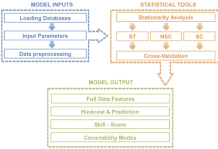
Figure 1.Schematic diagram illustrating the structure of the model.
Each permuted time series is used to repeat the calculation and compare the obtained results with the real values. Once this is done, the values obtained with the N permutations are taken to create a random distribution to finally determine the position of the real value within the distribution, which will indicate the statistical significance of the obtained value. This method has been described and used in previous research (Livezey and Chen, 1983; Barnett, 1995; Maia et al., 2007). The user inputs the level of statistical significance at which the test is applied, being the most used 90 % (0.10), 95 % (0.05) and 99 % (0.01).
3 S4CAST model
S4CAST v2.0 model is conceived as a statistical tool to study the predictability and teleconnections of variables that strongly co-vary with SSTA variability in remote and nearby locations to a particular region of study. The code has been developed as a MATLAB® toolbox. The software require-ments are variable and depend on user needs. The spatial resolution and size of data files used as inputs are directly proportional to memory requirements. The software gener-ates an “out of memory” message whenever it requests a segment of memory from the operating system that is larger than what is currently available. The model software consists of three main modules (Fig. 1), each composed of a set of sub-modules whose operation is described below.
3.1 Model Inputs
S4CAST v2.0 has a direct execution mode. By simply typing “S4cast” in the command window, the user is prompted to enter a series of input parameters in a simple and intuitive way.
3.1.1 Loading databases
The model is ready to work with Network Common Data Form (NetCDF) data files. There are different conventions to set the attributes of the variables contained in NetCDF files. In this way, the data structure must conform as far as possi-ble to the Cooperative Ocean/Atmosphere Research Service (COARDS) convention. Execution errors that may occur due to the selection of data files are easily corrected by minor modifications of data assimilation scripts. Data files can be easily introduced at the request of the user. Once downloaded from the website of a determined center of climate and envi-ronmental research, the user inserts data files into the direc-tory set by default (S4CAST_v2.0/data_files).
3.1.2 Input parameters
In order to correctly introduce the input parameters, it is con-venient to present some terms commonly used in seasonal forecasting. In this way, the forecast period corresponds to then-month seasonal period concerning the predictand for
which the forecast and hindcasts are performed. Moreover, the lead time refers to time expressed in months between the last month comprising the predictor monthly period and the first month comprising the forecast period. Thus, a medium-range forecast refers to a lead-time set to zero, while a long-range forecast refers to a lead-time equal or larger than 1 month. Strictly, we cannot speak about lead-time when the predictor monthly period partially or totally overlaps the forecast period. In this case we refer to lag-time expressed in moths between the last month comprising the forecast pe-riod and the last month for predictor pepe-riod. The relationship between lead-time and lag-time depends on the number of months comprising the forecast period. Finally, the forecast time is commonly used to describe the time gap expressed in months between the predictor and predictand monthly peri-ods, assuming the same concept represented by the lead time. In the first step, predictand and predictor data files are se-lected. In this way, the predictand field can be precipitation, SST, or any variable susceptible to be predicted from SSTA. The predictor is restricted to SST.
Once predictor and predictand fields are selected, the available common time period between them is analyzed and displayed so that the user is prompted to select the whole common period for analysis or other within it. The same temporal dimension in both fields is required in the statis-tical analysis to construct the cross-covariance matrix (see Sect. 2.1).
The next step is for selecting then-month forecast period
in which the predictand is considered. The model allows for a selection from 1 (n=1) to 4 (n=4) months. From the fore-cast period, the user determines a specific lead time, rela-tive to the predictor, from which medium range (lead time 0) or long range (lead time>0) forecast can be performed.
temporal overlapping between the forecast period and the predictor is also available by defining the monthly lags be-tween both fields from monthly lag 0 (synchronous) referred to the case in which the predictor and the predictand fields are taken at the same n-month period, through partial
overlap-ping to eliminate the overlapoverlap-ping (medium-range forecast). Note that synchronous and partially overlapping seasons be-tween predictor and predictand fields are not useful when re-ferring to predictability, although this option is available in order to perform simulations focused on the study of physi-cal mechanisms (teleconnections) between the predictor and predictand fields. Thus, it is worth noting that the model may be focused in the study of the predictability but it can be also used to detect teleconnections between SST (predictor) and a predictand field.
Monthly lags indicating forecast times (lead times) are user selectable. To illustrate the above, taking a hypothet-ical case in which the forecast period corresponds to the months of February–March–April (FMA) whatever the re-gion, the synchronous option will consider the predictor in FMA, while partially overlapping occurs when the predictor is taken for January–February–March (JFM) and December– January–February (DJF). Avoiding overlapping, lead time 0 will be NDJ (November–December–January), lead time 1 will be OND (October–November–December), lead time 2 will be SON (September–October–November), etc., with-out overlapping the FMA season of the previous year. Thus, the user can select any 3-month isolated period from FMA (synchronous) to MJJ (May–June–July).
Next, the spatial domains of both predictor and predictand fields are easily selected from its latitudinal and longitudinal values. Considering the above options, the user can select a sequence of successive monthly lags or only one so that the predictor is taken for the total amount of selected information (e.g., NDJ+OND+SON).
Later, there is the possibility of applying a filter to the time series of predictor and predictand fields. The current version uses a Butterworth filter, either as high-pass or low-pass fil-ter frequently used in climate-related studies (e.g., Roe and Steig, 2004; Enfield and Cid-Serrano, 2006; Mokhov and Smirnov, 2006; Ault and George, 2012; Schurer et al., 2013), although the selection of low-pass filter is not suitable for seasonal forecast and subsequently is not useful in the current version. Anyway, the possibility of selecting a low-pass filter is maintained in order to include decadal predictability in a future version of the model. The application of a filter allows the user to isolate the frequencies at which the variability op-erates, which can have different sources of predictability. In this way, the user selects the cutoff frequency, following the expression 2dt /T, being dt the sampling interval andT the
period to be filtered both in the same units of time. If no filter is applied, the raw data are used. There are plenty of filters that could be applied and future versions of the model will include different possibilities.
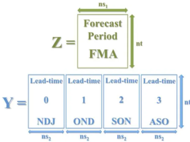
Figure 2. Predictand (Z) and predictor (Y) fields represented by their corresponding data matrices. The illustration relates to an example in which the forecast period covers the months February–March–April (FMA) and the predictor is selected for four distinct seasons: August–September–October (ASO, lead time=3); September–October–November (SON, lead time=2); October–November–December (OND, lead time=1); November– December–January (NDJ, lead time=0). Each of these sub-matrices for the predictor has the same temporal dimension (nt) and spatial dimension (ns2). The predictand may have a different spa-tial dimension (ns1)but the same temporal dimension (nt) to enable matrix calculations required by MCA methodology.
In the case of multiple time selection for predictor, the sta-tistical methodology is first applied considering the largest lead time and successively adding information for other lead times up to the present. Therefore, continuing with the ex-ample above in which the forecast period corresponds to FMA if selected lead times are from 0 to 3, the first pre-dictor selection is made considering the 3-months lead-time period (SON). After, the 2-months lead-time period is added (ASO+SON), next up to the period of 1-month delayed (ASO+SON+OND) and finally the case up to the period with a lead time equal to zero (ASO+SON+OND+NDJ). Previous example is illustrated in Fig. 2.
Once the matrices are determined for each predictor time selection, the statistical methodology is applied. Up to now, the model applies the MCA discriminant analysis technique, although other statistical methodologies will be included in future releases, including CCA or nonlinear methods as neu-ral network and Bayesian methodologies. As indicated in the previous section, MCA determines a new vector base in which the relations between the variables are maximized. Thus, it is important to choose a number of modes (principal directions) to be considered in the computations, selecting ei-ther a single mode or a set of them, always consecutive. The analysis of stationarity is performed for a single mode selec-tion. For multi-mode selection, the whole time series will be considered.
runs for the entire period and for those periods for which the relationships are considered stationary within it. This is in-ternally established by applying the method explained later in the Sect. 3.2.1.
3.1.3 Data preprocessing
From selected data files and input parameters previously de-fined, preprocessing of data is performed so that the data are prepared for implementing statistical methodology.
3.2 Statistical tools
At this point the statistical procedure described in the methodology is applied considering different periods based on the previously described stationary analysis.
3.2.1 Analysis of stationarity
Stationarity refers to changes along time in the co-variability pattern between two variables. Thus, we speak about sta-tionarity when such a pattern of co-variability keeps invari-ant within a time period and therefore will be non-stationary when showing changes. To evaluate how much the predictor (Y ) and the predictand (Z)fields are related to each other,
the model calculates running mean correlations between the expansion coefficients indicated in Eqs. (4) and (5) for the selectedkth mode along the record. This technique has been
widely used to determine the stationarity of the relationships between the time series of climate indices (e.g., Camberlin et al., 2001; Rimbu et al., 2003; Van Oldenborgh and Burg-ers, 2005). Next, the significance level of correlation coef-ficients is calculated according to the method explained in Sect. 2.2. In this way, stationary relationships between the predictor (Y) and the predictand (Z) fields are established
by applying a 21-year moving correlation window analysis between the leading expansion coefficients of both fields ob-tained from the discriminant analysis method (Sect. 2.1) us-ing the whole record in accordance with the evolution of the correlation coefficient. To do this, three types of 21-year moving correlation windows are user selectable: “delayed” to correlate 1 year and the 20 previous years; “centered” to correlate 1 year, the 10 previous years and the 10 next years; or “advanced” to correlate 1 year and the 20 next years. Note that delayed correlation coefficients are the most suitable in a forecast context when referring to future prediction. Nev-ertheless, centered and advanced correlation coefficients are also available for application no matter the aim of the user.
From previous analysis, three different periods are ana-lyzed depending on the stationarity of the predictability: use the significant correlation period (hereinafter SC) for which the expansion coefficients are significantly correlated, use no significant correlation period (hereinafter NSC) and work with the entire period (hereinafter EP). The model performs all calculations for each period separately and, from them,
the simulated maps (hindcasts) of the predictand for each year are calculated by applying cross-validation.
3.2.2 Model validation
Cross-validation is used in climate forecasting as part of sta-tistical models when assessing forecast skill (Michaelsen, 1987; Barnston and Van den Dool, 1993; Elsner and Schmertmann, 1994). This method is intended as a model validation technique in which the data for the predictor and the predictand for a given time step is removed from the anal-ysis to make an estimate of it with the rest of data, compar-ing the simulated value with the removed one. In this way, a cross-validated hindcast is obtained. In the S4CAST model, the leave-one-out method is applied as described by Dayan et al. (2014). From the comparison between the predicted value and the original one, the skill of the model can be inferred us-ing different skill scores. S4CAST considers the Pearson cor-relation coefficients and the root mean square error (RMSE) although other scores will be introduced in future versions. 3.3 Model outputs
Modes of co-variability are related to spatial patterns of dif-ferent variables that co-vary over time, and thus are linked to each other. In the case of MCA, the covariance matrix is computed and the SVD method is applied to provide a new basis of eigenvectors for the predictor and predictand fields which covariance is maximized. The obtained singu-lar vectors describe spatial patterns of anomalies in each of the variables that tend to be related to each other. Regres-sion and correlation maps and corresponding expanRegres-sion co-efficients determine each mode of co-variability for the pre-dictor and predictand fields. The expansion coefficients indi-cate the weight of these patterns in each of the time steps. Thus, regression and correlation co-variability maps can be represented. This is done with the original anomalous matrix, highlighting those grid points whose time series are highly correlated with the obtained expansion coefficients, showing large co-variability and determining the key regions of pre-diction. To represent it, regression and correlation maps are calculated to analyze the coupling between variables and to understand the physical mechanisms involved in the link.
On the other hand, the time series of the expansion coeffi-cients determine the scores of the regression and correlation maps at each time along the study period. The model repre-sents the expansion coefficients used to calculate the regres-sion coefficients. Thus, those years in which the expanregres-sion coefficients for the predictor and the predictand are highly correlated will coincide with years in which we can expect a better estimation.
obtaining correlation and RMSE maps and time series. On the one hand, maps are obtained calculating for each grid point the skill scores between the hindcast and the observed maps. On the other hand, time series are obtained for each time by applying correlation and RMSE between the area average of the observed and estimated maps. Some com-ments on these techniques are addressed by Barnston (1992). The S4CAST model generates the hindcast within the EP, SC and NSC periods separately from applying the one-leave-out method (Dayan et al., 2014) and then the statistical method-ology.
4 Application of the model: case studies
Two different case studies have been simulated as benchmark examples. Both cases are focused on the predictive ability of the tropical Atlantic SSTA. In a first simulation, the pre-dictand field corresponds to Sahelian rainfall. In a second simulation, winter tropical Pacific SSTA have been used as predictand field. The links between tropical Atlantic Ocean and the two variables selected as predictand fields have been widely studied exhibiting non-stationary relationships. The results obtained by applying the model have been contrasted in the following sections. Tables 1 and 2 list the entries for both case studies to be easily reproduced by the user. 4.1 Tropical Atlantic – Sahelian rainfall
In this first case study the model has been applied to val-idate its use in the study of seasonal rainfall predictability in the Sahel taking tropical Atlantic as predictor field. The West African Monsoon (WAM) is characterized by a strong seasonal rainfall regime that occurs from July to September related to the semi-annual shift of the Intertropical Conver-gence Zone (ITCZ) together with the presence of a strong thermal gradient between the Sahara and the ocean in the Gulf of Guinea. The interannual fluctuations in seasonal rain-fall are due to various causes; the changes in global SST are the main driver of WAM variability (Folland, 1986; Palmer, 1986; Fontaine et al., 1998; Rodríguez-Fonseca et al., 2015). Particularly, several observational studies suggest the influ-ence of tropical Atlantic SSTA on the WAM at interannual timescales (Giannini et al., 2003; Polo et al., 2008; Joly and Voldoire, 2009; Nnamchi and Li, 2011).
Regarding the input parameters (Table 1), the predic-tand field corresponds to precipitation from GPCC Full Data Reanalysis monthly means of precipitation appended with GPCC monitoring data set from 2011 onwards with a resolution of 1.0◦×1.0◦ covering the period from
Jan-uary 1901 to March 2015 (Rudolf et al., 2010; Becker et al., 2013; Schneider et al., 2014; http://gpcc.dwd.de). The fore-cast period consists of July–August–September (JAS), com-puting seasonal anomalous rainfall in the Sahelian domain (18◦W–10◦E; 12–18◦N). No frequency filter is applied for
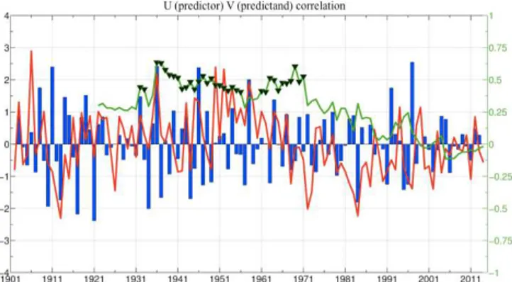
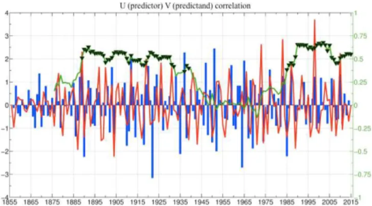
Figure 3.Shown are 21-year moving correlation windows (green line) between the expansion coefficientsU corresponding to trop-ical Atlantic SSTA (predictor, blue bars) andV corresponding to Sahelian anomalous rainfall (predictand, red line) obtained for the leading mode of co-variability from MCA analysis. Shaded trian-gles indicate significant correlation under a Monte Carlo Test at 90 %.
predictand. The predictor field corresponds to NOAA Ex-tended Reconstructed SST (ERSST) V3b monthly means of SST with a resolution of 2.0◦×2.0◦ spanning the
pe-riod from January 1854 to May 2015 (Smith and Reynolds, 2003, 2004; Smith et al., 2008; http://www.esrl.noaa.gov/ psd/data/gridded/data.noaa.ersst.html). The spatial domain corresponds to southern subtropical and equatorial Atlantic band (60◦W–20◦E; 20◦S–4◦N). A high-pass filter with
cut-off frequency set to 7 years has been applied to the predictor time series in order to analyze the influence of SSTA inter-annual variability, which includes leading oceanic interan-nual variability modes such as the Atlantic equatorial mode (AEM) (Polo et al., 2008) or the South Atlantic Ocean dipole (SAOD) (Nnamchi et al., 2011). Medium-range forecast has been taken into account setting the lead time to zero (equiv-alent to monthly lag 3). In this way, April–May–June (AMJ) is the selected season for predictor.
For applying the methodology, the leading mode of co-variability (k=1) has been selected. The correlation curve (Fig. 3) reflects the stationary periods (SC and NSC) within EP period as stated in Sect. 3.2.1. The SC period is almost restricted to years from 1932 to 1971 with some exceptions. The remaining years are taken to analyze the predictability for the NSC period.
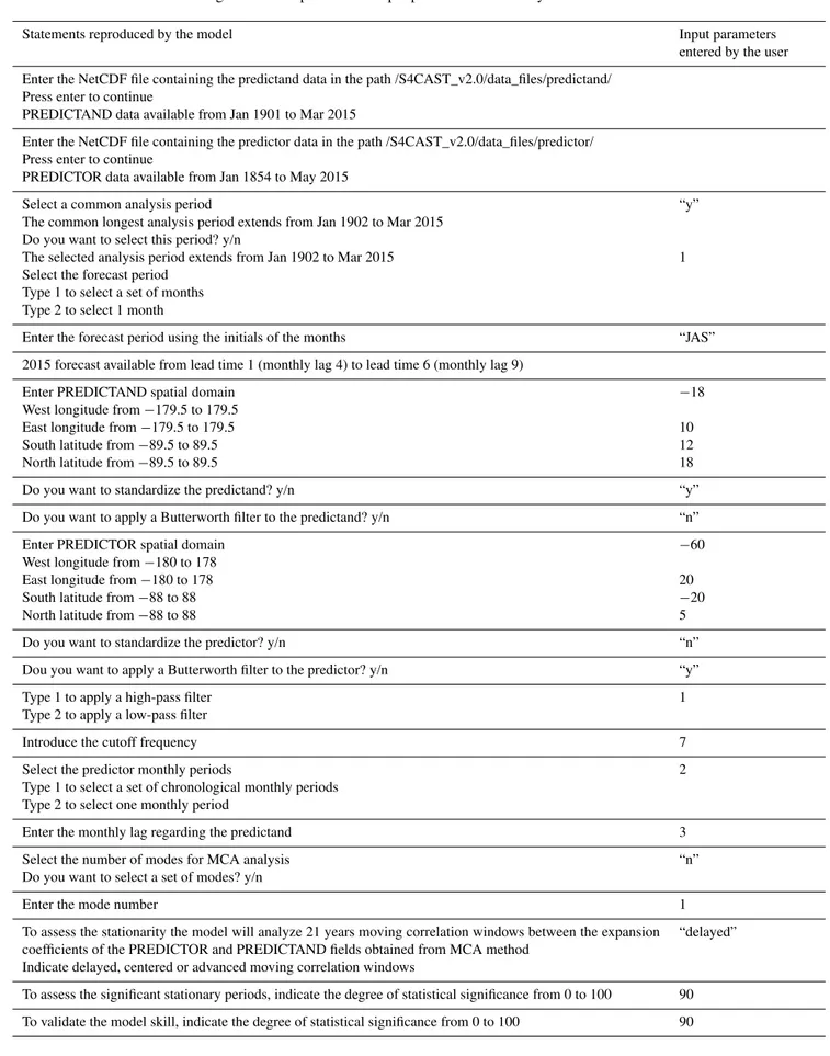
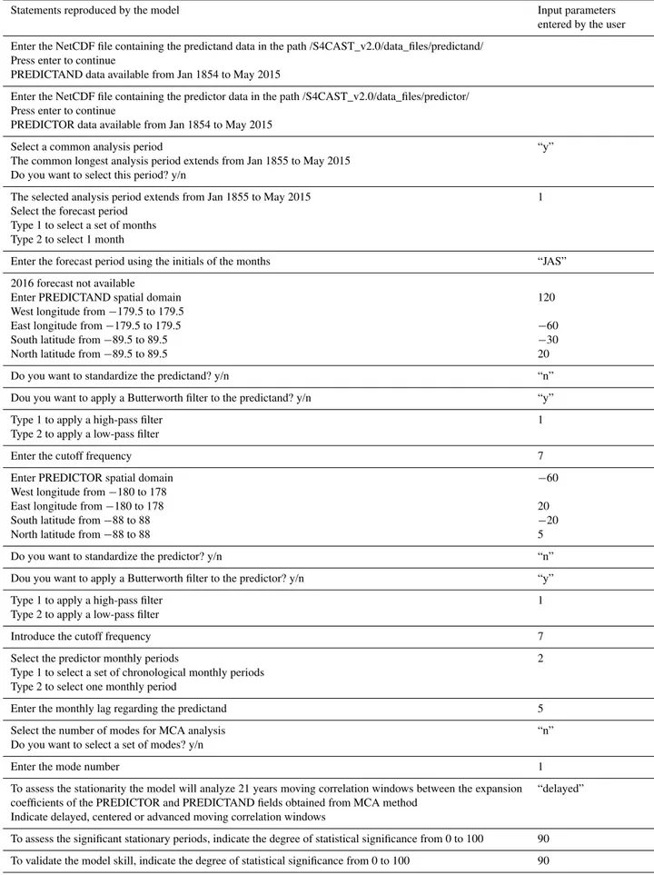
Table 1.Input parameters used to reproduce the first case study. Left column represents the statements reproduced by the model with the same format as in the simulation. Right column represents the input parameters entered by the user.
Statements reproduced by the model Input parameters
entered by the user
Enter the NetCDF file containing the predictand data in the path /S4CAST_v2.0/data_files/predictand/ Press enter to continue
PREDICTAND data available from Jan 1901 to Mar 2015
Enter the NetCDF file containing the predictor data in the path /S4CAST_v2.0/data_files/predictor/ Press enter to continue
PREDICTOR data available from Jan 1854 to May 2015
Select a common analysis period
The common longest analysis period extends from Jan 1902 to Mar 2015 Do you want to select this period? y/n
“y”
The selected analysis period extends from Jan 1902 to Mar 2015 Select the forecast period
Type 1 to select a set of months Type 2 to select 1 month
1
Enter the forecast period using the initials of the months “JAS”
2015 forecast available from lead time 1 (monthly lag 4) to lead time 6 (monthly lag 9)
Enter PREDICTAND spatial domain
West longitude from−179.5 to 179.5
−18
East longitude from−179.5 to 179.5 10
South latitude from−89.5 to 89.5 12
North latitude from−89.5 to 89.5 18
Do you want to standardize the predictand? y/n “y”
Do you want to apply a Butterworth filter to the predictand? y/n “n”
Enter PREDICTOR spatial domain
West longitude from−180 to 178
−60
East longitude from−180 to 178 20
South latitude from−88 to 88 −20
North latitude from−88 to 88 5
Do you want to standardize the predictor? y/n “n”
Dou you want to apply a Butterworth filter to the predictor? y/n “y”
Type 1 to apply a high-pass filter Type 2 to apply a low-pass filter
1
Introduce the cutoff frequency 7
Select the predictor monthly periods
Type 1 to select a set of chronological monthly periods Type 2 to select one monthly period
2
Enter the monthly lag regarding the predictand 3
Select the number of modes for MCA analysis Do you want to select a set of modes? y/n
“n”
Enter the mode number 1
To assess the stationarity the model will analyze 21 years moving correlation windows between the expansion coefficients of the PREDICTOR and PREDICTAND fields obtained from MCA method
Indicate delayed, centered or advanced moving correlation windows
“delayed”
To assess the significant stationary periods, indicate the degree of statistical significance from 0 to 100 90
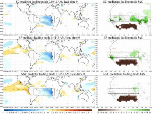
Figure 4.Regression maps obtained for the leading mode by applying MCA between SSTA in the tropical Atlantic (predictor) and western Sahel rainfall (predictand). Left column represents the homogeneous regression map done by projecting the expansion coefficientUonto global SSTA (◦C). Right column represents the heterogeneous regression map done by projecting expansion coefficientUonto the anomalous Sahelian rainfall (mm day−1). Period SC (top panels), EP (middle panels) and NSC (bottom panels). Rectangles show the selected regions for predictor and predictand fields considered in the MCA analysis. Values are plotted in regions where statistical significance under a Monte Carlo test is higher than 90 %.
the tropical Atlantic SST as a dominant factor in the WAM variability at interannual and seasonal timescales (Janowiak, 1988; Janicot, 1992; Fontaine and Janicot, 1996). Losada et al. (2010b) found how the response to an isolated positive equatorial Atlantic Niño event is a dipolar rainfall pattern in which the decrease of rainfall in Sahel is related to the in-crease of rainfall in Guinea (as in Fig. 4) due to changes in the sea–land pressure gradient between Gulf of Guinea SSTs and the Sahel. Mohino et al. (2011) and Rodríguez-Fonseca et al. (2011) have found in the observations how this dipolar behavior takes place for some particular decades coinciding with the SC periods, confirming in this way the correct determination of the leading co-variability mode by the model. When considering the EP period (Fig. 4, middle panels), a co-variability pattern similar to that observed for the SC period is appreciated with small differences. Regard-ing the predictand field, the anomalous rainfall signal is less intense when compared to SC. For the predictor, the cool-ing in the tropical Atlantic is accompanied by opposite weak anomalies in the north subtropical and tropical Pacific. Re-garding the NSC period (Fig. 4, bottom panels), as for the previous periods (SC, EP) a cooling in the tropical Atlantic is observed concerning the predictor associated with negative rainfall anomalies in the Gulf of Guinea and a weak positive signal in the eastern Sahel, virtually disappearing the rainfall
dipole. The global SSTA regression map shows a significant warming in the tropical Pacific. The opposite pattern should be considered under negative scores of the expansion coeffi-cient.
The results presented above support the existence of a non-stationary behavior of the teleconnections between SSTA variability and rainfall associated with WAM. Several au-thors have addressed the dipolar anomalous rainfall pattern as a response of an isolated tropical Atlantic warming (cool-ing) (Rodríguez-Fonseca et al., 2011; Losada et al., 2010a, b; Mohino et al., 2011) restricted to the period 1957–1978 in the observations. The uniform rainfall signal over the whole of West Africa, with negative anomalies related to a cool-ing over the tropical Atlantic and an opposite sign pattern over the tropical Pacific, is only observed for the period from 1979 in advance. These results agree with Losada et al. (2012), who focused on non-stationary influences of trop-ical global SST in WAM variability, explaining how the dis-appearance of the dipole was due to the counteracting effect of the anomalous responses of the Pacific and Atlantic on the Sahel. Recently, Diatta and Fink (2014) have documented similar non-stationary relationships.
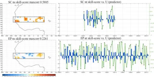
ob-Figure 5.Skill-score validation using Pearson correlation coefficients between observations and hindcasts. Left column corresponds to the spatial validation for each point in space. Right column corresponds to validation time series (green line) between hindcasts and observations considering only the regions indicated by positive significant spatial correlation. Period SC (top panels) and EP (bottom panels). Significant correlation values for time series are indicated by shaded triangles. Blue bars correspond to the expansion coefficient (U) of the SSTA (predictor). Significant values are plotted from a 90 % statistical significance under a Monte Carlo test.
served when considering the SC periods instead of the whole period (EP). This result points to a better spatial distribution of the significant values for particular decades in which the signal extends to a larger spatial domain. In order to analyze the performance of the simulation for each particular year, the correlation between observed and predicted maps at each time step is calculated and shown in Fig. 5. There is no skill when NSC period is considered (Fig. 6). Since it has only been considered the leading mode of co-variability, the time series of validation between observed and simulated rainfall should evolve following the absolute values of the expansion coefficients. Thus, when the expansion coefficient (U) of the
predictor (SST) shows high scores in the leading mode, good hindcasts are obtained.
4.2 Tropical Atlantic – tropical Pacific
A non-stationary behavior in the association between tropi-cal Atlantic and tropitropi-cal Pacific SSTA has been recently doc-umented in some research suggesting that the tropical At-lantic SSTA during the boreal summer could be a potential predictor of winter tropical Pacific SSTA variability after the 1970s (Rodríguez-Fonseca et al., 2009; Ding et al., 2012). In this section, the S4CAST model has been applied to corrobo-rate the non-stationarity in the teleconnection between tropi-cal Atlantic considered as predictor field and tropitropi-cal Pacific variability, a feature that has been also demonstrated in Mar-tin del Rey et al. (2015).
The input parameters are listed in Table 2. Both predictor and predictand fields corresponds to NOAA ERSST intro-duced in the previous section (Sect. 4.1), covering the period from January 1854 to May 2015. The forecast period con-sists of December–January–February–March (DJFM). The
Figure 6.Skill-score validation using Pearson correlation coeffi-cients between observations and hindcasts for each point in space corresponding to NSC period. Significant values are plotted from a 90 % statistical significance under a Monte Carlo test.
selected region for predictand corresponds to SSTA in the tropical Pacific domain (120◦E–60◦W; 30◦S–20◦N), while
the predictor corresponds to tropical Atlantic SSTA (60◦W–
20◦E; 20◦S–4◦N) and has been considered for the
Table 2.Input parameters used to reproduce the second case study. Left column represents the statements reproduced by the model. Right column represents the input parameters.
Statements reproduced by the model Input parameters
entered by the user
Enter the NetCDF file containing the predictand data in the path /S4CAST_v2.0/data_files/predictand/ Press enter to continue
PREDICTAND data available from Jan 1854 to May 2015
Enter the NetCDF file containing the predictor data in the path /S4CAST_v2.0/data_files/predictor/ Press enter to continue
PREDICTOR data available from Jan 1854 to May 2015 Select a common analysis period
The common longest analysis period extends from Jan 1855 to May 2015 Do you want to select this period? y/n
“y”
The selected analysis period extends from Jan 1855 to May 2015 Select the forecast period
Type 1 to select a set of months Type 2 to select 1 month
1
Enter the forecast period using the initials of the months “JAS”
2016 forecast not available Enter PREDICTAND spatial domain
West longitude from−179.5 to 179.5
120
East longitude from−179.5 to 179.5 −60
South latitude from−89.5 to 89.5 −30
North latitude from−89.5 to 89.5 20
Do you want to standardize the predictand? y/n “n”
Dou you want to apply a Butterworth filter to the predictand? y/n “y”
Type 1 to apply a high-pass filter Type 2 to apply a low-pass filter
1
Enter the cutoff frequency 7
Enter PREDICTOR spatial domain
West longitude from−180 to 178
−60
East longitude from−180 to 178 20
South latitude from−88 to 88 −20
North latitude from−88 to 88 5
Do you want to standardize the predictor? y/n “n”
Dou you want to apply a Butterworth filter to the predictor? y/n “y”
Type 1 to apply a high-pass filter Type 2 to apply a low-pass filter
1
Introduce the cutoff frequency 7
Select the predictor monthly periods
Type 1 to select a set of chronological monthly periods Type 2 to select one monthly period
2
Enter the monthly lag regarding the predictand 5
Select the number of modes for MCA analysis Do you want to select a set of modes? y/n
“n”
Enter the mode number 1
To assess the stationarity the model will analyze 21 years moving correlation windows between the expansion coefficients of the PREDICTOR and PREDICTAND fields obtained from MCA method
Indicate delayed, centered or advanced moving correlation windows
“delayed”
To assess the significant stationary periods, indicate the degree of statistical significance from 0 to 100 90
Figure 7.Shown are 21-year moving correlation windows (green line) between the expansion coefficientsU corresponding to trop-ical Atlantic SSTA (predictor, blue bars) andV corresponding to tropical Pacific SSTA (predictand, red line) obtained for the leading mode of co-variability from MCA analysis between predictor and predictand fields. Shaded triangles indicate significant correlation under a Monte Carlo Test at 90 %.
The correlation curve (Fig. 7) presents the SC period clearly divided into two intervals: from 1889 to 1939 and from 1985 up to the present (2015). Consequently, the NSC period corresponds to the remaining years within the study period (1854–2015).
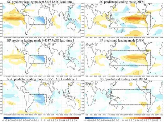
The leading mode (Fig. 8) for the periods SC, NSC and EP explains 52, 28 and 43 % of co-variability, respectively. Regarding the SC (Fig. 8; top panels) and EP (Fig. 8; middle panels) periods, it is observed how a cooling (warming) in the tropical Atlantic is related to a warming (cooling). Thus, the co-variability pattern is defined by opposite sign anomalies between predictor and predictand fields, although the mag-nitude of the anomalies is greater concerning the SC period. Considering the NSC period (Fig. 8; bottom panels), a signal in tropical Pacific is not observed in response to the tropical Atlantic cooling (warming).
Previous results are in agreement with former studies in which a similar tropical SSTA pattern with opposite tem-perature anomalies in the equatorial Atlantic and Pacific in summer has been documented to occur in the decades within the SC period (Rodríguez-Fonseca et al., 2009; Martin-Rey et al., 2012). Thus, Martín-Rey et al. (2014, 2015) point to a non-stationary relationship that seems to take place in the early 20th century and after the 1970s, confirming the cor-rect determination of the leading co-variability mode by the model.
The mechanism, from which the teleconnection takes place, has been explained by Polo et al. (2015), who sug-gest that a cooling in the equatorial Atlantic results in en-hanced equatorial convection, altering the Walker circulation and consequently enhancing subsidence and surface wind di-vergence over the equatorial Pacific during the period JASO. The anomalous wind piles up water in the western tropical Pacific, triggering a Kelvin wave eastward from autumn to winter, setting up the conditions for a cold event in the
equa-torial east Pacific during the period DJFM. Considering a cooling in the tropical Atlantic, the opposite sequence takes place.
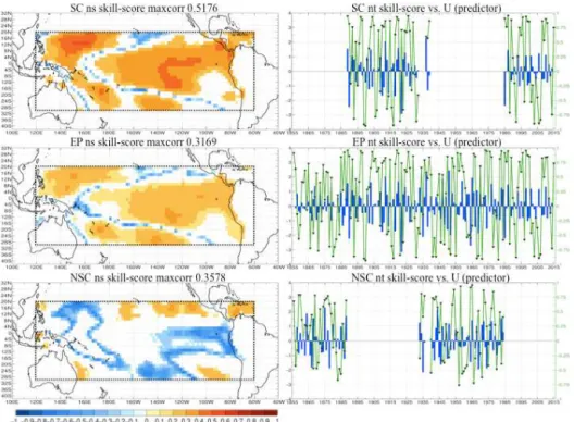
The skill of the model in reproducing tropical Pacific SSTA (Fig. 9) is also restricted to stationary conditions. Thus, depending on the considered sequence of decades within the period EP (Fig. 9; middle panels), the model pro-vides better results for period SC (Fig. 9; top panels), while it is not able to produce reliable estimations when period NSC (Fig. 9; bottom panels) is taken into account. These results highlight the need to consider different periods and possible modulations when tackling seasonal predictability of tropical Pacific SSTA, in agreement with recent results of Martin del Rey et al. (2015).
5 Discussion and conclusions
It is well known how dynamical models need to be to pro-duce very accurate seasonal climate forecast for non-ENSO events, partly due to the presence of strong biases in some re-gions, such as the tropical Atlantic (Barnston et al., 2015). In contrast, statistical models, despite being a useful and effec-tive supplement, are mostly unable to reproduce the nonlin-earity in the ocean–atmosphere system, exceptions include neural networks and Bayesian methods. Attempts to imple-ment new statistical models constitute a fundaimple-mental con-tribution aimed to enhance and complement the dynamical models. Nevertheless, statistical models have evolved linked to dynamical models, either as an alternative or within them as a hybrid model.
Following this reasoning, this paper introduces the S4CAST v2.0 model. The model was created from the first version (S4CAST v1.0) developed as the main part of a co-operation project between theLaboratoire de Physique de l’Atmosphère et de l’Océan Siméon Fongangof the Univer-sity Cheik Anta Diop (UCAD) in Dakar (Senegal) and the ComplutenseUniversity of Madrid (UCM) within the VIII UCM Call for Cooperation and Development projects (VR: 101/11) and was named “Creation and Donation of a sta-tistical seasonal forecast model for West African rainfall”. Thereby, the authors wanted to respect the number of the do-nation version despite not having a publication. As a brief explanation on the history, the original model was restricted to study the predictability of West African rainfall from trop-ical global SSTA using much more limited input parameters that those described in this work for version 2.0. Thus, the reason for developing and improve the model for publication is the motivation arising from colleagues in different institu-tions along Africa and Europe to expand the model and use it as an alternative tool to look for SST-related predictability due to the strong SST bias that coupled dynamical models exhibit nowadays.
Figure 8.Regression maps obtained for the leading mode by applying MCA between SSTA in the tropical Atlantic (predictor) and SSTA in the tropical Pacific (predictand). Left column represents the homogeneous regression map done by projecting the expansion coefficient U onto global SSTA (◦C) for predictor seasonal period. Right column represents the heterogeneous regression map done by projecting expansion coefficientUonto global SSTA (◦C) for predictand seasonal period. Period SC (top panels), EP (middle panels) and NSC (bottom panels). Rectangles show the selected regions for predictor and predictand fields considered in the MCA analysis. Values are plotted in regions where statistical significance under a Monte Carlo test is higher than 90 %.
any climate-related variable susceptible of being predicted from it, the concept of stationarity is raised as one of the motivating factors in creating the S4CAST model. The sta-tionarity refers to changes in the co-variability patterns be-tween the predictor and the predictand fields along a given sequence of decades, so that it can be kept invariant (station-ary) or changing (non-station(station-ary). This concept has been ad-dressed by different authors (Janicot et al., 1996; Fontaine et al., 1998; Rodríguez-Fonseca et al., 2009, 2011; Mohino et al., 2011; Martín-Rey et al., 2012; Losada et al., 2012) and becomes the main novelty and contribution introduced by S4CAST as a key factor to consider in seasonal forecast-ing provided by current prediction models, either dynami-cal or statistidynami-cal. Thus, S4CAST model is an alternative to enhance and complement the estimates made by dynamical models, which have a number of systematic errors to ade-quately reproduce the tropical climate variability (Biasutti et al., 2006; Richter and Xie, 2008; Wahl et al., 2011; Doi et al., 2012; Richter et al., 2012; Bellenger et al., 2013; Brown et al., 2013; Li and Xie, 2013; Toniazzo and Woolnough, 2013; Vannière et al., 2013; Xue et al., 2013). For the time being, the S4CAST model cannot be applied for strict operational forecasts, although its application in determining stationary relationships between two fields and their co-variability
pat-terns can be crucial for improving the estimates provided by the operating prediction models currently used.
The model is proposed for use in two areas: the study of seasonal predictability and the study of teleconnections, both based on the influence of SST. On the one hand, we refer to predictability when predictor is considered from a lead time equal to 0 months (medium-range forecast) in advance (long-range forecast). On the other hand, we speak about the study of teleconnections when predictor seasonal selection partially or totally overlaps (synchronous) the forecast pe-riod, meaning that one cannot speak about lead time, instead we speak about a monthly lag between the last month in the forecast period and the last month comprising the predictor monthly period.
Figure 9.Skill-score validation using Pearson correlation coefficients between observations and hindcasts. Left column corresponds to the spatial validation for each point in space. Right column corresponds to validation time series (green line) between hindcasts and observations considering only the regions indicated by positive significant spatial correlation. Period SC (top panels), EP (middle panels), and NSC (bottom panels). Significant correlation values for time series are indicated by shaded triangles. Blue bars correspond to the expansion coefficient (U) of the SSTA (predictor). Significant values are plotted from a 90 % statistical significance under a Monte Carlo test.
June 2015. Thus, the model constructs the regression coeffi-cient by using the common period until November 2014. Re-gression coefficients along with predictor data (AMJ 2015) will provide the forecast for SON 2015. In this way, the model first checks data availability related to the input pa-rameters and shows by screen if future forecast is enabled. If enabled, the model performs three types of forecast by com-puting the regression coefficient for each period (SC, NSC, EP). Finally, the user should determine the better forecast by a study of the modulations of each stationary period and the sequence of hindcasts immediately preceding the present.
In the applications shown in this paper, we have focused in the results from MCA. This statistical methodology, along with canonical correlation analysis (CCA), have been widely used on studies of predictability during the last decades (Barnston and Ropelewski, 1992; Bretherton et al., 1992; Wallace et al., 1992; Barnston and Smith, 1996; Fontaine et al., 1999; Korecha and Barnston, 2007; Barnston and Tip-pet, 2014; Recalde-Coronel et al., 2014). Integration of the methodology and intuitive use through a user interface are some of the main advantages of the S4CAST model, allow-ing the selection of a big number of inputs. Future releases of the model will include other methodologies that are currently being introduced and tested.
Originally, the model was created to tackle the study of the predictability of anomalous rainfall associated with WAM,
which co-varies in a different way with the tropical band of Atlantic and Pacific ocean basins, being an indicator of non-stationarity (Losada et al., 2012). The transition between SC and NSC periods, around the 1970s, has served as the starting point of many studies focusing on the influence of global SSTA before and after that period (Mohino et al., 2011; Rodríguez-Fonseca et al., 2011, 2015; Losada et al., 2012) while being one of the motivations to create S4CAST. The choice of the case study related to Sahelian rainfall predictability is motivated by the following reasons: on the one hand, SST in the tropical Atlantic is well known to strongly influence the dynamics of the ITCZ (Fontaine et al., 1998) which in turn determines the subsequent WAM. Nevertheless, dynamical models do not reproduce the in-fluence of SST on the ITCZ (Lin, 2007; Richter and Xie, 2008; Doi et al., 2012; Toniazzo and Woolnough, 2013) be-coming the statistical prediction an alternative way to pre-dict WAM variability. The second reason is related to the non-stationary influence of the tropical Atlantic on Sahelian rainfall reported in some studies (Janicot et al., 1996, 1998; Ward, 1998; Rodríguez-Fonseca et al., 2011; Mohino et al., 2011; Losada et al., 2012).
discov-ered relationship (Rodríguez-Fonseca et al., 2009; Ding et al., 2012; Polo et al., 2015) that has been found to be non-stationary (Martín del Rey et al., 2014, 2015).
The application of moving correlation windows between expansion coefficients obtained from MCA analysis results in three periods of stationarity depending on the statistically significant correlation: entire period (EP), significant correla-tion period (SC) and no-significant correlacorrela-tion period (NSC). For the case in which non-stationarity is considered, we re-fer to EP period, assuming changes in co-variability patterns. Stationarity is referred to SC and NSC periods. These peri-ods may slightly vary depending on the type of moving cor-relation windows: advanced, centered or delayed. Stationary analysis to determine the three different work periods (SC, NSC, EP) is limited to the selection of a single mode of co-variability. When selecting a set of modes, the stationarity analysis is not applied so that simulations are only developed for EP period, whereby the whole time series is considered for both the predictor and predictand fields.
Three conditions may enhance the degree of confidence in a given predictor. The first has to do with the selection of moving correlation windows (see Sect. 3.1.2) used to deter-mine the working scenarios (SC, NSC, EP). Delayed moving correlation windows can help in this task. Thus, if correla-tion coefficients between the expansion coefficients (U and V) exhibit significant values for the present year and the
pre-vious 21 study years, greater confidence is assumed for the predictor. The second condition is determined by the value of the expansion coefficient (U) for the current year so that
the higher its value, the better the forecast. The last condition has to do with the percentage of variance explained by the se-lected co-variability mode, the higher its value, the better the forecast. Nevertheless, despite previous conditions, the influ-ence of other remote and nearby oceanic predictors must be considered in order to provide a full and reliable predictabil-ity study.
So far, the data files used as predictor and predictand fields correspond to observations and reanalysis from sev-eral institutions. The use of new data files is simple and can be performed according to user needs. The upgrade of data files from respective websites must be checked periodically to strengthen the results. In addition, it is also advisable to launch the same simulations using different data files in or-der to compare the results and assess the robustness of the forecast. The results shown in this work for different selec-tions have been verified by following these criteria.
The results obtained by using the S4CAST model put forward the consideration of non-stationarity in the co-variability patterns and therefore in climatic teleconnections. Thus, it is important to determine the multidecadal modula-tor of the interannual variability in order to know which pre-dictor is the one affecting in particular periods and regions (Rodríguez-Fonseca et al., 2015).
Code availability
The model consists of a software package organized in fold-ers containing libraries, functions and scripts developed as a MATLAB® toolbox from version R2010b onwards. Two of the folders, named asmexcdfandnetcdf_toolbox, corre-sponds to libraries needed for working with NetCDF files and have been downloaded from www.mexcdf.sourceforge.net and built into the model. The file containing the model core with the executable code is named S4core. Once the tool-box has been added to the MATLAB® path and by sim-ply typing “S4cast” in the command window, the user is prompted to enter a number of input parameters required to launch a simulation. The software packageS4plot ded-icated to plot figures has been added so that the user can use this software by typing “figures” in the com-mand window. Note that figures presented in this work have been further improved manually. The code is open access and can be downloaded from the Zenodo reposi-tory (doi:10.5281/zenodo.15985) in the URL https://zenodo. org/record/15985. To facilitate the execution of the model leading to the results shown in this paper, used data files that have been previously defined in Sect. 4, are included in the directories /S4CAST_v2.0/data_files/predictand and /S4CAST_v2.0/data_files/predictor. The second case study requires NOAA ERSST as predictor and predictand. The code has been thoroughly analyzed by using several data files and input parameters. However, the emergence of software bugs is not ruled out, being mostly associated with problems to adapt and use NetCDF files. To solve these hypothetical code bugs, please do not hesitate to contact authors.
The Supplement related to this article is available online at doi:10.5194/gmd-8-3639-2015-supplement.
Acknowledgements. The research leading to these results received funding from the PREFACE-EU project (EU FP7/2007-2013) un-der grant agreement no. 603521, Spanish national project MINECO (CGL2012-38923-C02-01) and the VR: 101/11 project from the VIII UCM Call for Cooperation and Development projects. We also appreciate the work done by SOURCEFORGE.NET®staff in creating NetCDF libraries for MATLAB®, and of course, thanks also to the reviewers, editors and their advice and/or criticism.
References
Adams, R. M., Chen, C. C., McCarl, B. A., and Weiher, R. F.: The economic consequences of ENSO events for agriculture, Clim. Res., 13, 165–172, 1999.
Ault, T. R., Cole, J. E., and St George, S.: The amplitude of decadal to multidecadal variability in precipitation simulated by state-of-the-art climate models, Geophys. Res. Lett., 39, L21705, doi:10.1029/2012GL053424, 2012.
Baboo, S. S. and Shereef, I. K.: An efficient weather forecasting system using artificial neural network, International Journal of Environmental Science and Development, 1, 2010–0264, 2010. Barnett, T. P.: Monte Carlo climate forecasting, J. Climate, 8, 1005–
1022, 1995.
Barnett, T. P. and Preisendorfer, R.: Origins and levels of monthly and seasonal forecast skill for United States surface air tem-peratures determined by canonical correlation analysis, Mon. Weather Rev., 115, 1825–1850, 1987.
Barnett, T. P., Graham, N., Pazan, S., White, W., Latif, M., and Flügel, M.: ENSO and ENSO-related predictability. Part I: Pre-diction of equatorial Pacific sea surface temperature with a hy-brid coupled ocean-atmosphere model, J. Climate, 6, 1545–1566, 1993.
Barnston, A. G.: Correspondence among the correlation, RMSE, and Heidke forecast verification measures; refinement of the Hei-dke score, Weather Forecast., 7, 699–709, 1992.
Barnston, A. G. and Ropelewski, C. F.: Prediction of ENSO episodes using canonical correlation analysis, J. Climate, 5, 1316–1345, 1992.
Barnston, A. G. and Smith, T. M.: Specification and prediction of global surface temperature and precipitation from global SST us-ing CCA, J. Climate, 9, 2660–2697, 1996.
Barnston, A. G. and Tippett, M. K.: Climate information, outlooks, and understanding – where does the IRI stand?, Earth Perspec-tives, 1, 1–17, 2014.
Barnston, A. G. and van den Dool, H. M.: A degeneracy in cross-validated skill in regression-based forecasts, J. Climate, 6, 963– 977, 1993.
Barnston, A. G., van den Dool, H. M., Rodenhuis, D. R., Ro-pelewski, C. R., Kousky, V. E., O’Lenic, E. A., and Leetmaa, A.: Long-lead seasonal forecasts-Where do we stand?, B. Am. Meteorol. Soc., 75, 2097–2114, 1994.
Barnston, A. G., He, Y., and Glantz, M. H.: Predictive skill of statis-tical and dynamical climate models in SST forecasts during the 1997–98 El Niño episode and the 1998 La Niña onset, B. Am. Meteorol. Soc., 80, 217–243, 1999.
Barnston, A. G., Tippet, M. K., van den Dool, H. M., and Unger, D. A.: Toward an Improved Multi-model ENSO Prediction, J. Appl. Meteorol. Clim., 54, 1579–1595, doi:10.1175/JAMC-D-14-0188.1, 2015.
Becker, A., Finger, P., Meyer-Christoffer, A., Rudolf, B., Schamm, K., Schneider, U., and Ziese, M.: A description of the global land-surface precipitation data products of the Global Precipita-tion Climatology Centre with sample applicaPrecipita-tions including cen-tennial (trend) analysis from 1901–present, Earth Syst. Sci. Data, 5, 71–99, doi:10.5194/essd-5-71-2013, 2013.
Bellenger, H., Guilyardi, E., Leloup, J., Lengaigne, M., and Vialard, J.: ENSO representation in climate models: from CMIP3 to CMIP5, Clim. Dynam., 42, 1999–2018, 2013.
Biasutti, M., Sobel, A. H., and Kushnir, Y.: AGCM precipitation biases in the tropical Atlantic, J. Climate, 19, 935–958, 2006. Bjerknes, J.: Atmospheric teleconnections from the equatorial
pa-cific 1, Mon. Weather Rev., 97, 163–172, 1969.
Bretherton, C. S., Smith, C., and Wallace, J. M.: An intercompar-ison of methods for finding coupled patterns in climate data, J. Climate, 5, 541–560, 1992.
Brown, J. N., Gupta, A. S., Brown, J. R., Muir, L. C., Risbey, J. S., Whetton, P., and Wijffels, S. E.: Implications of CMIP3 model biases and uncertainties for climate projections in the western tropical Pacific, Climatic Change, 119, 147–161, 2013. Buli´c, I. H. and Kucharski, F.: Delayed ENSO impact on spring
pre-cipitation over North/Atlantic European region, Clim. Dynam., 382, 2593–2612, 2012.
Camberlin, P., Janicot, S., and Poccard, I.: Seasonality and atmo-spheric dynamics of the teleconnection between African rainfall and tropical sea-surface temperature: Atlantic vs. ENSO, Int. J. Climatol., 21, 973–1005, 2001.
Cane, M. A., Zebiak, S. E., and Dolan, S. C.: Experimental forecasts of EL Nino, Nature, 321, 827–832, 1986.
Chang, P., Fang, Y., Saravanan, R., Ji, L., and Seidel, H.: The cause of the fragile relationship between the Pacific El Nino and the Atlantic Nino, Nature, 443, 324–328, 2006.
Cherry, S.: Singular value decomposition analysis and canonical correlation analysis, J. Climate, 9, 2003–2009, 1996.
Cherry, S.: Some comments on singular value decomposition anal-ysis, J. Climate, 10, 1759–1761, 1997.
Chung, C. E. and Ramanathan, V.: Weakening of North Indian SST gradients and the monsoon rainfall in India and the Sahel, J. Cli-mate, 19, 2036–2045, 2006.
Coelho, C. A. S., Stephenson, D. B., Balmaseda, M., Doblas-Reyes, F. J., and van Oldenborgh, G. J.: Toward an integrated seasonal forecasting system for South America, J. Climate, 19, 3704– 3721, 2006.
Dayan, H., Vialard, J., Izumo, T., and Lengaigne, M.: Does sea sur-face temperature outside the tropical Pacific contribute to en-hanced ENSO predictability?, Clim. Dynam., 43, 1311–1325, 2014.
Deng, X., Huang, J., Qiao, F., Naylor, R. L., Falcon, W. P., Burke, M., and Battisti, D.: Impacts of El Nino-Southern Oscillation events on China’s rice production, J. Geogr. Sci., 20, 3–16, 2010. Diatta, S. and Fink, A. H.: Statistical relationship between remote climate indices and West African monsoon variability, Int. J. Cli-matol., 34, 3348–3367, doi:10.1002/joc.3912, 2014.
Ding, H., Keenlyside, N. S., and Latif, M.: Impact of the equatorial Atlantic on the El Nino southern oscillation, Clim. Dynam., 38, 1965–1972, 2012.
Doi, T., Vecchi, G. A., Rosati, A. J., and Delworth, T. L.: Biases in the Atlantic ITCZ in seasonal-interannual variations for a coarse-and a high-resolution coupled climate model, J. Climate, 25, 5494–5511, 2012.
Drosdowsky, W. and Chambers, L. E.: Near-global sea surface tem-perature anomalies as predictors of Australian seasonal rainfall, J. Climate, 14, 1677–1687, 2001.
Elsner, J. B. and Schmertmann, C. P.: Assessing forecast skill through cross validation, Weather Forecast., 9, 619–624, 1994. Enfield, D. B. and Cid-Serrano, L.: Projecting the risk of future
Folland, C. K., Palmer, T. N., and Parker, D. E.: Sahel rainfall and worldwide sea temperatures, 1901–85, Nature, 320, 602–607, 1986.
Fontaine, B. and Janicot, S.: Sea surface temperature fields asso-ciated with West African rainfall anomaly types, J. Climate, 9, 2935–2940, 1996.
Fontaine, B., Trzaska, S., and Janicot, S.: Evolution of the relation-ship between near global and Atlantic SST modes and the rainy season in West Africa: statistical analyses and sensitivity experi-ments, Clim. Dynam., 14, 353–368, 1998.
Fontaine, B., Philippon, N., and Camberlin, P.: An improvement of June–September rainfall forecasting in the Sahel based upon re-gion April–May moist static energy content (1968–1997), Geo-phys. Res. Lett., 26, 2041–2044, 1999.
Fontaine, B., Monerie, P. A., Gaetani, M., and Roucou, P.: Climate adjustments over the African-Indian monsoon regions accompa-nying Mediterranean Sea thermal variability, J. Geophys. Res.-Atmos., 116, D23122, doi:10.1029/2011JD016273, 2011. Frankignoul, C. and Hasselmann, K.: Stochastic climate models,
part II application to sea-surface temperature anomalies and ther-mocline variability, Tellus, 29, 289–305, 1977.
Gaetani, M., Fontaine, B., Roucou, P., and Baldi, M.: Influence of the Mediterranean Sea on the West African monsoon: Intrasea-sonal variability in numerical simulations, J. Geophys. Res.-Atmos., 115, D24115, doi:10.1029/2010JD014436, 2010. Gardner, M. W. and Dorling, S. R.: Artificial neural networks (the
multilayer perceptron)–a review of applications in the atmo-spheric sciences, Atmos. Environ., 32, 2627–2636, 1998. Garric, G., Douville, H., and Déqué, M.: Prospects for improved
seasonal predictions of monsoon precipitation over Sahel, Int. J. Climatol., 22, 331–345, 2002.
Giannini, A., Chiang, J. C., Cane, M. A., Kushnir, Y., and Sea-ger, R.: The ENSO teleconnection to the tropical Atlantic Ocean: contributions of the remote and local SSTs to rainfall variability in the tropical Americas, J. Climate, 14, 4530–4544, 2001. Giannini, A., Saravanan, R., and Chang, P.: Oceanic forcing of
Sa-hel rainfall on interannual to interdecadal time scales, Science, 302, 1027–1030, 2003.
Gill, A.: Some simple solutions for heat-induced tropical circula-tion, Q. J. Roy. Meteor. Soc., 106, 447–462, 1980.
Glahn, H. R. and Lowry, D. A.: The use of model output statistics (MOS) in objective weather forecasting, J. Appl. Meteorol., 11, 1203–1211, 1972.
Hansen, J. W., Hodges, A. W., and Jones, J. W.: ENSO Influences on Agriculture in the Southeastern United States, J. Climate, 11, 404–411, 1998.
Ham, Y. G., Kug, J. S., Park, J. Y., and Jin, F. F.: Sea sur-face temperature in the north tropical Atlantic as a trigger for El Niño/Southern Oscillation events, Nat. Geosci., 6, 112–116, 2013a.
Ham, Y. G., Sung, M. K., An, S. I., Schubert, S. D., and Kug, J. S.: Role of tropical Atlantic SST variability as a modulator of El Niño teleconnections, Asia-Pac. J. Atmos. Sci., 1–15, 2013b. Harrison, D. E. and Larkin, N. K.: El Niño-Southern Oscillation
sea surface temperature and wind anomalies, 1946–1993, Rev. Geophys., 36, 353–399, 1998.
Hasselmann, K.: Stochastic climate models part I. Theory, Tellus, 28, 473–485, 1976.
Haylock, M. R., Peterson, T. C., Alves, L. M., Ambrizzi, T., Anun-ciação, Y. M. T., Baez, J., and Vincent, L. A.: Trends in total and extreme South American rainfall in 1960–2000 and links with sea surface temperature, J. Climate, 19, 1490–1512, 2006. Hsieh, W. W.: Nonlinear canonical correlation analysis of the
trop-ical Pacific climate variability using a neural network approach, J. Climate, 14, 2528–2539, 2001.
Hsieh, W. W. and Tang, B.: Applying neural network models to pre-diction and data analysis in meteorology and oceanography, B. Am. Meteorol. Soc., 79, 1855–1870, 1998.
Janicot, S.: Spatiotemporal variability of West African rainfall. Part I: Regionalizations and typings, J. Climate, 5, 489–497, 1992. Janicot, S., Moron, V., and Fontaine, B.: Sahel droughts and ENSO
dynamics, Geophys. Res. Lett., 23, 515–518, 1996.
Janicot, S., Harzallah, A., Fontaine, B., and Moron, V.: West African monsoon dynamics and eastern equatorial Atlantic and Pacific SST anomalies (1970–88), J. Climate, 11, 1874–1882, 1998. Janicot, S., Trzaska, S., and Poccard, I.: Summer Sahel-ENSO
tele-connection and decadal time scale SST variations, Clim. Dy-nam., 18, 303–320, 2001.
Janowiak, J. E.: An investigation of interannual rainfall variability in Africa, J. Climate, 1, 240–255, 1988.
Ji, M., Kumar, A., and Leetmaa, A.: A multiseason climate forecast system at the National Meteorological Center, B. Am. Meteorol. Soc., 75, 569–577, 1994a.
Ji, M., Kumar, A., and Leetmaa, A.: An experimental coupled fore-cast system at the National Meteorological Center, Tellus A, 46, 398–418, 1994b.
Joly, M. and Voldoire, A.: Influence of ENSO on the West African monsoon: temporal aspects and atmospheric processes, J. Cli-mate, 22, 3193–3210, 2009.
Keenlyside, N. S., Ding, H., and Latif, M.: Potential of equatorial Atlantic variability to enhance El Niño prediction, Geophys. Res. Lett., 40, 2278–2283, 2013.
Klein, S. A., Soden, B. J., and Lau, N. C.: Remote sea surface tem-perature variations during ENSO: Evidence for a tropical atmo-spheric bridge, J. Climate, 12, 917–932, 1999.
Klein, W. H. and Glahn, H. R.: Forecasting local weather by means of model output statistics, B. Am. Meteorol. Soc., 55, 1217– 1227, 1974.
Knutti, R., Stocker, T. F., Joos, F., and Plattner, G. K.: Probabilis-tic climate change projections using neural networks, Clim. Dy-nam., 21, 257–272, 2003.
Korecha, D. and Barnston, A. G.: Predictability of June–September rainfall in Ethiopia, Mon. Weather Rev., 135, 628–650, 2007. Kovats, R. S.: El Niño and human health, B. World Health Organ.,
78, 1127–1135, 2000.
Kovats, R. S., Bouma, M. J., Hajat, S., Worrall, E., and Haines, A.: El Niño and health, The Lancet, 362, 1481–1489, 2003. Latif, M. and Barnett, T. P.: Interactions of the tropical oceans, J.
Climate, 8, 952–964, 1995.
Legates, D. R. and Willmott, C. J.: Mean seasonal and spatial vari-ability in gauge-corrected, global precipitation, Int. J. Climatol., 10, 111–127, 1990.