www.scielo.br/cam
Macroscopic modeling of columnar
dendritic solidi
fi
cation
B. GOYEAU1, P. BOUSQUET-MELOU1,2, D. GOBIN1, M. QUINTARD3 and F. FICHOT2
1Laboratoire FAST, Universités Paris VI et Paris XI, UMR CNRS 7608 Bât. 502, Campus Universitaire, 91405 Orsay Cedex, France
2Institut de Radioprotection et de Sureté Nucléaire, Bât 700, CEA Cadarache, 13106 Saint Paul lez Durance, France
3Institut de Mécanique des Fluides de Toulouse Avenue du Professeur Camille Soula, 31400 Toulouse, France
E-mails: [email protected] / [email protected] / [email protected] / [email protected]
Abstract. This paper deals with the derivation of a macroscopic model for columnar dendritic solidification of binary mixtures using the volume averaging method with closure. The main originalities of the model are first related to the explicit description ofevolving heterogeneitiesof the dendritic structures and their consequences on the derivation of averaged conservation equa-tions, where additional terms involving porosity gradients are present, and on the determination ofeffective transport properties. These average properties are defined by the associated closure problems taking into account the geometry of the dendrites and the local intensity of the flow. The macroscopic solute transport is obtained by consideringmacroscale non-equilibriumgiving rise to macroscopic dispersion and interfacial exchange phenomena. Mass exchange coefficients are accurately explicited as a function of the local geometry.
Mathematical subject classification: 76S05, 76T05, 76R05.
Key words:columnar solidification, macroscopic model, volume averaging, closure problems.
1 Introduction
Macroscopic modeling of dendritic solidification has been the subject of intense research activity in the last decades [1–3] and one of the most important
ing improvement lies in an accurate micro-macroscopic description of transport phenomena within the dendritic mushy zone. In most averaged representations, this region is described as a porous medium and macroscopic conservation equa-tions have been obtained using the mixture theory [4–6] or up-scaling procedures [1, 7–11]. Due to its ability to incorporate complex microscopic information in averaged equations and effective transport properties (permeability, conductiv-ity, mass diffusion coefficients, ...), the method of volume averaging has been often chosen for the derivation of the macroscopic models [12–20].
This technique considers a representative volume averaging within the porous region. The local conservation equations are integrated over this volume provid-ing averaged macroscopic transport equations valid in the whole domain [21, 22]. Phase interaction terms at the solid-liquid interface arise from the averaging pro-cess leading to several interfacial area integrals.
Although a columnar dendritic mushy zone is characterized by continuous spa-tial evolution of its geometry, the method of volume averaging has been used without dealing with this difficulty. Furthermore, due to the complex shape of the interfaces, phase interaction integral terms which are generally related to effective properties are not explicitly calculated in these models and are rep-resented by semi-empirical laws. However, some experimental and numerical investigations have been carried out in order to improve the momentum trans-port description. They propose a more realistic spatial description of the perme-ability tensor in columnar structures than the very schematic Kozeny-Carman relationship [12–15, 17, 19, 23, 24] but the conclusions show that more data and theoretical developments are still necessary.
solute transport [25].
A significant improvement has been performed in this direction by Becker-mann and co-authors [9, 10] who proposed a three-phase macroscopic solute diffusion model where interfacial species fluxes in phasek are proportional to the difference between the interfacial and volume-averaged concentration such asϕk = hk(Ck∗ − Ckk), hk being the mass exchange coefficient. This latter coefficient is found to be mainly dependent on the solute diffusion length [10] while it is actually strongly related to the location within the dendritic layer and therefore to tortuosity and local dispersion phenomena [26].
This brief review shows that the above-mentioned representation has still to be refined in order to more accurately include local geometry and phenomena (tor-tuosity, local dispersion, interfacial exchanges, ...) at the macroscopic level. The objective of this paper is to improve the micro-macroscopic description of the transport processes in columnar dendritic structures by using the volume aver-aging method withclosure problems. According to Wang and Beckermann [10] and Quintard and Whitaker [27] for soil contamination problems, solute transport is based on amacroscale non-equilibriumdescription leading to a macroscopic representation of interfacial species exchange (active dispersion). All the in-terfacial area integrals arising from the averaging procedure are explicited and the associatedclosure problems are derived for the determination of effective transport properties. Influence of evolving heterogeneities is discussed at the different scale of the up-scaling process.
2 The procedure of volume averaging
The macroscopic conservation equations are derived using a volume averaging procedure [28] whose main theorems are recalled in Appendix A.
2.1 Local conservation equations
physical properties of the mixture are assumed to be constant and the Boussinesq approximation to apply. The local problem describing the mass, momentum, so-lute and energy conservation in both phases of the averaging volumeV is thus given by:
∂ρσ
∂t =0 in theσ−phase (1)
∂ρβ
∂t + ∇ ·(ρβvβ)=0 in theβ−phase (2)
∂
∂t(ρβvβ)+ ∇ ·(ρβvβvβ)= −∇Pβ+µβ∇
2v
β +ρβg in theβ−phase (3)
∂
∂t(ρσCσ)= −∇ ·(Jσ) in theσ −phase (4)
∂
∂t(ρβCβ)+ ∇ ·
ρβCβvβ
= −∇ ·Jβ
in theβ−phase (5)
∂
∂t(ρσHσ)= −∇ ·(qσ) in theσ −phase (6)
∂
∂t(ρβHβ)+ ∇ ·
ρβHβvβ
= −∇ ·qβ
in theβ−phase (7)
wherevβ is the liquid velocity, andCk andHk (k=β, σ) are the mass fraction of ap-constituent and the mass enthalpy in thek-phase, respectively. The mass and heat fluxes are respectively defined byJk = −ρkDk∇Ckandqk = −λk∇Tk fork = β, σ. The conservation of mass, momentum solute and energy at the solid-liquid interfaceAβσ are respectively given by:
ρβnβσ ·(vβ−wβσ)=ρσnβσ ·(−wβσ) atAβσ (8)
nβσ ·
ρβCβ(vβ −wβσ)+Jβ
=nβσ ·
ρσCσ(−wβσ)+Jσ
atAβσ (9)
nβσ ·
ρβHβ(vβ−wβσ)+qβ
=nβσ ·
ρσHσ(−wβσ)+qσ
atAβσ (10)
describe the solidus and liquidus lines of the equilibrium phase diagram:
Ck =gk(Tk), k=β, σ atAβσ (11)
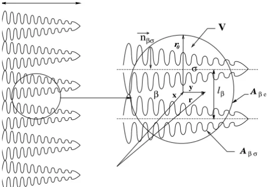
Finally, if Ake refers to the area of entrances and exits of the k-phase in V (Figure 1), the boundary conditions atAkeare:
vβ = Fv(r, t ) atAβe (12)
Ck = Hk(r, t ), k=β, σ atAσ e (13)
Tk = Ik(r, t ), k=β, σ atAσ e (14)
where the functionsFv, Hk andIk (k = β, σ) are unknown at this stage. The discussion concerning the nature of these functions will take place in section 3.
2.2 Geometrical considerations
The volume averaging method is an up-scaling method generally used for systems where the separation between the characteristic length scale is satisfied [21]. In columnar dendritic structures, averaged properties are actually continuously space-dependent and therefore scale separation depends on the spatial evolution of the geometry (decreasing rate of the geometryτ) [23]. Three length scale constraints have been identified (Table 1).
τ Length scale constraint
small ℓβ ≪ r0 ≪ L (15)
moderate ℓβ < r0 < L (16)
large ℓβ ≤ r0 ∼L (17)
Table 1 – Influence of the decreasing rateτ on the length-scale constraints [23].
etal. [23] show that, although less clear-cut, scale separation remains satisfied since:
lβ ≪L (18)
Under this condition, the averaging procedure can still be used but two difficul-ties arise. First, the averaged properdifficul-ties are not only point-dependent but also depend on the size of the averaging volume. Second, as shown later, porosity gradients explicitly appear both in the macroscopic conservation equations and in the associated closure problems giving rise to a very complex closure analysis (section 3).
2.3 Averaged equations
Keeping in mind condition (18), we now apply the classical averaging theorems to the system (1)–(14) after introducing Gray’s decomposition [33]:
k = kk+k k=β, σ (19)
where kk and k represent the intrinsic average and the deviation of the generic quantity in the k-phase, respectively. kk is obtained by using definition (A.3). This leads to the followingnon-closedmacroscopic equations.
2.3.1 Mass and momentum equations
Averaging the mass balance at the solid-liquid interface equation (8) gives rise to:
σ
k=β
˙
mk =0 (20)
wherem˙k is the melting (k=β) or the solidification (k=σ) rates defined by:
˙
mk = − 1 V
Aβσ
ρknβσ ·(vk−wβσ) dA (21)
neglected in this analysis. Therefore, the averaged mass conservation equation for the mixture takes the final form:
∂
∂t(εβρβ +εσρσ)+ ∇ ·(εβρβvβ β
)=0 (22)
while averaging Navier-Stokes equation (3) leads, after simplifications, to the non-closed averaged momentum equation:
∂ ∂t
εβρβvββ
+ ∇ ·εβρβvββvββ
+ ∇ ·εβρβvβvββ
+ 1
V
Aβσ
nβσ ·(vβ −wβσ)ρβvβ dA
= −εβ∇Pββ +εβµβ∇2vββ +εβρβg
+ 1
V
Aβσ
nβσ ·
−PβI+µβ∇vβ
dA
+ µβ∇ ·
1 V
Aβσ
nβσvβ dA
(23)
2.3.2 Concentration equations
As previously said, one originality of the present model lies in the macroscale non-equilibrium description of the solute transport. In other words, the solute transport is described separately in the liquid and solid phases and no partic-ular assumption is retained concerning the solute diffusion in the solid phase. Interfacial solute exchange due to the difference between interfacial- and volume-averaged concentrations in both phases are explicitly included in the analysis. Averaging equations (4) and (5) leads to the non-closed macroscopic equations for solute transport in the solid and liquid phases:
∂ ∂t
εσρσCσσ
+ 1
V
Aβσ
ρσCσnσβ ·(−wβσ) dA
= ρσεσ∇ ·
Dσ∇Cσσ
+ρσDσ
V
Aβσ
nσβ· ∇Cσ dA
+ ∇ ·
ρσDσ V
Aβσ
nσβCσ dA
∂
∂t(εβρβCβ
β)+ ∇ ·(ε
βρβCββvββ)+ ∇ ·
εβρβvβCββ
+ 1
V
Aβσ
ρβCβnβσ ·(vβ−wβσ) dA
= ρβεβ∇ ·
Dβ∇Cββ
+ρβDβ
V
Aβσ
nβσ · ∇Cβ dA
+ ∇ ·
ρβDβ V
Aβσ
nβσCβ dA
(25)
2.3.3 Energy equations
Similarly, averaging equations (6) and (7) leads the non-closed energy conser-vation equations:
∂
∂t(εσρσHσ σ
)+ 1
V
Aβσ
ρσHσnσβ·(−wβσ) dA
= ∇ ·(εσλσ∇Tσσ)+ λσ
V
Aβσ
nσβ· ∇Tσ dA
+ ∇ · λσ V Aβσ
Tσnσβ dA
(26)
∂
∂t(εβρβHβ β)+ 1
V
Aβσ
ρβHβnβσ ·(vβ−wβσ) dA
+ ∇ ·εβρβHββvββ
+ ∇ ·εβρβ ˜Hβvββ
= ∇ ·(εβλβ∇Tββ)+ λβ
V
Aβσ
nσβ· ∇Tβ dA
+ ∇ · λβ V Aβσ
Tβnσβ dA
Since the Lewis number (ratio of the thermal to the mass diffusivity) is high for metallic alloys (Le∼104), the liquid and solid phases are in thermal equilibrium
[2] and only one averaged energy equation can be used sinceTββ ≃ Tσσ ≃
T[34, 35]. Therefore, adding equations (26) and (27) and taking into account
the boundary condition (10), a single non-closed energy equation is obtained:
∂
∂t (ρH)+ ∇ ·
εβρβHββvββ
+ ∇ ·εβρβ ˜Hβvββ
= ∇ ·εβλβ +εσλσ
∇T
+ ∇ ·
1 V
Aβσ
λσTσnσβ+λβTβnβσ
dA
(28)
where H = (εβρβHββ +εσρσHσσ)/ρ represents the enthalpy of the mixture. Rigourously, equations (23)–(28) have been obtained after discard-ing numerous geometrical moments that have been shown to be very small in dendritic structures [23]. Let us only recall that the main consequence of this simplification is that the averaged quantities can be extracted from area integrals. In equations (23)–(25) and (28), the area integral terms involving the deviation quantities are actually related to effective transport properties of the dendritic mushy zone. In order to derive a closed form of these equations, the associated closure problems have to be written to express the deviation fieldsψk in terms of intrinsic averaged quantities kk.
3 Closure
The first step of the derivation of closure problems is performed by using the Gray’s decomposition in the local conservation equations (1)–(7) and by sub-tracting the non-closed averaged equations (23)–(25) and (28). This gives rise to a very complex set of deviation equations which can be simplified first by comparing the order of magnitude of the different terms on the basis of the length scale constraint (16), and second, by allowing for the following physical considerations:
(ii) The solidification process is slow enough to consider that the interface growth velocity is small compared to the average liquid velocity [36].
(iii) The time scales separation is satisfied and the deviation problems can be treated as quasi-steady [27].
(iv) Temperature and concentration at the interface can be decoupled at the closure-problem level [26].
The derivation of closure problems for homogeneous structures does not raise any major difficulty but the presence of evolving heterogeneities makes this derivation more complex. It order to illustrate this, let us consider the boundary value problem for deviationsPβ andvβ, which, after straightforward manipulations, takes the form:
∇ ·vβ =0 (29)
ρβvβ · ∇vβ = − ∇Pβ +µβ∇2vβ
− 1
V
Aβσ
nβσ ·(−PβI+µβ∇vβ) dA
− µβε−β1
∇εβ· ∇vββ + ∇2εβvββ
source term
(30)
vβ = − vββ
source term
atAβσ (31)
vβ = Fv(r, t ) atAβe (32)
properties. In that case, looking for a solution forPβ andvβ would impose a relation of the type:
Pβ,vβ =G(vββ,∇εβ,∇2εβ,∇vββ) (33) whereGis therefore related to the closure variables whose determination remains an extremely complicated task needing more theoretical developments. How-ever, if we consider the length scale constraint (18), we can estimate that the two last terms in equation (30) are small compared to the area integral friction term, leading to a classical boundary value problem [37]. This is obviously an ap-proximation since, due to evolving heterogeneities, (18) is not valid everywhere along the dendrites. The second difficulty concerns the nature ofFv(r, t )atAβe. For homogeneous porous media, the boundary value problem is generally solved in a representative region (unit cell) with periodicity conditions for pressure and velocity. In dendritic structures, a flow rate conservation condition would be probably more realistic. Nevertheless, it is known that the boundary condition (32) influences the deviation fields only on a region of thicknesslβat the bound-ary of the averaging volume [37]. Finally, unlike homogeneous porous media, averaged properties in dendritic structures not only depend on the location of the averaging volume but also depend on the size of this latter. Actually, this de-pendence is directly related to the decreasing rate of the structure geometry. For moderate evolving heterogeneities, it has been shown that a common range for r0exists where effective transport properties are rather constant [23, 24]. Taking
into account the above assumptions, the simplified problems for momentum, concentration and temperature deviations are finally given by:
Momentum
∇ ·vβ =0 (34)
ρβvβ· ∇vβ = −∇Pβ+µβ∇2vβ − 1 V
Aβσ
nβσ ·(−PβI+µβ∇vβ) dA (35)
vβ = − vββ
source term
atAβσ (36)
Concentration
Dσ∇2Cσ −ε−σ1
1 V
Aβσ
nσβ·Dσ∇Cσ dA =0 (38)
vβ· ∇Cβ +vβ· ∇Cββ
source term
=Dβ∇2Cβ −εβ−1
1 V
Aβσ
nβσ ·Dβ∇CβdA (39)
Ck =Ck∗− Ckk
source term
atAβσ (40)
Ck(r+ℓi)=Ck(r) with i =1,2,3 atAke (41)
Temperatures
λσ∇2Tσ −λσε−σ1
1 V
Aβσ
nσβ· ∇Tσ dA =0 (42)
ρβcpβvβ · ∇Tβ +ρβcpβvβ· ∇T
=λβ∇2Tβ −λβε−β1
1 V
Aβσ
nβσ · ∇Tβ dA
(43)
λσnσβ· ∇Tσ −λβnσβ · ∇Tβ =
λβ−λσ
nσβ· ∇T
source term
atAβσ (44)
Tσ =Tβ atAβσ (45)
Tk(r+ℓi)=Tk(r) with i=1,2,3 atAke (46)
whereCk∗in condition (40) represents the average concentration in thek-phase at the interface. In the above system, let us recall that we requirekk = 0, where k represents a generic deviation field. The form of the macroscopic source terms in equations (36), (39), (40) and (44) generating the deviationsvβ,
Pβ, Ck andTk (k = β, σ), respectively, suggests that they can be written as [26, 27, 36, 37]:
vβ = M· vββ (47)
Cσ = ασ(Cσ∗− Cσσ) (49)
Cβ = bβ· ∇Cββ +αβ(Cβ∗− Cββ) (50)
˜
Tk = ekT k=σ, β (51)
whereM,m,αk, andekare the closure variables solutions of the periodic prob-lems which are obtained by introducing deviations (47)–(51) in the deviations problems (34)–(46). Since the closure problem (34)–(37) is non linear, it has been shown that the closure variableMcan be separated into a linear and inertia contributions, the former being related to the permeability tensor while the sec-ond one is related to the Forchheimer coefficient [37]. For conciseness, the set of periodic boundary closure problems are not detailed here, all the details being available in the following references [26, 36–40].
4 Closed form of the macroscopic model
According to assumptions (i)–(iv) and solutions (47)–(51), the final form of the macroscopic model for solidification of columnar dendritic mushy zone can be written:
∂
∂t(εβρβ)+ ∇ ·(ρβvβ)= − ∂
∂t(εσρσ)
solidification rate
(52)
εβ−1∂
∂t(ρβvβ)+ε
−1
β ∇ ·
ε−β1ρβvβvβ
= − Pββ+ρβg−µβK−1· vβ +µβεβ−1∇
2 vβ
− µβεβ−1∇εβ· ∇(ε−β1vβ)
second Brinkman correction term
− µβK−1·F· vβ
Forchheimer correction term
(53)
∂
∂t(εσρσCσ σ
)−Cσ∗ ∂
∂t(εσρσ)=εσ∇ ·(ρσDσ∇Cσ σ
)
+ρσhmσ(Cσ∗− Cσσ)
interfacial mass exchange
−∇ ·ρσDσ(∇εσ)(Cσ∗− Cσσ)
∂
∂t(εβρβCβ
β)+ ∇ ·(ρ
βCββvβ)−Cβ∗ ∂
∂t(εσρσ)
+ ∇ · [ρβdβ(Cβ∗− Cββ)] −ρβuβ· ∇Cββ
= ∇ ·(ρβDβ · ∇Cββ)−ρβDβ(∇εβ)· ∇Cββ
+ ρβhmβ(Cβ∗− Cββ)
interfacial mass exchange
−∇ ·ρβDβ(∇εβ)
Cβ∗− Cββ
(55)
∂
∂t (ρH)+ ∇ ·
ρβHββvβ
= ∇ ·eff∇T
(56)
where the velocity is written in term of superficial velocity (filtration). The solidification rate present in equations (52),(54) and (55) is obtained by averaging the boundary condition (9) to give:
(Cβ∗−Cσ∗)∂
∂t(εσρσ)=ρσhmσ(C
∗
σ − Cσσ)+ρβhmβ(Cβ∗− Cββ)
+ρβuβ · ∇Cββ−ρσ(∇εσ)·Dσ∇Cσσ
−ρβ(∇εβ)·Dβ∇Cββ
(57)
In equations (53)–(56),K,F,Dβ,eff andhmk(k=β, σ) represent the effective transport properties of the dendritic structure which are obtained after numerical determination of closure variable fields. In the momentum equation (53),Kis the permeability tensor that depends on the tortuosity of the porous structure whileF
represents the Forchheimer correction tensor which accounts for the local inertia effects. Since the closure variablesMandmin (47) and (48), respectively, have been decomposed in order to separate linear friction and inertia effect such as
M=R+S andm=r+s [37], KandF can be explicitly written under the form:
εβK−1= − 1 Vβ
Aβσ
nβσ ·(−Ir+ ∇R) dA (58)
ε2βK−1·F= − 1
Vβ
Aβσ
At this stage, the numerical solution of the closure problem for variablesSand
sassociated with the Forchheimer coefficient still remains a challenge. Dβ in equation (55) represents the effective diffusion dispersion tensor given by:
Dβ =εβDβI
Diffusion
− ˜vβbβ
Dispersion
(60)
while the effective conductivity in equation (56) is:
eff =(εσλσ +εβλβ)I+
(λβ −λσ) V
Aβσ
nσβ·eβ dA
Tortuosity
−ρβcpβ ˜vβeβ
Dispersion
(61)
Finally, in equations (54) and (55) the interfacial mass exchange due to macro-scale non-equilibrium is represented by two terms involving mass exchange coefficientshmk(k=β, σ) whose dependence to the local geometry is given by:
hmk = 1 V
Aβσ
nβσ ·Dk∇αk dA, k=β, σ (62)
5 Discussion and conclusion
second Brinkman correction term in the momentum equation (53). Although they can be considered as second order terms, all of them have to be quantified in the context of solidification before any conclusion concerning their contribu-tion on macroscopic transport phenomena may be drawn. Finally, it can be seen in equations (55) and (57) that other additional terms involvinguβ anddβ are included. Actually, these coefficients given by:
uβ = 1 V
Aβσ
nβσ ·Dβ∇bβ dA (63)
dβ = ˜vβαβ (64)
can be viewed as velocity-like vectors that contribute to macroscopic convective solute transport [27, 41, 42]. According to results obtained in the context of soil contamination, these terms are not necessarily negligible since they have been found to represent about 10% of the global convective transport [27].
In conclusion, the derivation of this solidification model using the method of volume averaging with closure has allowed us to provide a more complete macroscopic description of transport phenomena, improving the micro-macro interactions both in the definition of average transport properties and conservation equations. Numerical calculations are presently under development in order to quantify the relevance of such a model.
Appendix A – Volume-averaging definitions
If we consider a physical quantity β associated to theβ-phase, thesuperficial volume average of β in the averaging volumeV (Figure 1) is given by:
β =
1 V
Vβ
(x+y) dV (A.1)
whereVβ is the volume of theβ-phase contained within the averaging volume. In most cases, theintrinsicphase average of β is more representative and is defined by:
ββ =
1 Vβ
Vβ
Therefore,superficial and intrinsic averages are related by:
β =εβ ββ (A.3)
whereεβ is theβ-phase volume fraction.
Finally, averaged conservation equations can be obtained by using spatial and temporal partial derivative theorems given by [21]:
∇ β = ∇ β + 1
V
Aβσ
nβσ βdA (A.4)
∂ β ∂t
= ∂ β
∂t −
1 V
Aβσ
nβσ ·wβσ βdA (A.5)
where wβσ is the interface velocity and nβσ is the unit normal vector at the solid-liquid interface (Figure 1) [21].
βe A
Aβ σ
lβ
r0
βσ
n
x r y
β
σ
L
V
Figure 1 – Macroscopic dendritic mushy zone and an associated averaging volume.
Nomenclature
Aβσ interfacial area of theβ-σ interface within the macroscopic region, m2. Ake area of entrances and exits for thek-phase within the macroscopic
Ck concentration in thek-phase, wt pct.
Ck∗ average concentration at the interface, wt pct. Dk molecular diffusivity of thek-phase, m2s−1.
Dβ effective solute dispersion tensor, m2s−1.
dβ a velocity vector-like coefficient, ms−1.
F Inertia tensor
g gravitational acceleration, m.s−2. hmk mass exchange coefficient, s−1. Hk enthalpy in thek-phase.
I unit tensor.
K permeability tensor, m2
L general characteristic lengh for volume averaged quantities, m. lβ interdendritic lengh scale and size of the unit cell, m.
li i= 1,2,3 lattice vectors, m.
˙
mk phase change rate, kg m−3s−1.
nβσ unit normal vector pointing from theβ-phase toward theσ-phase. Pβ pressure in theβ–phase, Pa.
r0 size of the averaging volume, m.
Tk Temperature in thek-phase , K. t time, s
t time scale for deviation quantity, s t∗ time scale for average quantity, s
uβ a velocity vector-like coefficient, ms−1. V averaging volume, m3.
Vk volume of thek-phase withinV, m3.
vβ velocity vector in theβ-phase, ms−1.
vβ superficial averaged velocity, ms−1.
wβσ interface velocity vector, ms−1. Greek Letters
εk k-phase volume fraction.
eff Effective conductivity, W m−1K−1. µβ dynamic viscosity of theβ–phase, Pa.s.
kk intrinsic average of the quantity k . ρk k-phase density, Kg m−3.
Subscripts
β liquid phase σ solid phase
REFERENCES
[1] C. Beckermann and R. Viskanta, Applied Mechanics Review46(1) (1993), 1–27. [2] C. Beckermann and C.Y. Wang, Annual Review of Heat Transfer6(1995), 115–198. [3] P.J. Prescott and F.P. Incropera, Adv. in Heat Transfer28(1996), 231–338.
[4] R.N. Hills, D.E. Lopper and P.H. Roberts, Q.J. Mech. appl. Math.36(1983), 505–539. [5] W.D. Bennon and F.P. Incropera, Int. J. Heat Mass Transfer30(10) (1987), 2161–2170. [6] P.J. Prescott, F.P. Incropera and W.D. Bennon, Int. J. Heat Mass Transfer34 (9) (1991),
2351–2359.
[7] C. Beckermann, Melting and solidification of binary mixtures with double-diffuse convection in the melt, Ph.D. thesis, Purdue University, West Lafayette (1987).
[8] S. Ganesan and D.R. Poirier, Metallurgical Transactions21B(1990), 173–181. [9] J. Ni and C. Beckermann, Met. Trans.22B(1991) 349–361.
[10] C.Y. Wang and C. Beckermann, Met. Trans.A 24A(1993) 2787–2802.
[11] C.Y. Wang and C. Beckermann, Metallurgical and Material TransactionsA 27A(1996), 2754–2764.
[12] N. Streat and F. Weinberg, Met. Trans. B7B(1976), 417–423.
[13] K. Murakami, A. Shiraishi and T. Okamoto, Acta metall.31(1983), 1417–1424. [14] R. Nasser-Rafi, R. Deshmukh and D.R. Poirier, Met. Trans.16A(1985), 2263–2271. [15] D.R. Poirier, Met. Trans.18B(1987), 245–255.
[16] C. Beckermann and R. Viskanta, Physico Chemical Hydrodynamics,10(1988), 195–213. [17] S. Ganesan, C.L. Chan and D.R. Poirier, Materials Science and EngineeringA151(1992),
97–105.
[18] D.R. Poirier and P. Ocansey, Materials Sciences and EngineeringA171(1993), 231–240. [19] M.S. Bhat, D.R. Poirier and J.C. Heinrich, Metallurgical and Materials TransactionsB
[20] M.C. Schneider and C. Beckermann, Int. J. Heat Mass Transfer38(18) (1995), 3455–3473. [21] S. Whitaker, Ind. Eng. Chem.12(1969), 12–28.
[22] J. Bear, Dynamics of Fluids in Porous Media, Dover, (1972).
[23] B. Goyeau, T. Benihaddadene, D. Gobin and M. Quintard, Transport in Porous Media
28(1997), 19–50.
[24] B. Goyeau, T. Benihaddadene, D. Gobin and M. Quintard, Metallurgical and Materials TransactionsB 30B(1999), 613–622.
[25] A. Neculae, B. Goyeau, M. Quintard and D. Gobin, Mat. Eng. SciencesA 323(2002), 367–376.
[26] P. Bousquet-Melou, A. Neculae, B. Goyeau and M. Quintard, Metallurgical and Materials TransactionsB 33B(2002), 365–376.
[27] M. Quintard and S. Whitaker, Advances in Water Resources17(1994), 221–239.
[28] S. Whitaker, The Method of Volume Averaging, Vol. 13, Kluwer Academic Publishers, 1999. [29] J. Cushman, Water Resources Research20(11) (1984), 1668–1676.
[30] J.A. Ochoa-Tapia and S. Whitaker, Int. J. Heat Mass Transfer38(1995), 2635–2646. [31] J.A. Ochoa-Tapia and S. Whitaker, Int. J. Heat Mass Transfer38(1995), 2647–2655. [32] J.A. Ochoa-Tapia and S. Whitaker, Int. J. Heat Mass Transfer40(1998), 2691–2707. [33] W.G. Gray, Chem. Eng. Sci.3(1975), 229–233.
[34] S. Whitaker, Transport in Porous Media1(1986), 3–35.
[35] M. Quintard and S. Whitaker, Int. J. Heat Mass Transfer38(15) (1995), 2779–2796. [36] P. Bousquet-Melou, B. Goyeau, M. Quintard, F. Fichot and D. Gobin, Int. J. Heat Mass
Transfer45(2002), 3651–3665.
[37] S. Whitaker, Transport in Porous Media25(1996), 27–61.
[38] M. Quintard, M. Kaviany and S. Whitaker, Advances Water Resources20(2-3) (1997), 77–94.
[39] P. Bousquet-Melou, Modélisation macroscopique et simulation numérique de la solidification des mélanges binaires, Ph.D. thesis, University of Paris 6 (2000).
[40] C. Moyne, S. Didierjean, H.P. Amaral-Souto and O.T. da Silveira, Int. J. Heat Mass Transfer
43(2000), 3853–3867.
![Table 1 – Influence of the decreasing rate τ on the length-scale constraints [23].](https://thumb-eu.123doks.com/thumbv2/123dok_br/18977843.455933/5.918.257.661.816.945/table-influence-decreasing-rate-τ-length-scale-constraints.webp)