Tropical Pacific spatial trend patterns in observed sea level: internal variability and/or anthropogenic signature?

(1)

CPD

8, 349–389, 2012

Tropical Pacific spatial trend patterns in observed sea level

B. Meyssignac et al.

Title Page

Abstract Introduction

Conclusions References

Tables Figures

◭ ◮

Back Close

Full Screen / Esc

Printer-friendly Version Interactive Discussion

Discussion

P

a

per

|

Dis

cussion

P

a

per

|

Discussion

P

a

per

|

Discussio

n

P

a

per

Clim. Past Discuss., 8, 349–389, 2012 www.clim-past-discuss.net/8/349/2012/ doi:10.5194/cpd-8-349-2012

Climate of the Past Discussions

This discussion paper is/has been under review for the journal Climate of the Past (CP). Please refer to the corresponding final paper in CP if available.

Tropical Pacific spatial trend patterns in

observed sea level: internal variability

and/or anthropogenic signature?

B. Meyssignac1, D. Salas y Melia2, M. Becker1,*, W. Llovel3, and A. Cazenave1

1

LEGOS/CNES, UMR5566, 14, avenue E. Belin, 31400 Toulouse, France

2

M ´et ´eo-France CNRM/GMGEC CNRS/GAME, 31000 Toulouse, France

3

JPL, California Institute of Technology, Pasadena, California, USA

*

now at: University of Cayenne, Guyane, France

Received: 12 December 2011 – Accepted: 6 January 2012 – Published: 13 January 2012 Correspondence to: B. Meyssignac ([email protected])

(2)

CPD

8, 349–389, 2012

Title Page

Tables Figures

◭ ◮

Back Close

Full Screen / Esc

Discussion

P

a

per

|

Dis

cussion

P

a

per

|

Discussion

P

a

per

|

Discussio

n

P

a

per

|

Abstract

We investigate the spatio-temporal variability of sea level trend patterns observed by satellite altimetry since 1993, focusing on the Tropical Pacific. The objective of this study is two fold. On the basis of a 2-D past sea level reconstruction (over 1950–2009) – based on a combination of observations and ocean modelling – and multi-century 5

control runs (i.e. with constant, preindustrial external forcing) from eight coupled cli-mate models, we investigate how these sea level trend patterns evolved during the last decades and centuries, and what their characteristic time scales are. Using 20th cen-tury coupled climate model runs, we also examine whether observed trend patterns are driven by external forcing factors (i.e. solar plus volcanic variability and changes 10

in anthropogenic forcing) or if they essentially result from natural climate variability. For this analysis, we computed sea level trend patterns over successive 17 yr win-dows (i.e. the length of the altimetry record) both for the reconstructed sea level and model runs. We compared them to altimetry-based observed trends. The 2-D sea level reconstruction shows similar spatial trend patterns to those observed during the 15

altimetry era. The patterns appear to have fluctuated with time with a characteristic time scale of the order of 25–30 yr. Similar behaviour is found in multi-centennial con-trol runs of the coupled climate models. The same analysis, performed on 20th century model runs does not display significant differences. This suggests that Tropical Pacific sea level trend fluctuations are still dominated by the internal natural variability of the 20

ocean-atmosphere coupled system. While our analysis cannot rule out any influence of anthropogenic forcing, it concludes that the latter effects on the regional sea level patterns are still hardly detectable.

1 Introduction

Long term sea level rise is a critical issue of the global climate change because of its 25

(3)

CPD

8, 349–389, 2012

Title Page

Tables Figures

◭ ◮

Back Close

Full Screen / Esc

Discussion

P

a

per

|

Dis

cussion

P

a

per

|

Discussion

P

a

per

|

Discussio

n

P

a

per

For this reason, it has been extensively studied in recent years. Since 1993, sea level is accurately monitored by satellite altimetry (using the Topex/Poseidon, 1, Jason-2, ERS-1/2 and Envisat satellite missions) with high accuracy and global coverage. Recent studies based on these observations showed that sea level is rising at a global mean rate of 3.3 mm yr−1

since 1993 (e.g. Ablain et al., 2009; Cazenave and Llovel, 5

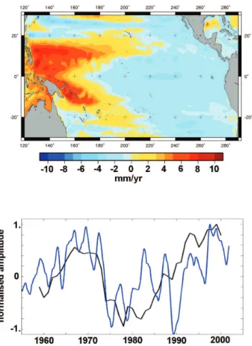
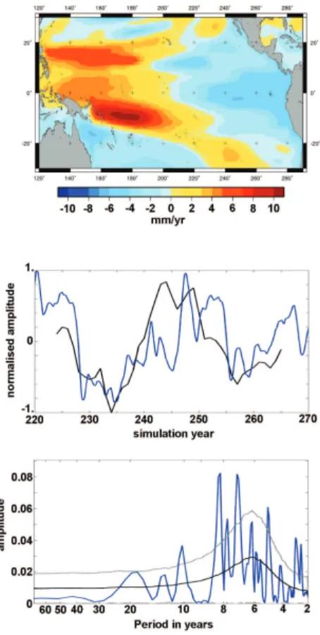
2010; Nerem et al., 2010). They showed as well that sea level does not rise uniformly but displays strong regional variability (see Fig. 1a). To highlight this regional variability,

the uniform trend (global mean) of 3.3 mm yr−1

has been removed from Fig. 1a. In some regions such as the Western Pacific, the North Atlantic around Greenland, or the South-Eastern Indian sea level rose up to 4 times faster than the global mean over 10

1993–2009. Meanwhile, other regions such as the Eastern Pacific or North-Western Indian Ocean show lower rates of sea level rise. These large deviations from the global mean trend suggest that in different parts of the world, low lying lands are not facing the same risk at sea level rise. Hence, when assessing the potential impacts of sea level rise, it is of primary importance to understand the time variability of observed regional 15

sea level trend patterns and the causes which drive them.

A number of previous studies have shown that sea level trend patterns over the

al-timetry era mainly result from ocean temperature and salinity changes (e.g. Bindoff

et al., 2007). This was evidenced by the comparison between altimetry-based and steric trend patterns deduced from in-situ hydrographic measurements (Ishii and Ki-20

moto, 2009; Levitus, 2005; Levitus et al., 2009; Lombard et al., 2005a,b) and ocean general circulation models (OGCMs) outputs (Wunsch et al., 2007; Kohl and Stam-mer, 2008; Carton and Giese, 2008; Lombard et al., 2009). Analyses of in situ ocean temperature measurements showed that the thermosteric component is the most im-portant contribution to the observed sea level regional variability. OGCM runs with or 25

without data assimilation have confirmed that point. However salinity changes may also

play some role at regional scale, partly compensating temperature effects, as shown

(4)

CPD

8, 349–389, 2012

Title Page

Tables Figures

◭ ◮

Back Close

Full Screen / Esc

Discussion

P

a

per

|

Dis

cussion

P

a

per

|

Discussion

P

a

per

|

Discussio

n

P

a

per

|

Other phenomena may also contribute to the regional variability in rates of sea level

change. This is the case of gravitational and deformational effects associated with

the last deglaciation and ongoing land ice melting (Gomez et al., 2010; Milne and Mitrovica, 2008; Milne et al., 2009; Mitrovica et al., 2001, 2009). However these effects are currently small and have not yet been detected in the altimetry-based sea level 5

patterns.

Observations have shown that thermosteric spatial patterns are not stationary but fluctuate with time in response to driving mechanisms such as ENSO (El Nino-Southern Oscillation), NAO (North Atlantic Oscillation) and PDO (Pacific Decadal Os-cillation) (Levitus, 2005; Lombard et al., 2005a; Di Lorenzo et al., 2010; Lozier et al., 10

2010). Thus regional sea level trend patterns observed over the altimetry era were likely different prior to 1993.

The spatial and temporal variability of steric sea level change is tightly linked to complex ocean dynamics. It results from the redistribution of heat and fresh water both horizontally and vertically through sea-air fluxes and changes in the ocean circulation. 15

Several studies have identified surface wind stress as the main driving mechanism of circulation-based heat and salt redistribution over the past few decades (e.g. Kohl and Stammer, 2008), in particular in the Equatorial Pacific Ocean (Timmermann et al., 2010). But according to Kohl and Stammer (2008), surface fluxes and particularly buoyancy fluxes may have played an increasing role during the past 2 decades. 20

This important role of heat and fresh water redistribution in steric sea level trend patterns was previously noticed by Wunsch et al. (2007). They argued that given the long memory time of the ocean, observed patterns reflect an integration of the forcing patterns of the considered period with forcing and internal changes that occurred earlier in the past. This is another argument which suggests that the sea level trend patterns 25

(5)

CPD

8, 349–389, 2012

Title Page

Tables Figures

◭ ◮

Back Close

Full Screen / Esc

Discussion

P

a

per

|

Dis

cussion

P

a

per

|

Discussion

P

a

per

|

Discussio

n

P

a

per

characteristic time scales?, (2) What are the factors that drive them: are they mainly due to internal variability of the climate system or can we detect some imprint of exter-nal forcing factors, in particular anthropogenic forcing?

2 Methods

In this study we focus on the sea level spatial trend patterns of the Tropical Pacific. 5

To try to answer the above questions concerning this region, we use different

obser-vational data sets and climate model outputs. For the sea level observations we use altimetry data since 1993 and a new version of a past sea level reconstruction over 1950–2009 (Meyssignac et al., 2012). For the climate models outputs, we use runs of eight coupled global climate models (CGCM here after) from the Coupled Model 10

Intercomparison Project 3 database (hereafter CMIP3). These datasets are presented hereafter in more details.

Using the altimetry data set, we compute the observed spatial trend patterns over 1993–2009. Using the reconstructed 2-D sea level fields since 1950, we compute sea level trend patterns over successive 17 yr windows (the length of the altimetry data set) 15

for the past decades. The objective is to identify the dominant modes of variability and the characteristic life time of the 17 yr observed spatial trend patterns over the last 60 yr. Then we compute, the sea level trend patterns over successive 17 yr windows from the CGCM multi-centennial control run outputs. These runs with constant, preindustrial external forcing give us an estimation of the modelled 17 yr sea level trend patterns 20

produced by the internal variability of the climate system and their evolution with time. We check whether the Tropical Pacific sea level trend patterns resemble those seen in the observations or not. A similar analysis is done with the CGCM climate model runs over the 20th century. All these runs represent the human-induced changes in atmospheric greenhouse gases and aerosols. As discussed later in this paper, some 25

(6)

CPD

8, 349–389, 2012

Title Page

Tables Figures

◭ ◮

Back Close

Full Screen / Esc

Discussion

P

a

per

|

Dis

cussion

P

a

per

|

Discussion

P

a

per

|

Discussio

n

P

a

per

|

the anthropogenic forcing changes and the variability of natural forcing factors already have a visible imprint on the time variability of the 17 yr sea level trend patterns during the 20th century.

3 Data

3.1 Satellite altimetry sea level data (1993–2009) 5

We used altimetry-based 2-D sea level fields from AVISO (http://www.aviso.oceanobs. com/en/data/products/sea-surface-height-products/global/index.html). The data

con-sists of gridded sea level anomalies at weekly interval on a 1/4◦ _{regular grid, from}

January 1993 to December 2009. We used the DT-MSLA “Ref” series computed at CLS (Collecte Localisation Satellite) by combining several altimeter missions, namely: 10

Topex/Poseidon, Jason 1 and 2, Envisat and ERS 1 and 2. It is a global homoge-nous intercalibrated dataset based on global crossover adjustment (Le Traon and Ogor, 1998) using Topex/Poseidon and then Jason 1 as reference missions. It is corrected for the long wavelength orbit errors (Le Traon et al., 1998), ocean tides, and wet/dry troposphere and ionosphere (see Ablain et al., 2009 for more details). The inverted 15

barometer (IB) correction has also been applied in order to minimize aliasing e_ffects

(Volkov et al., 2007) through the MOG2D barotropic model correction that includes

the dynamic ocean response to short-period (<20 day) atmospheric wind and pressure

forcing and the static IB correction at periods above 20 day (see Carrere Lyard, 2003 for details).

20

3.2 Two-dimensional past sea level reconstruction (1950–2009)

(7)

CPD

8, 349–389, 2012

Title Page

Tables Figures

◭ ◮

Back Close

Full Screen / Esc

Discussion

P

a

per

|

Dis

cussion

P

a

per

|

Discussion

P

a

per

|

Discussio

n

P

a

per

et al. (2009)’s reconstruction. The method, based on the reduced optimal interpolation described by Kaplan et al. (2000), consists of interpolating (2-D interpolation) long tide gauge records with a time varying linear combination of spatial patterns of a 2-D sea level field. The method has 2 steps. In the first step an Empirical Orthogonal Function (EOF) decomposition (Preisendorfer, 1988; Toumazou and Cretaux, 2001) of 2-D sea 5

level fields is done (based on outputs of the OPA/NEMO ocean circulation model). This decomposition allows separating the spatially well resolved signal of the model into spatial modes (EOFs) and their related principal component (PC). The second step consists of computing new PCs over a longer period (1950–2003) covered by the selection of the considered 99 long tide gauge records. It is done through a least 10

square optimal procedure that minimizes the di_fference between the reconstructed field

and the tide gauge records at the tide gauge locations. Compared to the previous sea level reconstruction of Church et al. (2004), the originality of the Llovel et al. (2009)’s reconstruction is the use of long-term sea level patterns (EOFs) deduced from a 44 yr long run of the OPA/NEMO ocean model instead of the shorter altimetry record. This, 15

in principle, allows better capturing the decadal variability of the spatial trend patterns (see Llovel et al., 2009 for more details).

In the present study, we use a new version of the reconstruction based on three modifications. First, we followed Christiansen et al. (2010) and made use of a covari-ance matrix error and the so called EOF0 (i.e. the EOF mode corresponding to the 20

geographically averaged but time variable sea level, processed separately from the other EOF modes as in Church et al. 2004’s reconstruction). This drastically improves the accuracy of the reconstructed trends over the reconstructed period. Second, on the basis of the lastest data available from the PSMSL (Permanent Service For Mean Sea Level: http://www.psmsl.org), we updated the tide gauge records used by Llovel 25

et al. (2009) and reconstructed sea level until December 2009. Thus the new recon-struction provides a global 2-D spatial field of sea level every month from January 1950 to December 2009. Third, for the computation of the EOFs patterns, instead

(8)

CPD

8, 349–389, 2012

Title Page

Tables Figures

◭ ◮

Back Close

Full Screen / Esc

Discussion

P

a

per

|

Dis

cussion

P

a

per

|

Discussion

P

a

per

|

Discussio

n

P

a

per

|

preferred to use the ORCA025-B83 run of the DRAKKAR/NEMO model which has a higher resolution of 1/4◦

. Indeed, Penduffet al. (2010) showed that ocean models

with higher resolution bring substantial improvements in the representation of the sea level spatial variability, in particular at interannual time scales. The ORCA025-B83 run is based on the free surface ocean circulation model NEMO version 2.3 (Madec, 2008). 5

This simulation is very close to the simulation ORCA025-G70 analysed and compared to altimetry by Lombard et al. (2009). It does not assimilate any observational data (e.g. satellite altimetry or in situ data) as in ORCA025-G70. It is also forced by the more realistic hybrid surface forcing “DRAKKAR forcing set 4.1” described in details by Brodeau et al. (2010). This forcing is based on the CORE dataset assembled by 10

W. Large (Large and Yeager, 2004), the ECMWF (European Center for Medium-Range Weather Forecast) ERA 40 reanalysis (Uppala et al., 2005) and the ECMWF opera-tional analyses for the recent years. This new reconstruction has been validated at global scale (Meyssignac et al., 2012) and in the Tropical Pacific region (Becker et al., 2012) by comparison with independent tide gauges not used in the reconstruction pro-15

cess. Figure 1b shows the reconstructed sea level trend patterns over 1950–2009.

As expected, regional sea level trend patterns reconstructed over the last 60 yr di_ffer

largely from those observed during the last 17 yr (see Fig. 1a for comparison).

3.3 Coupled climate models (CGCM) runs

Concerning the CGCM simulations, we both analysed multi-centennial control runs 20

(named picntrl run in the CMIP3 nomenclature) and runs covering the 20th century (20c3m run in the CMIP3 nomenclature) starting in the mid 19th century and ending in the 2000s.

The control runs and the 20th century runs di_ffer in the external forcing. The external forcing includes changes in greenhouse gases, tropospheric and stratospheric ozone, 25

(9)

CPD

8, 349–389, 2012

Title Page

Tables Figures

◭ ◮

Back Close

Full Screen / Esc

Discussion

P

a

per

|

Dis

cussion

P

a

per

|

Discussion

P

a

per

|

Discussio

n

P

a

per

to provide an estimate of the internal variability of the climate system. The 20c3m runs provide an estimate of the 20th century climate. They use observed, time-varying external forcing from around 1860 to 2000.

Among all CGCM available in CMIP3, we have selected models providing that both the sea surface temperature and the sea level variables were available in their control 5

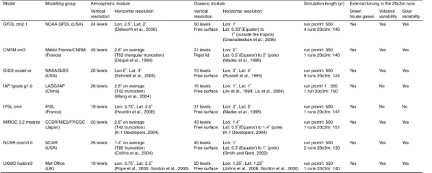
run and 20th century run outputs. Models with less than 300 yr of control run were discarded. This led us to use a subset of 8 models: GFDL cm2.1, CNRM cm3, GISS model er, IAP fgoals 1.0, IPSL cm4, MIROC 3.2 medres, NCAR ccsm3.0 and UKMO hadcm3. The vertical and horizontal resolutions for the atmospheric and oceanic mod-ules of each model are gathered in Table 1 along with the references in which they are 10

described in details. Note that for each of the selected models one control run and one 20th century run at least were analyzed. When several 20th century runs were avail-able (see Tavail-able 1), they were all analyzed one by one. Note as well that the selected

models di_ffer in their external forcing of the 20c3m runs. The IPSL cm4 20c3m run

does not include the solar and volcanic variability and the IAP fgoals g1.0 20c3m does 15

not include the volcanic variability (see Table 1) while other models do. But we decided to keep them in our selected subset anyway because few models provide the outputs necessary for this study, and we chose not to reduce this set further. However the final discussion will show that it does not impact our conclusions.

The sea surface height (SSH) fields given in the model outputs are incomplete and 20

can not be directly compared to the observations in terms of global mean. Indeed they do not contain the global mean steric sea level signal since they are computed for all models on the basis of the Boussinesq assumption that enforces the total ocean volume to remain constant. But apart from such unrealistic global mean, the models correctly simulate the regional sea level changes because the Boussinesq assumption 25

(10)

CPD

8, 349–389, 2012

Title Page

Tables Figures

◭ ◮

Back Close

Full Screen / Esc

Discussion

P

a

per

|

Dis

cussion

P

a

per

|

Discussion

P

a

per

|

Discussio

n

P

a

per

|

4 Results

All computations were done on the basis of the monthly time series from altimetry, the 2-D past reconstruction and the CGCMs. In this study we are interested in the regional variations of the sea level trends at inter-annual to multi-decadal time scales. Hence 2 calculations have been applied to the sea level time series prior to our analysis. (1) The 5

global mean sea level trend was removed from the sea level time series because this study focuses on the regional variability around the global mean (this also removes in the same time any internal drift of the CGCM runs). (2) The time series were averaged to annual time series and filtered for the multi-centennial signals to focus on the inter-annual to the multi-decadal time scales. These low frequency signals were filtered 10

out with a high-pass filter with a 80 yr cuto_ff. The high pass filter built here is a fast

Fourier transform convolution with a Hamming window cutting at 1/80 yr−1_(Brigham,

1974). The choice of the 80 yr filter cutoffenables to keep all the variability with period lower than 70 yr, in which we are most interested (see further), and to ensure a reliable (somewhat conservative) filtering of the multi-centennial signals.

15

4.1 Observed Tropical Pacific 17 yr trend patterns since 1950

Over the 17 yr of altimetry era, sea level trends show characteristic patterns (see Fig. 1a). The most prominent feature is the strong ENSO-like dipole in the Tropical Pacific region which is positive in the western part and negative in the eastern part. This pattern has been persistent for several years now. It was already observed over 20

the first 10 yr of the altimetry period (1993–2003) by Cazenave and Nerem (2004) (see their Fig. 7). With the 2-D past sea level reconstruction we can gain some insights on how the sea level trend patterns evolved over longer time scales (here, up to 60 yr). We computed spatial trend patterns of reconstructed sea level over successive 17 yr windows (i.e. the length of the altimetry data set). This gives as an output a set of 25

(11)

CPD

8, 349–389, 2012

Title Page

Tables Figures

◭ ◮

Back Close

Full Screen / Esc

Discussion

P

a

per

|

Dis

cussion

P

a

per

|

Discussion

P

a

per

|

Discussio

n

P

a

per

trend patterns over three time spans: 1993–2009, 1976–1992 and 1959–1975. They all three exhibit a strong ENSO-like dipole pattern. As expected, we note that the 1993– 2009 reconstructed sea level patterns are very close both in shape and amplitude to

the altimetry observed ones. The 1959–1975 trend patterns are somehow different

in shape but still exhibit a strong ENSO-like pattern with slightly lower amplitude than 5

over 1993–2009. The 1976–1992 patterns are opposed to the 1993–2009 ones almost everywhere. This indicates that trend patterns similar to presently observed ones, al-ready existed in the late 1960s and the early 1970s. They seem to have fluctuated with time and were opposite to present in the late 1970s and the 1980s. To investigate this further, we computed the EOF decomposition of the set of 43 reconstructed “17 yr” 10

trend maps. On the basis of these EOFs, we computed the first rotated EOF (see von Storch and Zwiers, 1999) to obtain the EOF that maximizes the variance explained among the 43 “17 yr” trend maps. This EOF is presented on Fig. 3. It accounts for most of the variance: 37 % of the total variance. The second rotated EOF explains 25 % of the total variance and the third one 7 %. The leading EOF spatial pattern is 15

very similar to the altimetry spatial pattern (Fig. 1a). This shows that the spatial pattern observed by satellite altimetry during the last 17 yr turn out to be the most frequently observed pattern among all the “17 yr” sea level trend maps of the last 60 yr (in terms of explained variance). Its PC indicates that this pattern has fluctuated with time (see Fig. 3). It was opposite to its current value in the 1970s and early 1980s and went 20

back to values similar to what we observe now in the late 1960s (with a lower am-plitude) as already suggested by Fig. 2. These fluctuations follow the low frequency variations of the extended NINO3 index (a proxy of El Nino) from Kaplan et al. (1998). This index is the average of the sea surface temperatures (SST) over the NINO3 region

(150◦_W–90◦_{W, 5}◦_S–5◦_{N). Here it has been smoothed out with a 10 yr running mean}

25

(12)

CPD

8, 349–389, 2012

Title Page

Tables Figures

◭ ◮

Back Close

Full Screen / Esc

Discussion

P

a

per

|

Dis

cussion

P

a

per

|

Discussion

P

a

per

|

Discussio

n

P

a

per

|

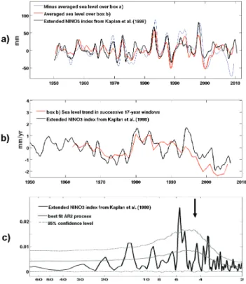
Another way to analyse the reconstructed 17 yr trend dipole fluctuations of the Trop-ical Pacific is to look at two regions defined by boxes A and B (see Fig. 2). Box A is

located in the Western Pacific (15◦_N–15◦_{S by 120}◦_E–200◦_{E) and box B in the}

East-ern Pacific (15◦_N–15◦_{S by 200}◦_E–280◦_{E). We computed the mean sea level (global}

mean sea level trend removed) in each box and compared it to the extended NINO3 5

index. The resulting curves are presented in Fig. 4a. Mean sea level in box A (Western Pacific) co-varies (but with opposite sign) with mean sea level in box B (Eastern Pa-cific). This confirms that the Tropical Pacific sea level behaves as an east-west dipole that fluctuates with time. This fluctuation follows closely the ENSO mode of variability represented by the NINO3 index: the correlation between NINO3 index and Eastern 10

Pacific mean sea level is 0.73 (SL>99 %). We have computed as well the mean sea

level trend in box B over successive 17 yr windows. Its time amplitude is displayed in Fig. 4b along with the NINO3 index time series smoothed with a 10 yr running mean. As suggested by the rotated EOF, this analysis confirms that the “17 yr” trends in the Tropical Pacific fluctuate with time following some low frequencies of the ENSO mode. 15

In order to isolate the low frequencies of the extended NINO3 index connected with the 17 yr trend fluctuations, we computed the NINO3 index power spectrum on Fig. 4c. The power spectrum of the best fit random process is also shown. It gives an estimation of what would be the power spectrum of a random process with a variability similar to the NINO3 index one (in terms of mean, variance and power spectrum). We added 20

its 95 % confidence interval on Fig. 4 (it is the region of the power spectrum that is covered by 95 % of the randomly generated series). All frequency bands in which the NINO3 index power rises above the 95 % confidence level reveal the presence of a robust, deterministic frequency of ENSO (at the 95 % confidence level) while the signal contained inside the confidence interval can be considered as undistinguishable 25

from random fluctuations (null hypothesis).

(13)

CPD

8, 349–389, 2012

Title Page

Tables Figures

◭ ◮

Back Close

Full Screen / Esc

Discussion

P

a

per

|

Dis

cussion

P

a

per

|

Discussion

P

a

per

|

Discussio

n

P

a

per

for climate records, see von Storch and Zwiers, 1999). Here we considered an AR process of order 2 because looking at the partial autocorrelation function of the NINO3 index, it appears to be indistinguishable from zero for lags greater than 2 and AR

processes of ordern are just known to have a partial autocorrelation function that is

undistinguishable from zero for lags greater thann(see von Storch and Zwiers, 1999).

5

Moreover we computed an objective test for AR order (based on the Akaike information criterion, see von Storch and Zwiers, 1999) which indicated that an AR2 should best fit the data as well. In a second step, given the order of the AR process, we have been able to compute the parameters that best fit the NINO3 index using a least squares procedure.

10

Looking at Fig. 4c confirms that the AR2 process spectrum fits well the NINO3 index spectrum. Thus the extended NINO3 index is well represented by a linear damped oscillator driven by white noise (AR2 model). It shows a range of preferred time scales centred around the timescale of 4.3 yr (see the black arrow on Fig. 4c). Some spectral

peaks significantly differ from the AR2 model. They can be found in the inter-annual

15

band around 3.7 yr, 5.8 yr periods and in the inter-decadal band around 13.2 yr period. But none of these peaks can account for the low frequency modulation of ENSO iden-tified earlier (with periods between 20 and 30 yr, see Fig. 4b). The NINO3 index shows actually some power in the 20 yr to 30 yr waveband (see Fig. 4c) but it remains undis-tinguishable from a random fluctuation either because it is of random origin indeed or 20

because the short length of the NINO3 record does not allow a good estimation of its power spectrum.

The time span covered by the sea level reconstruction is relatively short, covering only 60 yr. Nevertheless during this time span, 17 yr long spatial trend patterns in the Tropical Pacific fluctuated with time, revealing periods during which sea level rise has 25

(14)

CPD

8, 349–389, 2012

Title Page

Tables Figures

◭ ◮

Back Close

Full Screen / Esc

Discussion

P

a

per

|

Dis

cussion

P

a

per

|

Discussion

P

a

per

|

Discussio

n

P

a

per

|

could not be shown to be significant at the 95 % confidence level or not.

4.2 17 yr long trend patterns in the Tropical Pacific from CGCM runs

4.2.1 PIcntrl runs

The same strategy was applied to analyse the trend patterns of the Tropical Pacific from CGCM control runs. We considered 17 yr windows to compute sea level trends 5

from the multi-centennial models outputs. The first rotated EOF and the averaged 17 yr trends over box A and B were then derived from the resulting set of 17 yr trend maps following the method described in Sect. 4.1 for the reconstructed 2-D sea level fields.

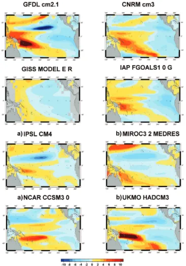
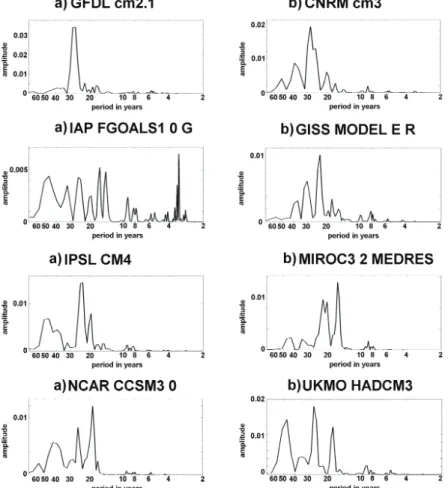
In Fig. 5, are presented the spatial patterns of the first rotated EOF for each CGCM control run and in Fig. 6 the power spectra of their respective PC. Note that, as for the 10

rotated EOF of Fig. 3, the maximum of the PC has been normalised to 1 and we have chosen the same colour scale.

Looking at Fig. 5, we note that all CGCM control runs show spatial patterns with a magnitude comparable to reconstructed (Fig. 3) and observed ones (Fig. 1a). The

magnitudes are between −12 mm yr−1 and +12 mm yr−1. Furthermore 6 models out

15

of 8 (GFDL, CNRM, GISS, IAP, NCAR and UKMO) show a clear east-west dipole in the Tropical Pacific like in observations. But, in general, patterns di_ffer in shape. In 4 models (GFDL, CNRM, NCAR and UKMO), patterns are fairly similar with each other and exhibit some common features with the observed ones. They are dominated by a strong positive signal south-east of Papua-New Guinea and a more modest posi-20

tive anomaly north of Papua-New Guinea that are seen in the observations as well (see Figs. 1a and 3 for comparison). For the NCAR and the UKMO runs, they ex-tend slightly too far eastward in the Equatorial Pacific. They exhibit as well a negative trend anomaly east of the Philippines. This one appears also in the observations but is actually opposite in sign.

(15)

CPD

8, 349–389, 2012

Title Page

Tables Figures

◭ ◮

Back Close

Full Screen / Esc

Discussion

P

a

per

|

Dis

cussion

P

a

per

|

Discussion

P

a

per

|

Discussio

n

P

a

per

The power spectra of the first PCs are shown on Fig. 6. Note that the IAP simulation is an exception: it is the only one to show a significant amount of variance of its PC in the inter-annual waveband. Except for this run, all PCs concentrate their variance into a few peaks in the multi-decadal waveband. It indicates that in the CGCM control runs, the Tropical Pacific “17 yr” trends appear to fluctuate with time at multi-decadal 5

time scales like in the observations. The GFDL and CNRM runs present a unique peak centred on 28 yr indicating that their spatial trend patterns fluctuate at time scales of 25–30 yr like in the observations. The GISS, NCAR and UKMO runs show instead three peaks centred at 20 yr, 28 yr and 40 yr (up to 50 yr in the UKMO run).

To investigate this further, we analysed the “17 yr” sea level trends averaged over 10

box A and B for each model. As for the reconstructed sea level, the two time series exhibit a strong anti-correlation (not shown) indicating that in the control runs as well, “17 yr” sea level trends in the Tropical Pacific behave as a dipole. Furthermore, the box B signal correlates well with the NINO3 index smoothed with a 10 yr running mean: the

correlation coefficients are between 0.58 (for the CNRM cm3 control run) and 0.82 (for

15

the IAP fgoals 1.0 control run) (SL of 99 %).

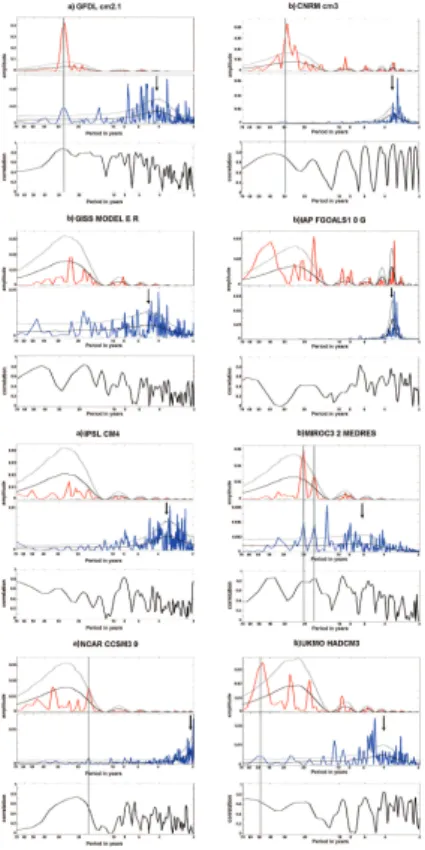
We computed the power spectra of the NINO3 index and the box B “17 yr” sea level trends of each model control run (see Fig. 7). The long time period covered by the control runs allows capturing the multi-decadal variability of both signals that could not be reached with the shorter length of both reconstruction and observations.

20

NINO3 indices of the control runs are shown in Fig. 7 together with their respective autoregressive (AR2) null hypothesis and 95 % confidence interval. The AR2 random processes have been chosen using the same procedure as described in Sect. 4.1. As for the observations, AR2 processes appear to fit properly the NINO3 index spectra. It indicates that for each CGCM control run also, the linear damped oscillator models 25

(16)

CPD

8, 349–389, 2012

Title Page

Tables Figures

◭ ◮

Back Close

Full Screen / Esc

Discussion

P

a

per

|

Dis

cussion

P

a

per

|

Discussion

P

a

per

|

Discussio

n

P

a

per

|

and a fairly good distribution of their variance between inter-annual and multi-decadal time scales. The GISS run shows a too low total variance. The CNRM, IAP, IPSL and NCAR runs have their range of preferred time scales centred around 3 or 2 yr instead of 4 yr, and they show too large variance in the inter-annual timescales compared to the observations. The MIROC run shows too much of its variance in the multi-decadal 5

time scales. It is interesting to note that actually most of the CGCM runs (except the IPSL and the IAP ones) show several peaks significant at the 95 % level of confidence in the multi-decadal waveband. But their central periods di_ffer. In particular, the GFDL, CNRM, GISS, MIROC and UKMO runs agree on the presence of a significant peak at periods around 20–30 yr.

10

Concerning the “17 yr” sea level trends averaged over box B, their spectra are shown on Fig. 7 along with their null hypothesis. The null hypothesis here is the assertion that the “17 yr” box B sea level trends are undistinguishable from the “17 yr” trends of the AR2 process that best fit the sea level in box B. This choice was driven by the same reasons as in Sect. 4.1. We added also the 95 % confidence on Fig. 7.

15

The spectra showed in Fig. 7 are not significant in the inter-annual waveband. At these time scales the power spectra of the “17 yr” trend time series are actually

dom-inated by the auto-correlation coming from the overlapping offthe 17 yr windows. For

the multi-decadal waveband, we note that 6 CGCM runs (GFDL, CNRM, IAP, MIROC, NCAR and UKMO), show some significant peaks at the 95 % confidence level. They 20

confirm that “17 yr” sea level trends oscillate significantly at multi-decadal time scales in the Tropical Pacific. Furthermore, except for the IAP run, each significant peak is asso-ciated with a significant peak of its respective NINO3 index spectrum (see Fig. 7). This indicates that for the majority of the control runs, the significant low frequency fluctua-tion of the “17 yr” sea level trends at multi decadal time scales follows an ENSO-related 25

significant low frequency modulation.

(17)

CPD

8, 349–389, 2012

Title Page

Tables Figures

◭ ◮

Back Close

Full Screen / Esc

Discussion

P

a

per

|

Dis

cussion

P

a

per

|

Discussion

P

a

per

|

Discussio

n

P

a

per

between 0 and 100 %). In particular, it indicates for each frequency band how much two signals correlate. Figure 7 shows that for 5 models (GFDL, CNRM, MIROC, NCAR and UKMO) the 17 yr signal in box B is very coherent with the NINO3 index at low fre-quency. In particular, at each frequency where a significant peak of both the 17 yr sea level and its respective NINO3 index can be found (see the grey vertical bars in Fig. 7), 5

the coherence between both signals is very high: more than 70 % for the GFDL, CNRM, MIROC and UKMO models and 60 % for the NCAR model. It confirms a fairly strong relationship between both signals at these low frequencies, as could be expected in the Tropical Pacific region.

Finally, in general, CGCM control runs show results fairly similar to what was sug-10

gested by the reconstructed and the observed ones. Indeed, the Tropical Pacific trends computed over successive “17 yr” windows also show significant low-frequency mod-ulations in 6 out of 8 CGCM control runs. In 5 of them, the fluctuations appear to be tightly linked to significant ENSO low frequency modulation. Furthermore, 4 of these models (GFDL, CNRM, NCAR and UKMO) exhibit almost the same “17 yr” spatial trend 15

patterns and they display common feature with the reconstructed and the observed ones.

There are still some discrepancies between the CGCMs control runs and the recon-struction or the observations. The spatial trend patterns of the first rotated EOF of the

GFDL, CNRM, NCAR and UKMO control runs differ from the reconstructed and the

20

observed ones north of 5◦

N (Fig. 3). The power spectra of the observed NINO3 index

and their NINO3 index (compare Fig. 4c and Fig. 7) differ as well. The observed NINO3

index does not show any significant multi-decadal variability at time scales superior to 15 yr while the NINO3 indices from control runs do. But actually these discrepancies with the observations are not necessarily significant because the time period covered 25

(18)

CPD

8, 349–389, 2012

Title Page

Tables Figures

◭ ◮

Back Close

Full Screen / Esc

Discussion

P

a

per

|

Dis

cussion

P

a

per

|

Discussion

P

a

per

|

Discussio

n

P

a

per

|

missed by the shorter observation datasets. We verified this point on the GFDL control run. We split the 500 yr GFDL control run into 8 independent 60 yr long samples (the time length covered by the reconstruction). For each of them we computed the first rotated EOF from the “17 yr” trend maps as done for the reconstruction in Sect. 4.1. Among the 8 resulting rotated EOFs, 6 were very similar to the rotated EOF computed 5

over the whole control run time span (Fig. 5) and 2 turned out to be very similar to the observed one (Fig. 3). In Fig. 8 we present one of them: the first rotated EOF com-puted from the 4th sample (years 220 to 280) of the GFDL control run. It explains 49 % of the total variance. To be fully consistent with the observations, Fig. 8 also shows the power spectrum of the NINO3 index computed over a 155 yr time period, i.e. the 10

time period covered by the NINO3 index (it has been computed on the years 125–280 of the GFDL control run). Comparing Figs. 8 and 3, the model strikingly resembles the observations on the 4th sample case. The spatial patterns of the first rotated EOF are very close to the observed ones and the PC follows as well the NINO3 index with a quasi periodicity of between 20–30 yr. It is interesting to note that even the power 15

spectrum of the NINO3 index is in better agreement with the data: the multi-decadal peak observed in Fig. 7 around 28 yr is not significant anymore. As for the observa-tions (Fig. 4c) the NINO3 power spectrum does not show any multi-decadal variability at periods superior to 15 yr. It indicates that a “17 yr” sea level trend variability similar to the reconstructed one can be found among the 60 year long samples of a control 20

run.

4.2.2 20cm3 runs

In this section we consider the CGCMs 20th century runs (20c3m) to check whether

any di_fferences with the control runs can be found or not. Our approach is to consider

that the best estimation of the internal modes of variability of the climate system are 25

(19)

CPD

8, 349–389, 2012

Title Page

Tables Figures

◭ ◮

Back Close

Full Screen / Esc

Discussion

P

a

per

|

Dis

cussion

P

a

per

|

Discussion

P

a

per

|

Discussio

n

P

a

per

forcing. Hence they provide an estimation of the modes of variability of a preindustrial, unperturbed, steady climate. The point is to see whether 20th century runs makes

any significant differences with respect to a steady state climate in terms of “17 yr”

sea level trends (the null hypotheses here is the assertion that the 20th century runs are undistinguishable from control runs in terms of “17 yr” sea level trend patterns and 5

variability).

As in the previous analysis, we computed for each CGCM 20c3m run sea level trend maps over successive “17 yr” windows and we performed two comparisons with the control runs: one with the “17 yr” spatial trend patterns and one with the “17 yr” aver-aged trend over box B.

10

For the first comparison, we considered the “17 yr” spatial trend patterns of the ro-tated EOF of the control runs as the reference. Then we projected the set of “17 yr” trend maps computed from each 20c3m run outputs on these patterns (each 20c3m run outputs was projected on its respective control run spatial patterns). The resulting PCs show how the reference spatial patterns from the control runs fluctuate through 15

the simulated 20th century climates. Their power spectra are plotted in Fig. 9. When several 20c3m runs were available for a given model, each PC was also plotted on the same graph. We added as well the power spectra of the control run leading PC (previously presented in Fig. 7). But here, for a consistent comparison with the 20c3m power spectra, they were computed over subsets of 140 yr (length of the 20c3m runs) 20

instead of the whole multi-centennial control run. We used a chunk spectral estimator (see von Storch and Zwiers, 1999) to compute them. This method consists in dividing the time series into a number of chunks of equal length and to estimate the spectrum by averaging the spectra obtained over each subset. It allows also estimating the 95 % confidence level. We added them on Fig. 9. But, note that here, only very few inde-25

(20)

CPD

8, 349–389, 2012

Title Page

Tables Figures

◭ ◮

Back Close

Full Screen / Esc

Discussion

P

a

per

|

Dis

cussion

P

a

per

|

Discussion

P

a

per

|

Discussio

n

P

a

per

|

It is interesting to note that in Fig. 9 all CGCM 20c3m runs show some low frequency modulation of the spatial patterns like in the reconstruction and the control runs. Among models with complete external forcing (i.e. anthropogenic green house gas emissions plus solar and volcanic variability, see Sect. 3.3 and Table 1), only 1 model out of 6

(GISS) shows significant differences in the leading PC between its control run and its

5

20c3m run. 3 models (GFDL, MIROC and NCAR) show instead differences that are not

significant. The 2 models left (CNRM and UKMO) actually show differences that reach

the 95 % confidence level. But these 2 models only have 350 yr of control run. This enabled us to compute only 2 chunks to deduce the 95 % confidence level which makes their estimation particularly unreliable. So we assume actually that, for these 2 models, 10

the di_fferences are not significant. Concerning the IPSL model, which only takes into

account the anthropogenic external forcing (see Sect. 3.3 and Table 1), significant

differences can be seen in the leading PC between the control run and the 20c3m run.

But for the IAP model which includes the anthropogenic forcing and solar variability (but

no forcing due to volcanic eruptions), no significant differences are observed. Finally

15

there is a majority of models (6 out of 8) which do not show significant difference in

“17 yr” sea level trend patterns between their control run and their 20th century runs. In particular, 5 out of the 6 models which include complete external forcings do not show significant differences.

In the second comparison, we have considered the “17 yr” sea level trend averaged 20

over box B in the 20c3m runs. Their power spectra are plotted in Fig. 10 along with the power spectra of the “17 yr” averaged trend in box B computed from the control runs. As for the PCs, these power spectra are the power spectra already presented on Fig. 6 except that they were computed over subsets of 140 yr to be consistent with the 20c3m power spectra. We used as well a chunk spectral estimator to do so. As for the PCs, 25

(21)

CPD

8, 349–389, 2012

Title Page

Tables Figures

◭ ◮

Back Close

Full Screen / Esc

Discussion

P

a

per

|

Dis

cussion

P

a

per

|

Discussion

P

a

per

|

Discussio

n

P

a

per

more reliable estimations of the confidence intervals. The AR2 process power spectra and their 95 % confidence level are plotted in Fig. 10. Among models with complete

external forcing, 2 models out of 6 (CNRM and UKMO) show a significant difference

between the power spectra computed from their control run and their 20c3m run. 3

models (GFDL, GISS and NCAR) show both some 20c3m runs that di_ffer significantly

5

from their control run and some which do not. For each of these 3 models, only one run among all available 20c3m runs shows significant differences (i.e. 1 out of 4 available for the GFDL model, 1 out of 8 for the GISS model and 1 out of 2 for the NCAR model).

Finally 1 model (MIROC) do not show any significant differences between its 20c3m

run and its control run. 10

In this comparison the IPSL model, (with anthropogenic forcing only), does not show

significant differences between its control run and its 20c3m run while the IAP model

(whose 20c3m run contain green house gas emissions and solar variability) shows some. Finally, among the nineteen 20c3m runs available from our dataset (see Ta-ble 1), 13 of them do not show any significant differences with their respective control 15

runs (this ratio increases to 12 out of 17 when considering only 20c3m runs with

com-plete external forcing). Only 6 20c3m runs show some differences. In total, only 5

20c3m runs show differences if we consider only those with complete external forcing.

Nevertheless it is interesting to note that for each of these 5 runs, the power spectra reveal that the “17 yr” trends fluctuations in the 20c3m runs present a peak at higher 20

frequency with more variance than in their respective control run.

5 Summary and discussion

Previous studies have shown that the sea level trend patterns observed in the Tropi-cal Pacific through 17 yr long precise altimetry observations (1993–2009) are largely of thermal origin, (Ishii and Kimoto, 2009; Levitus, 2005; Levitus et al., 2009; Lom-25

(22)

CPD

8, 349–389, 2012

Title Page

Tables Figures

◭ ◮

Back Close

Full Screen / Esc

Discussion

P

a

per

|

Dis

cussion

P

a

per

|

Discussion

P

a

per

|

Discussio

n

P

a

per

|

2010). In this region, observed and thermosteric sea level trends are tightly linked to the ENSO modes of variability known to occur on a broad range of time scales, from inter-annual to multi-decadal (Knutson and Manabe, 1998; Lau and Weng, 1999; Vi-mont et al., 2002; ViVi-mont, 2005). So the “17 yr” trends observed by satellite altimetry in the Tropical Pacific are expected to fluctuate on these time scales. The results pre-5

sented in Sect. 4.1 confirm that this is indeed the case. On the basis of a past sea level reconstruction (1950–2009), we find that the Tropical Pacific trend patterns over suc-cessive 17 yr windows fluctuate in time and show some periods during which sea level rise accelerates or decelerates (or equivalently trend patterns of increasing or decreas-ing intensity). The trend patterns behave as a fluctuatdecreas-ing east-west dipole, followdecreas-ing 10

a low-frequency modulation of ENSO. The relatively short time span of the 60 yr long reconstruction makes it difficult to precisely determine the characteristic time-scales of the patterns fluctuation but some value around 25 yr is suggested by the observations. CGCM control runs with constant, preindustrial external forcing, show fairly similar results. Indeed, 4 out of 8 CGCM control runs (GFDL, CNRM, NCAR and UKMO) 15

show significant “17 yr” sea level trend fluctuations tightly linked to significant ENSO low-frequency modulations as well. They display the same “17 yr” spatial trend

pat-terns which differ slightly from the reconstructed ones. But it has been showed for the

GFDL control run that this is probably due to the different time period covered by the

reconstruction and the control runs. So, the internal variability of the climate system, 20

simulated here by the CGCM control runs, seems to be well able to explain most of the sea level trend pattern fluctuations of the Tropical Pacific seen in the reconstruction and observed by altimetry. Note nevertheless that the different control runs do not al-ways agree on the characteristic periods of these fluctuations. The GFDL and CNRM control runs exhibit periodicities in the range 25–33 yr close to what is suggested by 25

(23)

CPD

8, 349–389, 2012

Title Page

Tables Figures

◭ ◮

Back Close

Full Screen / Esc

Discussion

P

a

per

|

Dis

cussion

P

a

per

|

Discussion

P

a

per

|

Discussio

n

P

a

per

The CGCM 20th century runs with external forcing (including anthropogenic forcing) show similar sea level trend behaviours for the Tropical Pacific as in the control runs. Actually, a majority of the 20c3m runs which include a complete external forcing (12 out of 17) do not show any significant differences with their respective control run either in terms of temporal or spatial structures. Consequently, because the 20c3m and con-5

trol runs provide similar results, we conclude that the natural variability of the climate system is still the dominant contributor to the fluctuations of the “17 yr” spatial trend patterns in the Tropical Pacific, as the present analysis does not detect any clear effect of the external forcing whether of anthropogenic origin or of natural origin (solar and volcanic variability). In other words, over the short altimetry record (17 yr), the ampli-10

tude of the noise represented here by the natural climate variability is so strong in the Tropical Pacific that it prevents us from detecting the signal of the anthropogenic forcing on the regional variability of the sea level trends in this region.

Nevertheless a minority of 20th century runs (see Sect. 4.2) seem to suggest that the impact of the external forcing could be possibly seen in the characteristic frequency 15

band of the 17 yr trend patterns oscillation. Several 20th century runs indeed show higher frequency oscillations for the 17 yr trend patterns than their respective control run (as explained earlier). But this remains very unclear. To get a clearer picture, we would need both more 20th century runs (to perform statistics on how many runs support this assertion) and longer runs with external forcing to compute more accurate 20

power spectra. These runs should be available within the CMIP5 project. This will be the subject of future investigations.

Acknowledgements. M. Becker is supported by an ANR CNRS grant number ANR-09-CEP-001-01 (CECILE project). W. Llovel is supported by a NASA Postdoctorate fellowship.

(24)

CPD

8, 349–389, 2012

Title Page

Tables Figures

◭ ◮

Back Close

Full Screen / Esc

Discussion

P

a

per

|

Dis

cussion

P

a

per

|

Discussion

P

a

per

|

Discussio

n

P

a

per

|

The publication of this article is financed by CNRS-INSU.

References

Ablain, M., Cazenave, A., Valladeau, G., and Guinehut, S.: A new assessment of the error budget of global mean sea level rate estimated by satellite altimetry over 1993–2008, Ocean

5

Sci., 5, 193–201, doi:10.5194/os-5-193-2009, 2009.

Becker, M., Meyssignac, B., Llovel, W., Cazenave, A., and Delcroix, T.: Sea level vari-ations at Tropical Pacific Islands since 1950, Global Planet. Change, 81–82, 85–98, doi:10.1016/j.gloplacha.2011.09.004, 2012.

Bindoff, N. L., Willebrand, J., Artale, V., Cazenave, A., Gregory, J., Gulev, S., Hanawa, K., Le

10

Qu ´er ´e, C., Levitus, S., Nojiri, Y., Shum, C. K., Talley, L. D., and Unnikrishnan, A.: Obser-vations: oceanic climate change and sea level, in: Climate Change 2007: The Physical Science Basis. Contribution of Working Group I to the Fourth Assessment Report of the In-tergovernmental Panel on Climate Change, edited by: Solomon, S., Qin, D., Manning, M., Chen, Z., Marquis, M., Averyt, K. B., Tignor, M., and Miller, H. L., Cambridge University

15

Press, Cambridge, UK and New York, NY, USA, 2007.

Brigham, E. O.: The Fast Fourier Transform, Prentice-Hall, Englewood Cliffs, 1974.

Brodeau, L., Barnier, B., Treguier, A., Penduff, T., and Gulev, S.: An ERA40-based atmospheric forcing for global ocean circulation models, Ocean Model., 31, 88–104, 2010.

Carrere, L. and Lyard, F.: Modeling the barotropic response of the global ocean to atmospheric

20

wind and pressure forcing – comparisons with observations, Geophys. Res. Lett., 30, 1275– 1279, 2003.

(25)

CPD

8, 349–389, 2012

Title Page

Tables Figures

◭ ◮

Back Close

Full Screen / Esc

Discussion

P

a

per

|

Dis

cussion

P

a

per

|

Discussion

P

a

per

|

Discussio

n

P

a

per

Carton, J., Giese, B., and Grodsky, S.: Sea level rise and the warming of the oceans in the Simple Ocean Data Assimilation (SODA) ocean reanalysis, J. Geophys. Res.-Oceans, 110, C09006, doi:10.1029/2004JC002817, 2005.

Cazenave, A. and Llovel, W.: Contemporary sea level rise, Annu. Rev. Mar. Sci., 2, 145–173, 2010.

5

Cazenave, A. and Nerem, R.: Present-day sea level change: observations and causes, Rev. Geophys., 42, RG3001, doi:10.1029/2002GL016473, 2004.

Christiansen, B., Schmith, T., and Thejll, P.: A surrogate ensemble study of sea level recon-structions, J. Climate, 23, 4306–4326, 2010.

Church, J. A., White, N. J., Coleman, R., Lambeck, K., and Mitrovica, J. X.: Estimates of the

10

regional distribution of sea level rise over the 1950–2000 period, J. Climate, 17, 2609–2625, 2004.

Collins, W. D., Rasch, P. J., Boville, B. A., Hack, J. J., McCaa, J. R., Williamson, D. L., Kiehl, J. T., Briegleb, B., Bitz, C., Lin, S. J., Zhang, M., and Dai, Y.: Description of the NCAR Community Atmosphere Model (CAM3.0), Technical Note TN-464+STR, National Center

15

for Atmospheric Research, Boulder, 2004.

Delworth, T., Broccoli, A., Rosati, A., Stouffer, R., Balaji, V., Beesley, J., Cooke, W., Dixon, K., Dunne, J., Dunne, K., Durachta, J., Findell, K., Ginoux, P., Gnanadesikan, A., Gordon, C., Griffies, S., Gudgel, R., Harrison, M., Held, I., Hemler, R., Horowitz, L., Klein, S., Knutson, T., Kushner, P., Langenhorst, A., Lee, H., Lin, S., Lu, J., Malyshev, S., Milly, P., Ramaswamy, V.,

20

Russell, J., Schwarzkopf, M., Shevliakova, E., Sirutis, J., Spelman, M., Stern, W., Winton, M., Wittenberg, A., Wyman, B., Zeng, F., and Zhang, R.: GFDL’s CM2 global coupled climate models, Part, I.: Formulation and simulation characteristics, J. Climate, 19, 643–674, 2006. D ´equ ´e, M., Dreveton, C., Braun, A., and Cariolle, D.: The ARPEGE/IFS atmosphere model –

a contribution to the french community climate modeling, Clim. Dynam., 10, 249–266, 1994.

25

Di Lorenzo, E., Cobb, K. M., Furtado, J. C., Schneider, N., Anderson, B. T., Bracco, A., Alexan-der, M. A., and Vimont, D. J.: Central Pacific El Nino and decadal climate change in the North Pacific Ocean, Nat. Geosci., 3, 762–765, 2010.

Gnanadesikan, A., Dixon, K., Gri_ffies, S., Balaji, V., Barreiro, M., Beesley, J., Cooke, W., Delworth, T., Gerdes, R., Harrison, M., Held, I., Hurlin, W., Lee, H., Liang, Z., Nong, G.,

30

(26)

CPD

8, 349–389, 2012

Title Page

Tables Figures

◭ ◮

Back Close

Full Screen / Esc

Discussion

P

a

per

|

Dis

cussion

P

a

per

|

Discussion

P

a

per

|

Discussio

n

P

a

per

|

J. Climate, 19, 675–697, 2006.

Gomez, N., Mitrovica, J., Tamisiea, M., and Clark, P.: A new projection of sea level change in response to collapse of marine sectors of the Antarctic Ice Sheet, Geophys. J. Int., 180, 623–634, 2010.

Gordon, C., Cooper, C., Senior, C. A., Banks, H., Gregory, J. M., Johns, T. C., Mitchell, J. F.

5

B., and Wood, R. A.: The simulation of, SST, sea ice extents and ocean heat transports in a version of the Hadley Centre coupled model without flux adjustments, Clim. Dynam., 16, 147–168, 2000.

Greatbatch, R.: A note on the representation of steric sea-level in models that conserve volume rather than mass, J. Geophys. Res.-Oceans, 99, 12767–12771, 1994.

10

Hourdin, F., Musat, I., Bony, S., Braconnot, P., Codron, F., Dufresne, J. L., Fairhead, L., Filiberti, M. A., Friedlingstein, P., Grandpeix, J. Y., Krinner, G., Levan, P., Li, Z. X., and Lott, F.: The LMDZ4 general circulation model: climate performance and sensitivity to parameterized physics with emphasis on tropical convection, Clim. Dynam., 27, 787–813, 2006.

Ishii, M. and Kimoto, M.: Reevaluation of historical ocean heat content variations with

time-15

varying XBT and MBT depth bias corrections, J. Oceanogr., 65, 287–299, 2009.

Jin, X. Z., Zhang, X. H., and Zhou, T. J.: Fundamental framework and experiments of the third generation of the IAP/LASG world ocean general circulation, Adv. Atmos. Sci., 16, 197–215, 1999.

Johns, T. C., Durman, C. F., Banks, H. T., Roberts, M. J., McLaren, A. J., Ridley, J. K., Senior,

20

C. A., Williams, K. D., Jones, A., Rickard, G. J., Cusack, S. Ingram, W. J., Crucifix, M., Sexton, D. M. H., Joshi, M. M., Dong, B. W., Spencer, H., Hill, R. S. R., Gregory, J. M., Keen, A. B., Pardaens, A. K., Lowe, J. A., Bodas-Salcedo, A., Stark, S., and Searl, Y.: The new Hadley Centre climate model HadGEM1: evaluation of coupled simulations, J. Climate, 19, 327–1353, 2006.

25

K-1 Model Developers: K-1 Coupled Model (MIROC) Description, K-1 Technical Report 1, Center for Climate System Research, University of Tokyo, 2004.

Kaplan, A., Cane, M., Kushnir, Y., Clement, A., Blumenthal, M., and Rajagopalan, B.: Analy-ses of global sea surface temperature 1856–1991, J. Geophys. Res.-Oceans, 103, 18567– 18589, 1998.

30

(27)

CPD

8, 349–389, 2012

Title Page

Tables Figures

◭ ◮

Back Close

Full Screen / Esc

Discussion

P

a

per

|

Dis

cussion

P

a

per

|

Discussion

P

a

per

|

Discussio

n

P

a

per

Knutson, T. and Manabe, S.: Model assessment of decadal variability and trends in the Tropical Pacific Ocean, J. Climate, 11, 2273–2296, 1998.

Kohl, A. and Stammer, D.: Decadal sea level changes in the 50-year GECCO ocean synthesis, J. Climate, 21, 1876–1890, 2008.

Large, W. and Yeager, S.: Diurnal to decadal global forcing for ocean and sea-ice models: the

5

datasets and flux climatologies, NCAR technical note: NCAR/TN460+STR, CGD Division of the National Center for Atmospheric Research, available on the GFDL CORE web site, 2004.

Lau, K. and Weng, H.: Interannual, decadal-interdecadal, and global warming signals in sea surface temperature during 1955–97, J. Climate, 12, 1257–1267, 1999.

10

Le Traon, P., Nadal, F., and Ducet, N.: An improved mapping method of multisatellite altimeter data, J. Atmos. Ocean. Tech., 15, 522–534, 1998.

Le Traon, P. L. and Ogor, F.: ERS-1/2 orbit improvement using TOPEX/POSEIDON: the 2 cm challenge, J. Geophys. Res., 103, 8045–8057, 1998.

Levitus, S.: Warming of the world ocean, 1955–2003, Geophys. Res. Lett., 32, L02604,

15

doi:10.1029/2004GL021592, 2005.

Levitus, S., Antonov, J. I., Boyer, T. P., Locarnini, R. A., Garcia, H. E., and Mishonov, A. V.: Global ocean heat content 1955–2008 in light of recently revealed instrumentation problems, Geophys. Res. Lett., 36, L07608, doi:10.1029/2008GL037155, 2009.

Liu, H. L., Zhang, X. H., Li, W., Yu, Y. Q., and Yu, R. C.: An eddy-permitting oceanic general

20

circulation model and its preliminary evaluations, Adv. Atmos. Sci., 21, 675–690, 2004. Llovel, W., Cazenave, A., Rogel, P., Lombard, A., and Nguyen, M. B.: Two-dimensional

re-construction of past sea level (1950–2003) from tide gauge data and an Ocean General Circulation Model, Clim. Past, 5, 217–227, doi:10.5194/cp-5-217-2009, 2009.

Lombard, A., Cazenave, A., DoMinh, K., Cabanes, C., and Nerem, R.: Thermosteric sea level

25

rise for the past 50 years; comparison with tide gauges and inference on water mass contri-bution, Global Planet. Change, 48, 303–312, 2005a.

Lombard, A., Cazenave, A., Le Traon, P., and Ishii, M.: Contribution of thermal expansion to present-day sea-level change revisited, Global Planet. Change, 47, 1–16, 2005b.

Lombard, A., Garric, G., and Penduff, T.: Regional patterns of observed sea level change:

30