Abstract
Instability of liquefaction is one of the major reasons which results in the failure of earth structure such as dam. The present study focuses on the simulation of static liquefaction behavior for granular materials such as sand and sand-silt mixtures. Based on microme-chanical analysis of inter-particle behavior, a simple one-scale model is proposed to simulate the stress-strain response of sand; then the proposed model is extended to simulate the sand-silt mixtures using the mixture theory combining the properties of sand and silt accord-ing to their proportions. Empirical expressions are introduced to fit the critical state strength and the location of the critical state line for each mixture. Parameters of the model can be divided into two categories: the first seven parameters have the same values either with pure sand or pure silt for silt-sand with any given fines con-tent; the other three parameters are the function of fines content and three more parameters are required to estimate their values. The predicted results of triaxial test of sand and sand-silt mixtures with different fine content, which has a good agreement with the results of laboratory tests, suggest that the proposed model can simulate static liquefaction behavior of sand and sand-silt mixtures.
Keywords
Constitutive model, granular materials, sand-silt mixtures
A Simple One-Scale Constitutive Model
for Static Liquefaction of Sand-Silt Mixtures
1 INTRODUCTION
Instability of liquefaction is one of the major reasons which results in the failure of earth structures such as dam. “Liquefaction” is used for the first time by Hazen (1920), describing the failure of the Calaveras dam’s failure. Terzaghi (1925) defined the essential processes of liquefaction and the sub-sequent description by Casagrande’s (1936, 1965) together formed the basis for research of liquefac-tion at that time. Casagrande defined the critical void ratio (CVR) concept in his early paper. Seed and Lee (1966) took the pore pressure value as the basis for analysis of sand liquefaction, proposing the concept of “initial liquefaction”. Casagrande and Castro (1975) refined the definition of critical
Yang Liu a, * C S Chang b Shun-Chuan Wu a, *
a Department of Civil Engineering,
Uni-versity of Science and Technology, Bei-jing, 100083, China
b Department of Civil and
Environmen-tal Engineering, University of Massachu-setts, Amherst, MA 01003, U.S.A
* Corresponding author:
[email protected] [email protected]
http://dx.doi.org/10.1590/1679-78251901
void ratio and proposed the concept “steady state strength”, which is used to estimate sand liquefac-tion failure. Later several concepts such as “steady state deformaliquefac-tion”, “steady state line”, “flow structure” were proposed to describe the liquefied deformation mechanism of saturated granular mixture by several researchers (Poulos,1981,1985; Castro,1992; Ishihara,1993; Bazier and Do-bry,1995) .
The concept of liquefaction covers the static liquefaction caused by static loading and the cyclic liquefaction resulted from mechanical vibration such as earthquake, explosion and dynamic loading. Conceptually, when the deviatoric stress-strain curve appears obvious strain-softening phenomenon during monotonic loading and the deviatoric stress falls to zero after the peak value, the character-istics of saturated granular mixture appears like fluid, which is defined as “static liquefaction”. This kind of liquefaction occurs without dynamic load, and is defined as static liquefaction distinguished from the liquefaction caused by vibration.
Many research works has been carried on the cyclic liquefaction (Seed etc. 1966; Ishihara, 1975, 1993; Zienkiewicz etc.1984; Zhou, 1995; Zhang etc. 2006; James etc 2011). In recent years, more and more researchers realized the severity of the failure caused by static liquefaction, beginning to study the static liquefaction characteristics of grain material (Verdugo,1996; Yamamuro,1998; Boukpeti, 2000; Mroz, 2003; Lade, 2011) and stability of earth structure (Fourier, 2001; Anderson, 2012; Bedin, 2012).
One important aspect of liquefaction study is to predict the stress-strain relationship of granular materials that is susceptible to liquefaction. The models for stress-strain behavior of granular mate-rials (for example sand or sand-silt mixtures) can be generally categorized into two approaches: the conventional plasticity approach and the micromechanics based approach. The stress-strain models based on traditional plasticity is a one-scale approach, which can be found in the works of many researchers (Desai and Siriwardane, 1984; Wood, 1990; Prevost, 1985; Dafalias and Herrmann, 1982; Klisinski, 1988; Mroz, 2003).
The stress-strain models based on micromechanics approach is a multi-scale approach. The mi-cromechanics models provide a set of constitutive laws for the behavior at local scale (i.e. the inter-particle level). The stress-strain behavior is then obtained through an integration process. Many micromechanics approaches have been proposed to establish elastic (Jenkins ,1988; Walton, 1987; Rothenburg and Selvadurai ,1981; Chang, 1988, 1989; Cambou, and Dubujet, 1995; Emeriault and Cambou ,1996; Liao et al. , 2000; Kruyt and Rothenburg , 2002; Tran et al. ,2012; ) and elasto-plastic constitutive model (Jenkins and Strack,1993; Matsuoka and Takeda ,1980; Chang and Hicher ,2005; Nicot and Darve,2007; Maleej et al. ,2009; Misra and Yang , 2010; Zhu et al., 2010; Zhang and Zhao ,2011; Daouadji and Hicher, et,al, 2013; Misra and Singh ,2014).
Usually, the multi-scale model is more complex than the conventional one-scale model. The added complexity improves the realism of the model in some degree, however, this complexity also make it not easy to be used in real boundary value problem. A practical constitutive model is not only reason-able for describing the static liquefaction behavior of granular materials, but also should intend to be in a simple form with fewer parameters easy to be determined. Along this line, the present study is aimed to develop a simple but effective one-scale constitutive model based on some micromechanical analysis, to simulate the static liquefaction behavior of granular materials such as sand.
envi-environment. It is well know that fines content has a significant influence on the microstructure and behavior of soil. Terzaghi (1956) found the presence of fine particles increase the possibility of form-ing metastable structures. The grain-to-grain fabric of the sandy silt is responsible for their noplastic and noncohensive characteristics, which exert a considerable influence and make them susceptible to liquefaction. Consideration of this natural trend and questions regarding silt influence on engineer-ing behavior of sandy soils has triggered the research on silty sands in recent years. Many investiga-tors (Kuerbis et al. ,1998; Pitmanet al.,1994; Lade and Yamamuro,1997; Thevanayagam, 1998; Thevanayagam and Mohan ,2000; Salgado et al.,2000; Thevanayagam et al. ,2002; Ni et al., 2004; Murthy et al., 2007; Monkul, et al., 2011; and Dash, et al, 2011) have conducted experiment on sand with amount of silt and studied their the stress–strain behavior.
So it is important to consider the effect of fine content on the liquefaction of sand. In this study we adopt a simple but effective way to study this effect: the behavior of silt-sand mixtures is mod-eled using a sort of mixture theory combining the properties of the two soils according to their pro-portions. In particular, empirical expressions are introduced to fit the critical state strength and the location of the critical state line for each mixture.
In the following sections, we firstly introduce a simple one-scale model based on micromechani-cal analysis of inter-particle behavior. Then we extend the model to model sand-silt mixtures using mixture theory. Finally the predicted results from the proposed model are compared with three sets of data of sand and sand-silt mixtures to evaluate its performances in simulating stress-strain rela-tionship of granular materials.
2 A SIMPLE ONE-SCALE MODEL FOR STATIC LIQUEFACTION OF GRANUALAR MATERIALS In this section, based on micromechanical analysis of inter-particle behavior, a simple one-scale model for static liquefaction of sand is proposed. The general numerical results are presented and the response envelope and two-order work predicted from the proposed model is also discussed in simulating the liquefaction instability phenomenon of sand.
2.1 Inter-Particle Behavior of Granule
In granular assembly, particles contact each other; the orientation of a contact plane between two particles is defined by the vector perpendicular to this plane. On each contact plane, an auxiliary local coordinate can be established as shown in Fig. 1.
The contact stiffness of a contact plane includes normal stiffness, kn
, and shear stiffness,
r k. The elastic stiffness tensor is defined by,
e i ij j
f k (1)
( )
e
ij n i j r i j i j
k k n n k s s t t (2)
Where, n, s, t are three orthogonal unit vectors that form the local coordinate system. In general,
n
k and kr
is the normal and tangential elastic stiffness on contact plane, which is supposed to
follow a revised Hertz-Mindlin’s contact law (Chang et al., 1989):
0 2 ; 0 2
n n
n n
n n r n
g g
f f
k k k k
G l G l
(3)
Where, fn is the contact force in normal direction, and Gg is the elastic modulus of ideal grains. l is the branch length connecting the neighboring two particles. Three material constantskn0
,, and
n are needed as input.
The movements of particles at contact plane often result in a dilation/contraction behavior, can be expressed as follows:
0 tan p n r p n r f d f (4)
Where d is the dilatancy parameter. fr is the contact force in tangent direction. The value of
0 in Eq. 4 is assumed to be equal to the critical state friction angle (i.e.
0 cs).A Mohr-Coulomb type yield function, defined in a contact-force space, is assumed to be as fol-lows,
, ,
p 0n r r n r
F f f f f (5)
Where fr
is the resultant shear force and P r
is the resultant plastic sliding. ( )P r
is a hardening function defined by a hyperbolic curve in p
r
plane (Chang and Hicher, 2005). Two material parameters, p and 0
p r
k , are involved in the hardening function:
00 tan tan
p p
r p r p
r p p
n p r r
k
f k
(6)
Where, p0 r
k is related to the normal stiffness kn by a constantp:
0 0 2
n
p p p n
r n n
g f
k k k
G l
The initial slope of the hyperbolic curve is p0/
r n
k f and the value of
rp asymptotically ap-proaches the apparent peak inter-particle friction angle (i.e. tanp).2.2 A Simple One-Scale Stress-Strain Model for Granular Materials
Based on the inter-particle behavior described above, a two-scale micromechanical model may be formed as Chang (Chang, et.al 2005) through an integration process over the behavior for all con-tacts. In the micromechanics approach, the continuum mechanical concept “infinitesimal volume element” (IVE) is treated as a discrete mechanical concept “representative volume element’ (RVE) that embodies an assembly of particle. Then the global stress-train behavior of the representative volume element can be obtained based on the behavior at local scale (i.e. the inter-particle level). However, if we assumed mechanical properties of assembly at all directions are the same as the de-fined plan as described in 2.1., the assembly (global) can be regarded as homogenous materials and the inter-particle behaviors is now defined for a “material point”, which represents an “infinitesimal volume element” of the continuum material. Besides, a density state variable (defined as a function of the critical state void ratio) was introduced for plastic flow, which was postulated to be depend-ent on this variable. In this way, a simple one-scale model can be developed based on inter-particle behaviors.
At the inter-particle (local) level, mechanical variables are contact forces fn , fr and displace-mentsn, r. The constitutive laws, such as yielding function, shear dilation and hardening rules, are defined at the local level using these inter-particle mechanical variables on each contact plane using Eq. (4)- Eq. (7).
At the assembly (global) level, the mechanical variables are stresses p , q and strainsv, r , which can be obtained by integrating the corresponding inter-particle variables (forces fn , fr and displacements n, r) in all orientations under isotropic condition.
Since the overall (global) physical behavior is manifested by the local physical behavior, it seems reasonable to assume that the constitutive laws at the global level takes the same form as those at the local level under the assumption that all. Thus in the one-scale model, the elastic mod-ulus, the yielding function, the shear dilation and the hardening rules can be up scaled by replacing the local variables fn , fr ,
p n
and p
r
by the global variables, p , q, p v
and p r
. The details are given below.
2.2.1 Elastic Behavior
The elastic behavior of the one-scale model can be expressed by the classical elastic theory as fol-lows:
e v
p B (8)
3 e
r
Where, p is the mean stress increment, p(
1 2 3) / 3; e v
is the elastic part of v, v is the volumetric strain increment,v
1 2 3
. q is the shear stress increment (q 3J2 , whereJ2is the second invariant of deviator stress tensor) ; e r
is the elastic part of r , r is the shear strain increment (r 4J2 / 3 , where J2 is second invariant of deviator strain tensor). G is the shear
modulus and B is the bulk modulus, B2 (1G ) / (3(1 2 )) . The Poisson’s ratio
is a constant.The bulk modulus B is considered to be pressure dependent, expressed as follows:
0 /
n ref
BB p p (10)
WhereB0 and n are two material constants: B0 is the reference bulk modulus, and n is a constant exponent. pref is the reference pressure, which is taken to be 1 atm.
2.2.2 Plastic Behavior
As discussed above, the yielding condition, shear dilation and hardening rules can be described di-rectly in the one-scale model using the macro-mechanical variables, p , q and p
v
, p
r
. So, accord-ing to Eq. (4) ~Eq. (7), the dilatancy equation, the yieldaccord-ing condition and harden rules of the one-scale model can be written as follows,
p v u p r q D M p
(11)
, ,
p 0r r
f p q q p (12)
0
p p
p r p
r p p
p r
G M
pM k
(13)
Where, where Mu is the slope of critical state line in p q space, Mu 6sin
cs/ (3 sin )
cs , D is the dilatancy parameter, Mp6sin /(3 sin )p p . A density state function is used to adjust the apparent Coulomb friction angle to friction angle p as follows:tan tan m cr p cs e e
(14)Where m is a positive parameter,
cs is the critical state friction angle. For dense packing, the peak frictional angle p is greater than critical state friction angle (
cs). When the packing structure dilates, the degree of interlocking and the peak frictional angle are reduced, which results in a strain-softening phenomenon.The critical state void ratio (ecr), which is a function of the mean effective stress of p′ ,
/
Where patm is the atmospheric pressure. Equation 15 involves three material constants: eref(zero
intercept), (CSL slope), and (CSL curvature). The plastic stiffness p
G , similar to the plastic stiffness of a contact plane, is assumed to relate to elastic stiffness of the material. It is now assumed to be related to B by a constant
:
0 /
n p
ref
G BB p p (16)
The initial slope of the hyperbolic curve (Eq. 13) is p /
G p, the value of
rp asymptotically approachesMp.We do not have the explicit form of potential function, but we have the gradients of plasticity potential function derived from dilatancy equation as follows:
2
( )
' ' '
g q M
D
p p p
1 ' g q p (17)
One can see that a non-associative flow rule is adopted in the proposed one-scale model.
2.2.3 Stress and Strain Relationship in p q Space
Based on the classical plastic theory, total strain increments can be divided into two parts, i.e., elastic part and plastic part, as follows:
e p ij ij ij
(18)
The elastic part can be calculated by Eqs. (8) and (9) based on elastic theory, and the plastic part can be calculated based on flow rules of plastic theory,
ij ij g d
(19)
Where g is plastic potential function and d is plastic factor, which can be obtained by con-sistency condition, df 0 . In p q stress space the expression of d can be written as follows:
0 2 ( ) ( ) p p r p r p
k dq dp
d
pD M
(20)
Then the plastic increment strain component p p
d and dqp can be calculated according to
Eq.19, 0 3 2 0 2 2 ( )( ) ( ) ( ) ( ) p p p r
p u p
r p
p p
p p r
p q p
r p
k dq dp
d pM q
p M
k dq dp
d d p M
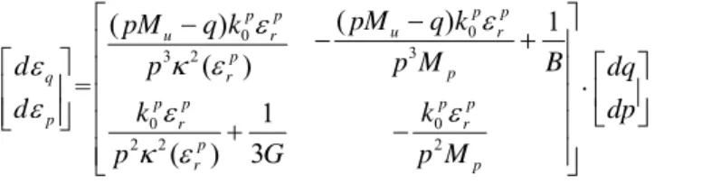
Combining Eq.18, the elasto-plastic stress-strain relationship of the proposed model in p q stress space can be obtained as follows:
0 0
3 3 2
0 0
2 2 2
( ) 1
( )
( ) =
1 ( ) 3
p p p p
u r
u r
p
p r
q
p p p p
p r r
p
r p
pM q k pM q k
p M B
p
d dq
d k k dp
p G p M
(22)
Thus a simple stress-strain relationship for granular materials is established and isotropic hard-ening incorporating one scalar internal variable is adopted in the model. The upscaled response ob-tained from the two-scale micromechanical model(Chang et al, 2005) is kinematic hardening, as the different plastic loading histories on contacts with different orientations are likely to impart a direc-tional character on the macroscopic response of the grain assembly. However, one can see from the predicted response envelope and two-order work that the one-scale model is simple in from but rea-sonable in simulating the liquefaction instability of granular materials. At the same time, no com-plex integrations procedure are needed as micromechanical model does, which is a time consuming process in simulating real boundary problem.
2.2.4 Summary of Parameters of the Proposed Model
Ten model parameters are included in the proposed one-scale model, i.e., the global elastic
0
B ,
and n ; the global plastic constants
,D,m and
cs, critical state constants eref ,,. All parameters are summarized in table.1 and can be determined from stress-strain curves obtained from triaxial tests (see section 3.4).critical state Elas-plastic parameters
elastic plastic
eref
n B0 χ D m0.66 0.016 0.82 0.8 6.3 0.25 8 0.7 4 31
Table 1: Parameters of the proposed one-scale model.
2.2.5 General Numerical Results of the One-Scale Model
(a) Undrained results
(b) Drained results.
Figure 2: General numerical results of the proposed one-scale model.
Numerical results indicate that the proposed model has ability to capture the main features of granular materials behavior. For example, different initial void ratios lead to contracting or dilating behaviors of the sand and deviatoric stress-strain curve appears obvious strain-softening phenome-non during monotonic loading and the deviatoric stress falls to zero after the peak value under un-drained condition. Steady state line (SSL) and instability line (IL) defined for static liquefaction can also be identified on the undrained stress path.
2.2.6 Response Envelope Predicted from the Proposed Model
Response envelope is a useful tool for validating constitutive equations (Doanh, 2000; Kolymbas, 2000; Tamagnini, 2006; Sibille, 2011). The original concept of response-envelopes was presented Lewin & Burland (1970) and Gudehus (1979) in context with the development of constitutive equa-tions. In general, to obtain a response-envelope, a soil element is subjected to a certain stress- or strain-increment. The corresponding “response” of the soil in form of either strain or stress is deter-mined and described graphically. The direction of the applied stress- or strain increment with a constant absolute value is then varied and leads to different stress- or strain responses, endpoints of which are connected to a response envelope.
k
Pa
Axial st ai %
e = .
e = .
e = . e = .
⁑
⁒
⁓
⁔
k
Pa
p' kPa e = .
e = .
e = .
e = .
k
Pa
Axial st ai %
e = .
e = .
e = .
e = .
⁑
⁒
⁓
⁔
‐ ‐ ‐
εv
%
axial st ai %
e = .
e = .
e = .
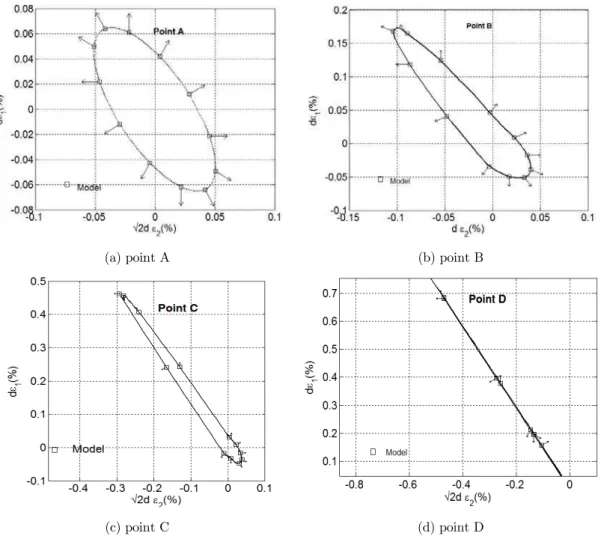
The strain response envelopes predicted from the proposed model was analyzed in the present work. After an initial isotropic compression with confining pressure 200kPa, a drained triaxial load-ing test was simulated in axisymmetric conditions. Stress probe test is performed at 4 stress points, i.e. points A, B, C and D as shown in Fig. 3. Point A (
1 2 3 200kPa, q p/ 0) is an initially isotropic stress state and the other three points are initially anisotropic stress states.( B :1400, = 2003 kPa
,0.75 ; and C:
1480, =200
3 kPa , 0.95 ; and D:1=600, =2003 kPa
, 1.2). Then stress increment dσin all directions with the same norm ( d =10σ kPa) was imposed, and the corresponding strain response dε was computed.Figure 3: Different stress state of stress probe and the location of stress points on stress-strain curve.
The response envelopes predicted from the proposed model are plotted in Fig4. The response envelopes predicted from the model for initially isotropic stress state (point A) is shown in Fig.4 (a). The response envelope is almost identical ellipses centered at the origin of the Rendulic plane of strain increments. The predicted response envelope from point A indicates the response defor-mations at this stress state are mostly elastic.
Figs. 4(b), (c) and (d) are the predicted response envelopes from the proposed model for three anisotropic stress states (i.e., point B, C and D). The patterns of response envelopes for the aniso-tropic stress states are very different from the ellipsis response envelopes for the isoaniso-tropic stress state. The distorted shape of the strain response envelope indicates large plastic strains for some loading direction.
Fig.4(d)shows the strain response envelope for a stress level (
= 1.2) near critical line (orCoulomb friction line
= 1.234). According to the discussions by Darve et. al (2005), near the plas-tic limit condition, the strain response envelope shrinks into a straight line. This straight line indi-cates that, at the plastic limiting condition, the direction of the incremental strain vector is inde-pendent of the direction of the incremental stress vector.k
Pa
Axial st ai %
odel e0=0.75
A B C
(a) point A (b) point B
(c) point C (d) point D
Figure 4: The predicted strain response envelopes from the proposed model at different initially stress state.
2.2.7 Second-Order Work from the Proposed Model
The dot product of the two vectors, dσanddε used in the strain response analysis, represents the second-order work, which is a useful indicator for liquefaction instability of the material. It is of interest to check the possible instabilities due to the stress probes in various directions. For conven-ience, we define a normalized second-order work 2
norm
dW
2 norm
dW = d d
d d
σ ε
σ ε (23)
Thus, 2 norm
dW is equal to the cosine of the angle between the two vectors, dσ and dε. Its value is included in the interval of (-1, 1). Fig. 5 are rose diagrams showing the variation in 2
norm dW with respect to the stress probe direction. In such diagrams, a constant value c = 1 is added to the polar value of 2
norm
dW so that a circle of radius c is drawn in the circular diagrams to represent vanishing values of 2
norm
Fig. 5 shows the rose diagrams for four different levels of shear stress (q/p = 0, 0.75, 0.95, 1,2). The angles shown in Fig. 5 are the stress probing directions (see Fig. 3). Note that the direction of 210 degree is parallel to hydrostatic axis (reduction of mean stress), and the direction of 240 degree is about parallel to Coulomb friction line. Fig. 5 shows that the instabilities occur for probe direc-tions between these two lines.
Figure 5: Results of second-order work from the proposed model for different q/p values.
Material instability is a key to understand the static liquefaction behavior of granular materials such as sand and silty sand (Lade, 1992; Yamamuro and Lade, 1998; .Nicot and Darve, 2006). Ob-viously, the proposed model can capture this kind of instability phenomena and be used to analyze the liquefaction of granular materials.
3 EXTEND THE MODEL TO SIMULATE THE BEHAVIOR OF SAND-SILT MIXTURES
critical state line for each mixture. In this simply way, we extend the proposed model to model liq-uefaction behaviors of sand-silt mixtures.
3.1 Dominant Grains Network in Sand-Silt Mixtures
It is well known that fines content has a significant influence on the microstructure and behavior of soil. Thevanayagam et al. (2002) suggested three kinds of packing structure of mixture depending on the different state of coarse grains and fine grains existed in mixtures. Dominant grains network is the grains network (either coarse grains network or fine grains network) which control the main behavior of the mixtures. Usually, a coarse grains network is formed and controlled the behavior of the mixtures if fine grains in the soil are less than 25%. On the contrary, a fine grains network is formed and controlled the behavior of the mixtures if fine grains in the soil are higher than 35%. For intermediate cases, in which the controlled grains are neither coarse nor fine grain, are not in-cluded in present study.
3.2 Characteristics Change of Sand-Silt Mixtures with Different Fine Content
3.2.1 Void Ratio Characteristics
It is well known that fines content in soil has a considerable control on its packing structure, for that reason, a proper index to connect the pore state of soil should be supposed to take account of both void ratio and the content of fine particles. Such index as inter-granular ratio and inter-fine void ratio are proposed by some researchers (Kuerbis et al., 1989; Mitchell, 1993; Vaid , 1994;Thevanayagam ,1998,2000,2002) for sand-silt mixtures. Chang (2011) suggested a formula to calculate the initial void ratio of soil with fine content less than 25%. According to them, the void ratio of the soil mixtures has been given as:
1
sand c cee f af (24)
For the case of a fine grains skeleton (for example, fc>35%), a similar relationship is proposed
here to calculate the void ratio of the mixtures with fines content greater than 35%:
(1 )
silt c c
ee f b f (25)
Where, esilt is the void ratio of the 100% silt sample. If b=0, Eq. 25 reduces to eesiltfc, which has
the same expression with that for the inter-fine void ratio.(Thevanayagam and Mohan,2000) . If e, esand, and esilt in Eqs. 24 and 25 are replaced by emin, (esand)min, and (esilt)min, the above
expres-sions can also be used to calculate the minimum void ratio of sand-silt mixtures:
min sand min sand min c
e e a e f (26)
min silt min c 1 c
e e f b f (27)
3.2.2 Critical State Void Ratio
The critical void ratio (ecr) described by Eq. 15, i.e. ecr eref
p p'/ atm
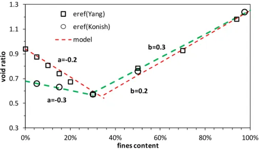
can also be adopted to predict the critical state critical void ratio of the mixtures with different fine content; However, many test results indicates the critical state line is not unique for the mixtures with different fines content(Salgado et al., 2000, Murthy et al., 2007, Fourie and Papageorgiou 2001, Thevanayagam et al. 2002): For the mixtures with low fines contents, the critical state lines have the same slope and curvature but shifting downward as the amount of fines increase; On the other hand, for the mix-tures with high fines contents, the critical state lines shift upward as the amount of fines increase. We chose two sets of test data (Yang, 2004 and Konishi et al., 2007) to study the above trend in sand-silt mixture. The effect of fines content on three parameters eref, , and , were also ana-lyzed. Figure 6 is the critical state data obtained in their tests compared with the predicted results by fitting Eq. 15.
Figure 6: CSLs for different fines contents (Yang, 2004; konish, 2007).
The fitting results are interesting: parameter is found to be almost the same for the whole range of fines content; however, parameter can be regarded as two different values, one for low fines contents (marked in green solid line) and another for high fines contents (marked in red dotted line). Parameter eref varies with the change of fines content, has the same characteristics as that for
void ratio of silt-sand mixtures:
1
ref ref sand c c
e e f af
(for low fines contents) (28)
(1 )ref ref silt c c
e e f b f
(for high fines contents) (29)
. . . . . . . . . .
iti
al
st
at
e
vo
id
a
tio
p' kPa
% % % %
% % % %
% Model
. . . . . . . . . .
iti
al
v
oi
d
at
io
p' kPa
. % . %
. % . %
The predicted results of eref from Eqs. 28 and 29 are given in Fig. 7.
Figure 7: Comparison of the predicted and measured critical state void ratio with different fines content.
3.2.3 Critical State Friction Angle
Many test results indicate that the critical state friction angles
csusually increases with the amount of fine grains in mixture. Murthy et al. (2007) explained these phenomena from the point view of‘flow’ fabric developing at critical state. They believed that the existence of fine particles
wedg-ing between the coarse grains can contribute to the critical strength of soil and thus to the value of critical state friction angle.
From the point view of micromechanics, the critical state friction angles is origin from frictions between particles and the force chain of different packing structures. Mixtures with different fine content have different packing structure and fabric. For mixtures with very low fines contents (for example, lower than 10%), or mixtures with very high fines contents (for example, higher than 70%), the critical state friction angles are experimentally found to be almost not changed with the varia-tion of fine content beyond the threshold content( ie.,10% or 70%). For fines contents between 10%- 70%, Chang and Meidani (2013) proposed a simple model to express the effect of fines content on the critical state friction angles of mixtures as follows:
.
tan tan tan tan
mix
x
cs cs sand cs silt cs silt
c c L
c U c
e
f f
x
f f
(30)
where is a constant needed to input.
fc L and
fc Uare the lower and up limit of fines content.. Typically,
fc L and
fc U can be chosen as 10% and 70% respectively.. . . . . .
% % % % % %
vo
id
a
tio
fi es o te t
e ef Ya g e ef Ko ish
odel
a=‐0.
=0. a=‐0.
3.2.4 Elastic Stiffness of Sand-Silt Mixtures
Reuss (1929) suggested that the average contact stiffness of mixtures can be described as follows:
n1equ
1n sandc
ncsiltf f
k k k
(31)
Where, (kn)equ is the average contact stiffness of the mixtures, (kn)sand is the contact stiffness for
pure sand and (kn)silt is the contact stiffness for pure silt.
Similarly, we assume reference bulk modulus B0 (in Eq.10) is a function of fines content, the follow-ing equation similar to Eq. (31) is chosen to predict the mean bulk modulus of a mixtures com-prised of sand and silt particles,
0
0
01
1 c c
equ sand silt
f f
B B B
(32)
3.3 Extend the One-Scale Model to Simulate Sand-Silt Mixtures
As discussed above, based on mixture theory, the behavior of sand-silt mixtures is dominated by the sand network for low fines content, and by the silt network for high fines content. According to the different dominant grain network, the 10 parameters of the proposed one-scale model can be divided into two categories: the first seven parameters ( i.e., , v, n ,
, D, and m) for sand-silt miture with any given fines content are assumed to be the same values of those for pure sand for sand-silt mixtures with 0% < fc < 25%; and have the same value as those for pure silt forsand-silt mixtures with 35% < fc < 100%. So for sand-silt mixtures with any fine content, these seven
parameters are the same either with pure sand or pure silt.
For the other three parameters (i.e.B0,
csanderef ), we assume bulk modulus B0 , the critical state friction angle cs and reference void ratio eref as a function of fines content. In order to esti-mate the parameters, cs and eref , for sand-silt mixtures, three more parameters a, b and are required. These three additional parameters can be determined by fitting Eqs. (26)- (27) and (30) to triaxial tests data for mixtures with different fines content.In this simple way, we can extend the proposed one-scale model to be suitable for sand-silt mix-tures. Only three more parameters (a, b and) are added to the model.
3.4 Calibration of the Model Parameters
3.4.1 Critical State Parameters
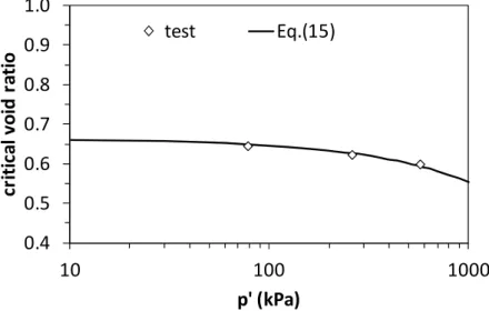
Three critical state parameters, namely,
e
ref (intercept), (CSL slope), and (CSL curvature) are required to define the critical state void ratio. To do so, drained or undrained triaxial test are needed to attain the critical state line (CSL). By fitting Eq. (15) to the critical state data, the criti-cal void ratio parameterse
ref , and are determined. Fig. 8 shows CLS of silica sand (Konishi etal. 2007), by fitting the CLS line, we get
e
ref = 0.68, =0.016, and = 0.82.Figure 8: Critical State lines for Japanese Silica Sand (Konishi et al., 2007).
The critical state friction angle
cs (noting it is also the plastic parameter) can be obtained by measuring the slope of critical state line, M, in p’-q space. The equation M 6sin /(3 sin )
cs
cs describes the relationship between critical state friction angle and M-line slope. For Japanese silica sand (Konishi et al. 2007)
cs= 30.96, the corresponding M is 1.243.3.4.2 Elastic Parameters
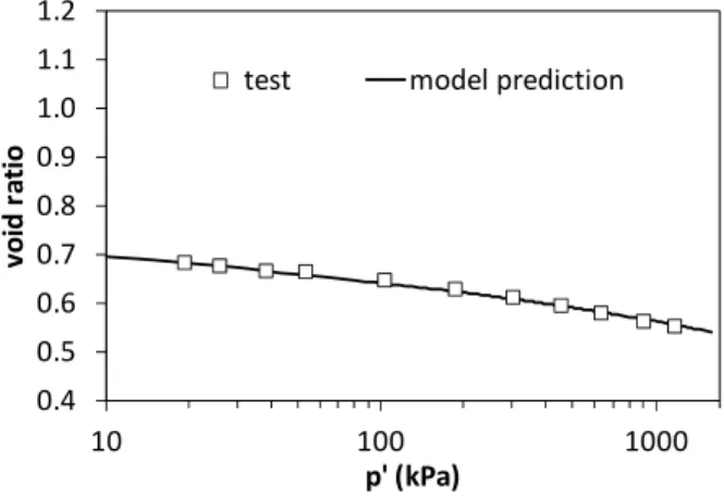
The isotropic compression test is used to determine the elastic parameters B0 and n of the one-scale
model. Fig. 9 shows the isotropic compression lines (ICL) of sand (Konishi et al. 2007). By fitting the ICL line, parameters B0 and n can be determined. For this sand, we obtain B0 = 6.53 and n =
0.8. The parameters for the proposed model fit well the experimental curve.
Another elastic parameter for the one-scale model is Poisson’s ratio, which can be estimated from the axial and volumetric strains measured in a triaxial compression test, as discussed by many researchers. For Japanese silica sand Poisson’s ratio can be taken as 0.15.
.
.
.
.
.
.
.
iti
al
v
oi
d
at
io
p' kPa
Figure 9: Simulated and measured values of Isotropic Compression Lines for silica sand tested.
3.4.3 Plastic Parameters
After the 3 elastic parametersB0,
n
and have been determined, elastic strains can be calculatedusing equation (8) and (9), and the plastic strain can then be obtained by subtracting the elastic part from the measured total strain.
Parameter D: Parameter D can be obtained from the initial slope of the p~ p v r
curve. Fig. 10 is the p ~ p
v r
curve for Japanese silica sand sample under triaxial shear (Konishi et al. 2007) with a confining pressure of 400kPa. The measured initial slope of the curve, p/ p
v r
, is -1.67, then D can be determined by Eq. (11) taking q/p=0. Using M =1.243, the value D =1.67/1.243=1.35. The average value of D = 1.2 for different confining pressures, which was later used in model prediction.
Figure. 10.Determination of parameter D
Parameter : For the proposed model, the initial slope of ~ p r
q curve is p
G . The parameters by
definition can be obtained by p/
G B
, where the value of B is calculated by Eq. (10), i.e.,
0 /
n ref
BB p p . For example, Fig. 11 is rp~q curve of the undrained triaxial compression test for
. . . . . . . . .
vo
id
a
tio
p' kPa
test odel p edictio
-0.0080 -0.0060 -0.0040 -0.0020
0.0000 0 0.01 0.02 0.03 0.04
εv
p
εp
0.86.65 400/101.35 19.58
B MPa,then the value of
can be determined by
Gp/B5.87 .The average value of
6.0 for different confining pressures was later used in model prediction.Figure. 11. Determination of parameter
Parameter m : Parameter m can be calculated from equation (14) involving four parameters: the friction angle at peak p, the critical void ratio
e
cr, the void ratioe
at peak, and the critical state friction angle cs. Among the 4 parameters,e
cr and
cs can be obtained from the known critical state parameters. The values of void ratioe
and the friction angle p can be obtained from the measured data in an undrained triaxial test. For example, from the experimental data, we obtaine
=0.66, and Mp=1.60 at peak stress state for Japanese silica sand sample (Konishi et al. 2007). Usingthe critical state parameters, we obtain
e
cr=0.687 and
cs=30.96o, then we can calculate m =3.76
using Eq. (14). The averaged value of m = 4.0 for different confining pressures was later used in model prediction.
3.4.4 Other Three Parameters for Sand-Silt Mixture
As motioned in section 3.3, these three additional parameters can be determined by fitting Eqs. (26)- (27) and (30) to triaxial tests data for mixtures with different fines content. For example, these three material constants are estimated as a=-0.3, b=0.3 and =-2.5 for Japanese silica sand-marine silt mixtures (see figure 7).
4 COMPARISON THE PREDICTED RESULTS FROM THE PROPOSED MODEL WITH SAND AND SAND-SILT MIXTURES TEST
Three sets of data of sand and sand-silt mixtures are chosen to evaluate the performance of the proposed model. One is a typical set of drained tests on Sacramento River sands (Lee and Seed 1967) , the other two tests are a set of undrained tests on Japanese silica sand-marine silt mixtures (Konishi et al., 2007) and Hokksund sand-Chengbei silt mixtures (Yang, 2004).
. . . .
Test data i itial slope Ko ishI et al.
εp
/k
4.1 Drained Test on Sacramento River Sands
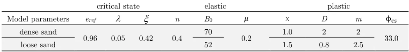
The experimental results were conducted on soil samples with two different void ratios: e = 0.87 for loosely packed sand, and e = 0.61 for densely packed sand. The model parameters are given in Ta-ble 2. The simulation results of the proposed model compared with the experimental results are shown in Fig.12.
critical state elastic plastic
Model parameters eref
n B0 χ D m ϕdense sand
0.96 0.05 0.42 0.4 70 0.2 1.0 2 2 33.0
loose sand 52 1.5 0.8 2.5
Table 2: Parameters used in the simulation for the experimental results of Sacramento River Sand.
One can see from Fig.12 that at the small strain range, the results predicted from the proposed model give good agreement with the test data. At large strain range, the predicted curves using the model give lower values of stress and volume dilation for a given strain level. Overall, the proposed model can capture the main characteristics of the stress-strain and dilatancy behavior of sand for different densities and confining pressures, for example, the dilation increases with the soil density and the contraction increases with the confining pressure.
Figure 12: Comparisons of the predictions of model and the measurement of stress-strain behavior for Sacramento Sand.
k
Pa
Axial st ai %
σ = kPa σ = kPa σ = kPa
─── odel e= .
‐ ‐
Vo
lu
et
i
st
ai
%
Axial st ai %
σ = kPa σ = kPa σ = kPa
e= . ─── odel
k
Pa
Axial st ai % σ = kPa
σ = kPa
σ = kPa
σ = . kPa
─── odel
e= .
‐ ‐ ‐ ‐ ‐ ‐ ‐
Vo
lu
et
i
st
ai
%
Axial st ai % σ = kPa
σ = kPa
σ = kPa
σ = . kPa
e= .
4.2 Undrained Tests on Japanese Silica Sand-Marine Silt Mixtures (Konishi et al., 2007)
Konish (Konishi et al., 2007) conducted a series of undrained monotonic triaxial tests on mixtures of Japanese silica sand and marine silt. Three samples with the same fines content were prepared and were compressed to large axial strains after consolidation under three different confining pres-sures (i.e. 100, 200, and 400 kPa). The stress-strain responses of the mixtures were then obtained for mixtures with different fines content.
As discussed in section 3.3, the set of parameters for any given amount of fines content can be predicted from the two sets of parameters; one for pure sand and another for pure silt. Three mate-rial constants (a, b and) to determine the parameters,
cs and ecr. For Japanese silica sand-marine silt mixtures, Three material constants are estimated as a=-0.3, b=0.3 and =-2.5. The parameters of pure sand and pure silt involved in simulation are summarized in table 3.critical state elastic plastic
Model parameters eref
n B0 χ D m φPure sand 0.68 0.016
0.82 0.8 6.53 0.15 6 1.2 4 30.96
Pure silt 1.25 0.031 3.78 8 2.0 34.99
Table 3: Parameters used in simulation for Japanese silica sand and marine silt mixtures (konish, 2007).
The simulation results of the proposed model versus experimental tests for fine contents 5%, 15%, 50% and 100% are presented in Fig. 13. For all fine contents, one can see from the stress-strain curves that the proposed models give good predictions comparing with the test data at the small strain stage. At large strain stage, the predicted curves from the one-scale model gives lower values. The predicted results of stress paths from the proposed models are in reasonable agreement to the experimental results.
4.3 Undrained Tests on Hokksund Sand-Chengbei Silt Mixtures (Yang, 2004)
A series of undrained triaxial tests on Hokksund sand mixed with different amount of Chengbei silt were conducted by Yang (2004). The consolidation confining pressures are 50, 100, and 150 kPa
respectively. All samples were compressed to large axial strains to reach steady state condition if possible. Some samples collapsed in test at lower axial strains because static liquefaction occurred during monotonic loading.
Figure 13: Stress-strain curve for Japanese silica sand-marine silt mixtures: tests and model predictions.
k
Pa
Axial st ai % % fi es co te t
= kPa
= kPa
= kPa
─── odel
k
Pa
p' kPa % fi es co te t
= kPa
= kPa
= kPa
─── odel
k
Pa
Axial st ai % % fi es co te t
= kPa
= kPa
= kPa
─── odel
k
Pa
p' kPa % fi es co te t
= kPa
= kPa = kPa
─── odel
k
Pa
Axial st ai % % fi es co te t
= kPa
= kPa
= kPa ─── odel
k
Pa
p' kPa % fi es co te t
= kPa
= kPa
= kPa
─── odel
k
Pa
Axial st ai % % fi es co te t
= kPa
= kPa = kPa
─── odel
k
Pa
p' kPa
% fi es co te t = kPa
= kPa = kPa
critical state elastic plastic Model
param-eters eref
n B0 χ D m φPure sand 0.94 0.106
0.14 0.15 13.33 0.25 4.81 0.72 4 44
Pure silt 1.25 0.227 4.22 12 1.0 27.92
Table 4: Parameters used in simulation for Hokksund sand-Chengbei silt mixtures (Yang, 2004).
One can see from Fig.14 that at the initial portion of stress-strain curve, the predicted values have a good agreement with the test data. With the development of strain, for the samples with lower fines content (i.e.0%-25%), the predicted results from the model do not match the peak stress well for confining stress of 150 kPa. However, the predicted results of stress-paths have the same trend as the stress-strain curve for the samples with lower fines content.
For the samples with fines content of 50%-95%, the predicted peak stress from the proposed one-scale model gives lower values. The predicted results of stress-paths are roughly agreed with the test results.
Experimental results show that, after peak stress, the residual shear strength reduced to almost null for fines content greater than 20%, which has significant consequences in geotechnical engineer-ing design. This is so called instability in sand and sand-silt mixtures and this post-peak behavior can be captured by the proposed model.
5 SUMMARY AND CONCLUSIONS
The present study focuses on the simulation of liquefaction behavior of granular materials such as sand and sand-silt mixtures. Based on a micromechanical analysis for inter-particle behavior, a sim-ple one-scale model for static liquefaction is proposed to simulate the stress-strain response of granular materials; the results of the analysis show the following:
The proposed model has the ability to capture the main features of sand behavior. For example, different initial void ratios lead to contracting or dilating behaviors of the sand under different drained conditions. The strain response envelopes and two-order work predicted from the model shows that the proposed one-scale model can be used to analyze the instability liquefaction of gran-ular materials.
The predicted results of triaxial test of sand and sand-silt mixtures with different fine content, which has a good agreement with the results of laboratory tests, suggest that the proposed constitu-tive model in this paper can simulate static liquefaction behavior of sand or sand-silt mixtures.
k
Pa
Axial st ai %
% fi es co te t = kPa
= kPa
= kPa
─── odel
k
Pa
p' kPa % fi es co te t
= kPa
= kPa
= kPa
─── odel
k
Pa
Axial st ai %
% fi es co te t = kPa
= kPa
= kPa
─── odel
k
Pa
p' kPa % fi es co te t
= kPa
= kPa
= kPa
─── odel
k
Pa
Axial st ai % % fi es co te t = kPa
= kPa
= kPa
─── odel
k
Pa
p' kPa % fi es co te t
= kPa
= kPa
= kPa
k
Pa
Axial st ai %
% fi es co te t = kPa
= kPa
= kPa
─── odel
k
Pa
p' kPa % fi es co te t
= kPa
= kPa
= kPa
─── odel
k
Pa
Axial st ai %
% fi es co te t = kPa
= kPa
= kPa
─── odel
k
Pa
p' kPa
% fi es co te t = kPa
= kPa
= kPa
─── odel
k
Pa
Axial st ai %
% fi es co te t = kPa
= kPa
= kPa
─── odel
k
Pa
p' kPa
% fi es co te t = kPa
= kPa
= kPa
─── odel
k
Pa
Axial st ai %
% fi es co te t = kPa
= kPa
= kPa
─── odel
k
Pa
p' kPa % fi es co te t
= kPa
= kPa
= kPa
Figure 14: Stress-strain curve for Hokksund sand-Chengbei silt mixtures: tests and model predictions.
Acknowledgements
The authors appreciate the financial support of the National Natural Science Foundation of China (No. 51178044), Beijing Higher Education Young Elite Teacher Project (YETP0340) and Beijing Excellent Talent Training Program (2013D009006000005).
References
Anderson, C.D. and Eldridge, T.L. (2012). Critical state liquefaction assessment of an upstream constructed tailings sand dam. In Tailings and Mine Waste'10 - Proceedings of the 14th International Conference on Tailings and Mine Waste, Vail, CO, United states: 101-112.
Bazier M H, Dobry R. (1995). Residual strength and large deformation potential of loose silty sands. Journal of Geotechnical Engineering Division, ASCE, 121(12):896-906.
Bedin, J. Schnaid, F.and da Fonseca, A.V. et al. (2012). Gold tailings liquefaction under critical state soil mechanics. Geotechnique, 62(3):263-267.
Bouckovalas G D, Andrianopoulos K I and Papadimitriou A G., (2003). A critical state interpretation for the cyclic liquefaction resistance of silty sands. Soil Dynamics and Earthquake Engineering, 23(2):115–125.
Boukpeti N., Drescher A. (2000). Triaxial behavior of refined Superior sand model. Computers and Geotechnics, 26:65-81.
Cambou, B., Dubujet, P., Emeriault, F., and Sidoroff, F., (1995). Homogenization for granular materials. European journal of mechanics A/Solids, 14(2): 255–276.
Casagrande A. (1975). Liquefaction and cyclic deformation of sands-a critical review. Pro of the Fifth Pan American Conf on Soil Mechanics and Foundation Engineering, Buens Aires, Argitina,
Casagrande, A. (1936). Characteristics of cohesionless soils affecting the stability of earth fills. Journalof Boston Society of Civil Engineers, 23: 257-276
Casagrande, A. (1965). Role of the 'calculated risk' in earthwork and foundation engineering. The Terzaghi Lecture, Journal of the Soil Mechanics and Foundations Division, Proceedings of the ASCE, 91, SM4, 1-40.
Castro G. Seed R B. Keller T Q. and Seed H B. (1992). Steady state strength analysis of lower san femando dam slide. Journal of Geotechnical Engineering Division, ASCE, 118(GT3):406-427.
Chang C S and Meidani M., (2013). Dominant grains network and behavior of sand–silt mixtures: stress–strain mod-eling. International Journal for Numerical and Analytical Methods in Geomechanics, 37(15):2563–2589.
Chang C S and Yin Z Y., (2011). Micromechanical modeling for behavior of silty sand with influence of fine content. International Journal of Solids and Structures, 48(19): 2655–2667.
k
Pa
Axial st ai %
% fi es co te t = kPa
= kPa
= kPa
─── odel
k
Pa
p' kPa % fi es co te t
= kPa
= kPa
= kPa
Chang, C. S. and Hicher, P. Y., (2005). An Elasto-plastic Model for Granular Materials with Microstructural Con-sideration. International Journal of Solids and Structures, 42: 4258-4277.
Chang, C. S., Sundaram, S. S., and Misra, A., (1989). Initial moduli of particulated mass with frictional contacts. International Journal for Numerical and Analytical Methods in Geomechanics, 13(6): 629-644.
Chang, C.S., (1988). Micromechanical modeling of constructive relations for granular material. In: Satake, M., Jen-kins, J.T. (Eds.), Micromechanics of Granular Materials: 271–279.
Dafalias, Y. and Herrmann, L.(1982). Bounding surface formulation of soil plasticity. In Pande, G. and Zienkiewicz, O., editors, Soil mechanics-transient and cyclic loads: 253-282, Wiley, London, 1982.
Daouadji, A, Hicher, P.-Y, Jrad, M. et.al., (2013). Experimental and numerical investigation of diffuse instability in granular materials using a microstructural model under various loading paths. Géotechnique, 63(5): 368-381.
Dash, H.K, Sitharam, T.G., (2011). Undrained Cyclic and Monotonic Strength of Sand-Silt Mixtures. Geotechnical and Geological Engineering, 29(4): 555-570.
Desai, C. and Siriwardane, H., (1984). Constitutive laws for engineering materials (with emphasis on geologic materi-als). Printice-Hall, Eaglewood Cliff, NJ.
Doanh, T., (2000). Strain Response Envelope: A complementary tool for evaluating hostun sand in triaxial compres-sion and extencompres-sion: experimental observations. In Constitutive Modelling of Granular Materials. Springer Verlag Berlin: 375-396.
Emeriault, F. and Cambou, B., (1996). Micromechanical modelling of anisotropic non-linear elasticity of granular medium. International Journal of Solids and Structures, 33 (18): 2591–2607.
Fourie A B, Papageorgiou G., (2001). Defining an appropriate steady state line for Merriespruit gold tailings. Cana-dian Geotechnical Journal, 38:695–706.
Gudehus, G., (1979). A comparison of some constitutive laws for soils under radially symmetric loading and unload-ing, in: W. Wittke (Ed.) Proc. 3rd International Conference on Numerical Methods in Geomechanics, Balkema, 1309-1323.
Hazen, A. Hydraulic fill dams. Transactions, American Society of Civil Engineers, (1920), 83: 1713-1745. Ishiraha, K. (1993). Liquefaction and flow failure during earthquakes . Géotechnique, 43(3): 351-451.
Ishiraha,K., Tatsuka,F., and Yasuda,S. (1975). Undrained deformation and liquefaction of sand under cyclic stress. Soils Found, 15(1):29-44.
James, Michael, Aubertin, Michel and Wijewickreme, Dharma. (2011). A laboratory investigation of the dynamic properties of tailings. Canadian Geotechnical Journal, 48(11): 1587-1600.
Jenkins, J. T. and Strack, O. D. L., (1993). Mean-field inelastic behavior of random arrays of identical spheres. Me-chanics of Material, 16: 25-33.
Jenkins, J. T., (1988). Volume change in small strain axisymmetric deformations of a granular material. In: Satake, M., Jenkins, J.T. (Eds.), Micromechanics of Granular Materials: 143-152.
Klisinski, M., (1988). Plasticity theory based on fuzzy sets. Journal of Engineering Mechanics, 114(4):563-582. Kolymbas, D., (2000). Response-Envelopes: a useful tool as "Hypoplasticity then and now". In D. Kolymbas (Ed.), Constitutive Modelling of Granular Materials. Berlin: Springer-Verlag, 57-105.
Konishi, Y., Hyodo M., and Ito, S., (2007). Compression and undrained shear characteristics of sand-fines mixtures with various plasticity. JSCE J. Geotech. Eng. & Geoenviron. Eng, 63(4): 1142-1152 (in Japanese).
Kruyt, N. P. and Rothenburg, L., (2002). Micromechanical bounds for the effective elastic moduli of granular mate-rials. International Journal of Solids and Structures, 39 (2):311-324.
Kuerbis, R.H, Nagussey, D., Vaid, Y.P., (1998). Effect of gradation and fines content on the undrained response of sand. In: Proceedings of Hydraulic Fill Structures.Geotech. Spec. Publ. 21, ASCE, New York, pp. 330-345.
Lade P V., (1992). Static instability and liquefaction of loose fine sandy slopes. Journal of Geotechnical Engineering, 118(1):51-71.
Lade P.V., Yamamuro, J.A., (1997). Effect of non-plastic fines on static liquefaction of sands. Canadian Geotechnical Journal, 34 (6): 917-928.
Lade, P V. and Yamamuro, Jerry A. (2011) Evaluation of static liquefaction potential of silty sand slopes. Canadian Geotechnical Journal. 48(2): 247-264.
Lee, K.L and Seed, H.B., (1967). Draind strength characteristics of sands. Journal of the Soil Mechanics and Foun-dations Division, SM6:117-141.
Lewin, P. and Burland, J., (1970). Stress-probe experiments on saturated normally consolidated clay. Géotechnique, 20 (1):38-56.
Liao, C. L., Chan, T. C., Suiker, A. S. J., et al., (2000). Pressure-dependent elastic moduli of granular assemblies. International Journal for Numerical and Analytical Methods in Geomechanics, 24: 265-279.
Maleej, Y., Dormieux, L., and Sanahuja, J., (2009). Micromechanical approach to the failure criterion of granular media. European J. Mechanics A/Solids, 28:647-653.
Matsuoka, H. and Takeda, K., (1980). A stress–strain relationship for granular materials derived from microscopic shear mechanisms. Soils & Foundation, 120 (3): 45-58.
Misra A and Singh V., (2014). Nonlinear granular micromechanics model for multi-axial rate-dependent behavior, International Journal of Solids and Structures, 51:2272-2282.
Misra, A. and Yang, Y., (2010). Micromechanical model for cohesive materials based upon pseudo-granular structure. International Journal of Solids and Structures, 247:2970-2981.
Mitchell J K., (1993). Fundamentals of soil behavior, 2nd edn. Wiley Interscience Publication.
Monkul, M M, Yamamuro, J A., (2011). Influence of silt size and content on liquefaction behavior of sands. Canadi-an Geotechnical Journal, 48(6): 931-942.
Mro´z , Z.,NBoukpeti, N and Drescher, A. (2003). Constitutive Model for Static Liquefaction. International Journal of Geomechanics, International Journal of Geomechanics, 3(2):133-144.
Murthy, T.G., Loukidis, D., Carraro, J.A.H., et al., (2007). Undrained monotonic response of clean and silty sands. Géotechnique, 57 (3): 273–288.
Ni, Q., Tan, T.S., Dasari, G.R.,et al., (2004). Contribution of fines to the compressive strength of mixed soils. Géotechnique, 54 (9):561–569.
Nicot F, Darve F., (2006). Micro-mechanical investigation of material instability in granular assemblies. International Journal of Solids and Structures, 43(11-12):3569–3595.
Nicot, F. and Darve, F., (2007). Basic features of plastic strains: From micro-mechanics to incrementally nonlinear models. International Journal of Plasticity, 23:1555-1588.
Pitman, T.D., Robertson, P.K., Sego, D.C., (1994). Influence of fines on the collapse of loose sands. Canadian Ge-otechnical Journal, 31 (5):728–739.
Polulos S J. (1981). The steady state of deformation. Journal Geotechnical engineering, ASCE, 107(5):553-562. Polulos S J. (1985). Liquefaction evaluation procedure. J Geotecnical engineering Division, ASCE, 111(GT6):772-792. Prevost Prevost, J., (1985). A simple plasticity theory for cohesioless soils. Soil Dynamics and Earthquake Engineer-ing, 4(1): 9-17.