A Regional Climate Simulation Study Using WRF-ARW Model over Europe and Evaluation for Extreme Temperature Weather Events

Research Article

A Regional Climate Simulation Study Using WRF-ARW

Model over Europe and Evaluation for Extreme Temperature

Weather Events

Hari Prasad Dasari,

Rui Salgado,

Joao Perdigao,

and Venkata Srinivas Challa

2_{Departamento de F´ısica, Centro de Geof´ısica, Escola de Ciˆencias e Tecnologia, Universidade de ´Evora, 7000 Evora, Portugal} 3_{Radiological Safety and Environment Group, Indira Gandhi Center for Atomic Research, Kalpakkam 603102, India} Correspondence should be addressed to Hari Prasad Dasari; [email protected]

Received 7 April 2014; Revised 3 July 2014; Accepted 4 July 2014; Published 2 September 2014 Academic Editor: Helena A. Flocas

Copyright © 2014 Hari Prasad Dasari et al. This is an open access article distributed under the Creative Commons Attribution License, which permits unrestricted use, distribution, and reproduction in any medium, provided the original work is properly cited.

In this study regional climate simulations of Europe over the 60-year period (1950–2010) made using a 25 km resolution WRF model with NCEP 2.5 degree analysis for initial/boundary conditions are presented for air temperature and extreme events of heat and cold waves. The E-OBS 25 km analysis data sets are used for model validation. Results suggest that WRF could simulate the temperature trends (mean, maximum, minimum, seasonal maximum, and minimum) over most parts of Europe except over Iberian Peninsula, Mediterranean, and coastal regions. Model could simulate the slight fall of temperatures from 1950 to 1970 as well as steady rise in temperatures from 1970 to 2010 over Europe. Simulations show occurrence of about 80% of the total heat waves in the period 1970– 2010 with maximum number of heat/cold wave episodes over Eastern and Central Europe in good agreement with observations. Relatively poor correlations and high bias are found for heat/cold wave episodes over the complex topographic areas of Iberia and Mediterranean regions where land surface processes play important role in local climate. The poor simulation of temperatures over the above regions could be due to deficiencies in representation of topography and surface physics which need further sensitivity studies.

1. Introduction

Climate change is a widely discussed environmental issue in recent times. Increase in the greenhouse gases due to consumption of fossil fuels, increase in deforestation, and anthropogenic activities have been attributed as the causes for the present changes in the temperature and rainfall

patterns [1–4]. Variations in temperature and precipitation

on global, regional, and local scales are the issues of interest for their impact on the ecosystem. The projections of mean atmospheric temperature and precipitation during the 21st century indicate ecological, economic, and social disruptions are likely to occur in the future. Some of the projected

changes [5] in European climate include (i) increase of water

vapour transport from low to high latitudes, (ii) changes in atmospheric circulation on longer time scales, (iii) reduction of snow cover during winter in the northeastern part of the

continent, (iv) drying of the soil in summer in the Mediter-ranean and Central European regions, and (v) increase in annual mean temperatures with higher warming in winters in northern Europe and in summers in the Mediterranean area. Studies indicate that the increase of annual mean temperature over Europe will exceed the global warming rate in the 21st century. Studies indicate that temperatures in winter

would increase in northern Europe [6], and temperatures

during summer would increase in the Mediterranean area.

Hanssen-Bauer et al. [7] have reported that during winter

minimum temperatures would increase more than the mean temperature in northern Europe. A recent study by Tebaldi

et al. [8] reported that maximum temperatures in summer

are likely to increase more than the mean summer temper-ature in southern and Central Europe. Climate variability on interannual time scale is crucial to understand climate

impacts on agricultural production systems [9]. The dra-matic economic and societal repercussions of the extreme European summer of 2003 and 2010 clearly demonstrate the

climate change impacts [10–12]. Atmosphere-ocean coupled

general circulation models (AOGCM) facilitate to study

large-scale climate extreme events [5]. However, small-scale

extreme weather events cannot be resolved by AOGCMs. Regional climate models (RCM) can be used to dynam-ically downscale and obtain small-scale regional climate

information from global climate models [13–16]. Several

studies demonstrated the advantages of regional models, with higher spatial and temporal resolution, for regional climate prediction by suitably integrating them with the

boundary conditions provided by the AOGCMs [17–20]. The

RCMs provide localized, high resolution information and can simulate the effects of complex topography with large land-water contrasts to derive regional climate consistent with the large-scale climate simulated by the AOGCM used as forcing

[21].

A number of models such as RegCM, CSU/RAMS, and UKMO have been developed for regional climate studies

[22–27]. RCMs due to both higher resolution and improved

physics are able to better resolve mesoscale effects associated with topography (coastlines, mountains, water bodies, veg-etation etc.,), the local climate, and the related influence on

the temperature and precipitation systems ([28–38] among

others). The ENSEMBLES project in Europe deals with the scientific aspects of regional climate change and with

the objectives of understanding model uncertainties [39].

Some of the studies in the project are focused on the skill of the model performance with respect to precipitation and temperature over different parts of Europe and also

Europe as a whole [36, 40–47]. A few studies attempted

the long-term climate investigation on a regional scale at a high resolution using WRF over certain specific regions or

complex topographic areas in Europe [48, 49] for limited

period of about 2 to 3 decades. However, an analysis of temperature variations over various parts requires long-term simulations over entire Europe using regional models with a computationally affordable resolution.

The objective of this work is to study the fidelity of Advanced Research Weather Research and Forecast (WRF-ARW) regional model to simulate the temperature patterns in Europe over the 60-year period (1950–2010) with reference to the warm and cold seasons, their long-term variability, and subregional variations and to improve the knowledge of the temperature variations, especially of the extreme heat/cold wave events on a regional scale over Europe. The WRF-ARW regional model is chosen as it has the sophisticated physics for land-surface, planetary boundary layer, radiation, and other atmospheric processes that are important to simulate the regional small-scale processes.

2. Model and Data

ARW is a limited area, primitive equation, nonhydrostatic, and terrain following sigma coordinate model. The model is configured with two-way interactive nested domains with

horizontal grid spacing of 75 km in the outer domain

and 25 km in the inner domain (Figure 1). The details

of model domains and physics are presented in Table 1.

The outer domain covers the region encompassing the entire Europe and parts of Atlantic Ocean, Southern Arctic, and so forth. The three-dimensional initial atmospheric fields and the time varying boundary conditions are derived from the National Centers for Environmental Prediction

(NCEP) global reanalysis fields [50] available at 2.5 degree

latitude/longitude resolution and at 6-hour interval. The model is integrated continuously for 13 months, starting from 00UTC of 1 May for each year from 1950 for the entire 6 decades of 1950–2010; although model can be initialized in any season during a year, we have chosen 00UTC 1 May as starting time as it corresponds to a summer weak synoptic condition over Europe. The model outputs are generated at every 3-hour interval and model results are analyzed from the 25 km resolution domain. The first one month simulation of each year run is considered as model spinup time and hence neglected from analysis. The model physics is chosen

as the WSM3 explicit microphysics, Dudhia scheme [51]

for shortwave radiation processes, RRTM scheme for long

wave radiation processes [52], the nonlocal YSU scheme for

PBL turbulence [53,54], multilayer soil scheme for surface

processes, and the Betts-Miller-Janjic [55,56] for convection.

The soil scheme solves the thermal diffusivity equation using 5 soil layers and the energy budget includes radiation, sensible, and latent heat fluxes. It treats the snow-cover, soil moisture as fixed quantities with a land use and season-dependent constant value. The terrain, land use, and soil data are interpolated to the model grids from USGS global elevation, 24 category USGS vegetation data and 17 category FAO soil data with suitable spatial resolution (arc 5 minutes) to define the lower boundary conditions. The maximum and minimum temperatures are computed from the 3-hour interval outputs. The model results for the whole 60-year

period (1950 to 2010) are compared with E-OBS V7.0 [57]

observations available at 0.25 degree. The E-OBS is the only source of data available in the public domain for comparative analysis. As E-OBS data has the same resolution (25 km) as that of ARW 2nd domain no interpolation is applied while comparing the results. Also no corrections for bias in E-OBS data have been applied. Spatial statistics between observa-tions and model produced mean, minimum, and maximum temperatures are generated for entire period as a whole and on different seasons. The number of heat waves and cold waves is computed from E-OBS data and simulations and discussed.

3. Statistical Methods

In the present study the framework of model evaluation

by Murphy and Winkler [58] is followed. To assess the

long-term performance several statistical indices are esti-mated. They include Pearson correlation coefficient (COR), normalized BIAS (NBIAS), normalized root mean square error (NRMSE), normalized mean absolute error (NMAE),

(a) 0 50 250 500 750 0 1500 1750 13 42 5 6 7 8 9 10 11 12 13 14 15 10 ∘ W ∘₅W 0 ∘₅E ∘ ₁₀E ∘₁₅E ∘₂₀E 54N 52∘N 50∘N 48∘_N 46∘_N 44∘N 42∘N 40∘_N 38∘_N 36∘N 34∘N 32∘_N (b)

Figure 1: (a) Model domains used for this study (b) topography along with chosen region.

Table 1: Model details and configuration.

Model name NCEP/NCAR ARW

Model type Primitive equation, nonhydrostatic Vertical resolution 30 sigma levels; model top—10 hPa Horizontal resolution 75 km 25 km Domain of integration 38.5W-30.83E 13.585W-24.8351E

21.82N-59.75N 31.7935N-55.7455N Radiation scheme CAM scheme for short wave radiation.

CAM scheme for long wave radiation Land-surface scheme Thermal diffusion scheme Sea surface temperature Real sea surface temperatures Convection scheme Grell-Devenyi ensemble scheme

PBL scheme YSU scheme

Explicit moisture scheme WSM 3-class simple ice scheme

and normalized standard deviation (NSTDEV) as given below: COR= ∑ 𝑛 𝑖=1(𝑓𝑖− 𝑓) (𝑜𝑖− 𝑜) √∑𝑛 𝑖=1(𝑓𝑖− 𝑓)2√∑𝑛𝑖=1(𝑜𝑖− 𝑜)2 , ₍₁₎ BIAS= 1 𝑛 𝑛 ∑ 𝑖=1 (𝑓_𝑖− 𝑜_𝑖) = 𝑓 − 𝑜, (2) STDEV = √𝑆2_𝑓+ 𝑆2_𝑜− 2𝑆_𝑓𝑆_𝑜𝑟_𝑓𝑜, (3) RMSE= √(∑ 𝑛 𝑖=1(𝑓𝑖− 𝑜𝑖)2) 𝑛 , (4) MAE= 1 𝑛 𝑛 ∑ 𝑖=1󵄨󵄨󵄨󵄨𝑓𝑖 − 𝑜_𝑖󵄨󵄨󵄨󵄨, (5)

RANGE= (𝑜_{max,𝑖=1,𝑛}− 𝑜_{min,𝑖=1,𝑛}) . (6)

From (2) to (5), the normalized values for each statistical

index can be obtained by the following formulas:

NBIAS= ( BIAS RANGE) × 100, NSTDEV= (STDEV RANGE) × 100, NRMSE= ( RMSE RANGE) × 100, NMAE= ( MAE RANGE) × 100. (7)

Also another coefficient called Nash-Sutcliffe efficiency (NSE) coefficient commonly employed to assess the pre-dictive power of hydrological model is also evaluated. It is defined as

NSE= 1 − ((1/𝑛) ∑

𝑛

𝑖=1(𝑓𝑖− 𝑜𝑖)2)

((1/𝑛) ∑𝑛_𝑖=1(𝑓_𝑖− 𝑓)2), (8)

where𝑂_𝑖 is an observed variable,𝑓_𝑖 is a modeled variable,

overbar represents average over all the data, and “𝑛” is the total number of locations that predicted data are compared against observations. Bias is a measure of mean error for a continuous variable, SD is the standard deviation of the

error (𝑓-𝑜), where 𝑆_𝑓 is the standard deviation in

fore-casts,𝑆_𝑜 is the standard deviation in observations, and𝑟_𝑓𝑜

is the correlation between the forecasts and observations. The Nash-Sutcliffe efficiency (NSE) coefficient ranges from negative infinity to one. An efficiency of 1 corresponds to a perfect match between observed and modeled values. The

NSE ranges 0–0.3, 0.3–0.6, 0.6–0.8, and >0.8 indicate the

model performance is poor, reasonable, good, and excellent,

respectively [59,60]. Specifically, MAE is less influenced by

large errors and also does not depend on the mean error. The normalized values of BIAS, STDEV, and MAE are often expressed in percentages. The NBIAS is a measure of the over- or underprediction of a variable. Positive values indicate overprediction and negative values indicate underprediction. Similarly NSTDEV and NMAE are also expressed in percent-ages but with smaller values representing better agreement

between observed and modelled values. In this study we used the COR, NBIAS, NMAE, and NSTDEV to validate the model performance against observations.

4. Results and Discussion

The results are presented in three sections. The first section focuses on 60-year mean values of minimum, maximum, and mean temperatures and corresponding spatial statistics between E-OBS (referred hereafter as observations) and corresponding model values. In the second section the sea-sonal means for winter (December, January, and February), spring (March, April, and May), summer (June, July, and August), and autumn (September, October, and November) are produced for all 6 decades and model performance evaluated by comparisons with corresponding observations. Finally, a comparative analysis is made over different zones in

Europe for heat waves and cold waves (Figure 1). A total of 15

zones are considered for the extreme value analysis wherein the zones are selected based on characteristics of topography. These different zones are distributed over Iberian Peninsula, Mediterranean region, Central Europe, and Eastern Europe. Zones 6–8 and 13-14 are located in the northern and western

Europe with moderate altitude of ≤250 m above mean sea

level (AMSL), zones 2–5 are located in Iberian Peninsula with mean altitude of 250 to 1000 m AMSL, zones 10 and 11 are located in the high altitude (≥1500 m AMSL) Alps mountain region, and zone 12 with moderate altitude is located in the Italian peninsula. The heat wave conditions are analysed from daily maximum temperatures from summer months and cold waves from daily minimum temperatures of winter seasons as per their definition prescribed by World Meteorological

Organization [61].

4.1. Analysis of Daily Temperatures. The daily mean,

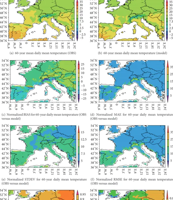
max-imum, and minimum temperatures from simulation and observations are presented in this section. The spatial dis-tribution of 60-year mean daily mean temperatures and

corresponding model values is presented in Figures2(a)and

2(b). It is seen that the spatial distribution of model mean

temperatures is in good agreement with observations. Lesser temperatures are noted over Iberian Peninsula relative to observations. Normalized values of BIAS, MAE, STDEV, and RMSE between model and observed mean daily temperatures

for entire 60-year period are presented in Figures2(c)and

2(f). The spatial NBIAS distribution (Figure 2(c)) indicates

the model underestimates air temperature by around −5

to −10% over the Iberian Peninsula and overestimates air

temperatures by +15% over Alps Mountain. In other parts

of Europe the bias is about−5 to 5%. Similarly the NMAE

over Iberian Peninsula region is about 5–10% and about 10–

25% over Alps region (Figure 2(d)). The NSTDEV between

observed and model simulated mean temperatures is about 5–10% in most of Europe except the coast line in Eastern

Europe where the NSTDEV is about ∼20% (Figure 2(e)).

The NRMSE in mean temperature is about 10–15% over the Iberian Peninsula and 15–25% over Alps, a few areas in Italy and Iberia, while the rest of Europe has NRMSE

of 5–10% (Figure 2(f)). The spatial temperature correlations

(Figure 2(g)) obtained at 99% significance indicate high correlations (>0.9) in Eastern Europe, moderate correlations (0.85–0.9) in western and central parts, and relatively less correlations (0.7–0.8) in coastal parts. The low correlations are associated with high NSTDEV as expected. Overall reasonably good correlations (>0.7) are obtained for surface air temperature over most parts of Europe. All the above statistical indices clearly show that the model simulated daily mean temperatures fairly well in the central and eastern parts of the domain and moderately well over the western parts especially over the Iberian Peninsula. This is reflected in the Nash coefficient (0.1–0.3 poor; 0.3–0.6 good; more than 0.6 very good) which has poor values (0.01 to 0.3) over coastal parts and Iberian region and moderate values (0.3–0.6) over Central and southeastern Europe and higher values (>0.6) over northeastern Europe. The obtained Nash coefficient (Figure 2(h)) values indicate the model performance is fairly

good over most parts of Europe with values of ≥0.3 and

relatively poor over Alps region and few west coastal parts The above results indicate the model produces a warm bias in the Eastern Europe, Alps, and few central parts, and cold bias over most of Iberian Peninsula, Italy, and many western parts.

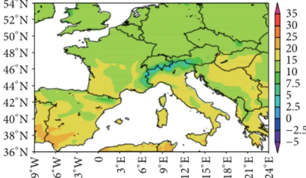
To examine the simulation of time cycle of temperatures we analysed the maximum and minimum daily temperatures

(in Figures3and4). The spatial patterns of simulated mean

daily maximum and mean daily minimum temperatures are noted to be in good agreement with those derived from observations. The model slightly underestimates maximum temperature over Iberian region and simulates well over other

parts of Europe (Figures3(a)and 3(b)). The NBIAS values

are in the range of −10 to 10% over most of Europe. The

NBIAS indicates a cold bias (−5 to −10%) over Iberia, slight cold bias (−5%) over western and northern parts, and slight warm bias (5%) over western Europe, western parts of Italy, and few zones such as Alps. Similarly from other statistical

parameters NSTDEV and NRMSE (Figures3(e)and3(f)) it is

seen that the normalized errors are less than 10% in most parts of Europe except Iberian Peninsula and Alps region which have normalized RMSE in the range 10–15% and 15–25%, respectively. Spatial correlations for maximum temperature are fairly good (>0.85) over most parts of Europe except the northwestern areas, western coastal areas, and Alps which have correlations in the range 0.7–0.85. Correspondingly the Nash coefficient is also poor (<0.01) over limited parts of Iberia and Alps indicating poor simulation of maximum temperatures over those areas. However, the Nash coefficient

values (Figure 3(h)) for maximum temperatures are higher

relative to mean temperatures. All the above indices show that the simulations for maximum temperature are good over most parts of Iberia and western and Central Europe and rel-atively better in Eastern Europe. The Correlation coefficient (Figure 3(g)) values are high (>0.8) over most of the domain

with 95% significance except the west coast of Europe which has slightly lesser correlations (∼0.7). Similar spatial trends are noted in 60-year mean daily minimum temperatures

(Figures4(a)and4(b)) as with maximum temperatures. In

−5 −2.5 0 2.5 5 7.5 10 15 20 30 35 25 3 ∘ W 6 ∘ W 9 ∘ W 0 ∘ 3E ∘ 6E ∘ 9E ∘ ₁₂E ∘ ₁₅E ∘₁₈E ∘₂₁E ∘₂₄E 54∘_N 52∘N 50∘_N 48∘_N 46∘N 44∘N 42∘_N 40∘_N 38∘N 36∘N

(a) 60-year mean daily mean temperature (OBS)

−5 −2.5 0 2.5 5 7.5 10 15 20 30 35 25 3 ∘ W 6 ∘ W 9 ∘ W 0 ∘ 3E ∘ 6E ∘ 9E ∘ ₁₂E ∘₁₅E ∘₁₈E ∘₂₁E ∘₂₄E 54∘_N 52∘N 50∘N 48∘_N 46∘N 44∘N 42∘_N 40∘N 38∘N 36∘_N

(b) 60-year mean daily mean temperature (model)

−25 −15 −10 −5 0 5 10 15 25 3 ∘W 6 ∘W 9 ∘W 0 ∘₃E ∘₆E ∘₉E ∘₁₂E ∘₁₅E ∘₁₈E ∘₂₁E ∘₂₄E 54∘_N 52∘_N 50∘N 48∘N 46∘_N 44∘_N 42∘N 40∘N 38∘_N 36∘_N

(c) Normalized BIAS for 60-year daily mean temperature (OBS versus model) 5 10 15 35 25 3 ∘W 6 ∘W 9 ∘W 0 ∘₃E ∘₆E ∘₉E ∘₁₂E ∘₁₅E ∘₁₈E ∘₂₁E ∘₂₄E 54∘N 52∘N 50∘_N 48∘_N 46∘N 44∘N 42∘_N 40∘N 38∘N 36∘_N

(d) Normalized MAE for 60-year daily mean temperature (OBS versus model)

5 7.5 10 12.5 15 3 ∘ W 6 ∘ W 9 ∘ W 0 ∘ 3E ∘ 6E ∘ 9E ∘ ₁₂E ∘₁₅E ∘₁₈E ∘₂₁E ∘₂₄E 54∘_N 52∘N 50∘_N 48∘_N 46∘N 44∘N 42∘_N 40∘N 38∘N 36∘_N

(e) Normalized STDEV for 60-year daily mean temperature (OBS versus model)

5 15 10 35 25 3 ∘ W 6 ∘W 9 ∘W 0 ∘ 3E ∘ 6E ∘ 9E ∘₁₂E ∘₁₅E ∘₁₈E ∘₂₁E ∘₂₄E 54∘_N 52∘N 50∘N 48∘_N 46∘N 44∘N 42∘_N 40∘_N 38∘N 36∘N

(f) Normalized RMSE for 60-year daily mean temperature (OBS versus model)

0.2 0.4 0.6 0.7 0.8 0.85 0.9 0.95 3 ∘W 6 ∘W 9 ∘W 0 ∘3E ∘6E ∘9E ∘₁₂E ∘₁₅E ∘₁₈E ∘₂₁E ∘₂₄E 54∘_N 52∘N 50∘N 48∘_N 46∘N 44∘N 42∘N 40∘_N 38∘N 36∘N

(g) Correlation coefficient for 60-year daily mean temperature (OBS versus model)

0.01 0.3 0.6 0.8 3 ∘W 6 ∘W 9 ∘W 0 ∘3E ∘6E ∘ 9E ∘ ₁₂E ∘ ₁₅E ∘ ₁₈E ∘ ₂₁E ∘ ₂₄E 54∘_N 52∘N 50∘_N 48∘_N 46∘N 44∘N 42∘_N 40∘N 38∘N 36∘_N

(h) Nash-Sutcliffe coefficient for 60-year daily mean tempera-ture (OBS versus model)

Figure 2: 60-year daily mean temperatures at 2 m height. (a) Mean from OBS and (b) mean from model and (c) normalized BIAS (%), (d) normalized MAE (%), (e) normalized STDEV (%), (f) normalized RMSE (%), (g) correlation coefficient, and (h) Nash-Sutcliffe coefficient (%) for 60-year daily mean 2 m height temperatures between OBS and model.

−5 −2.5 0 2.5 5 7.5 10 15 20 30 35 25 54∘_N 52∘_N 50∘_N 48∘N 46∘N 44∘_N 42∘_N 40∘N 38∘N 36∘_N 3 ∘ W 6 ∘ W 9 ∘ W 0 ∘ ₃E ∘ ₆E ∘₉E 12 ∘E 15 ∘E 18 ∘E 21 ∘E 24 ∘E

(a) Mean for 60-year daily maximum temperature (OBS)

54∘_N 52∘_N 50∘_N 48∘N 46∘N 44∘_N 42∘N 40∘N 38∘_N 36∘_N 3 ∘W 6 ∘W 9 ∘W 0 ∘₃E ∘₆E ∘₉E ∘₁₂E ∘ ₁₅E ∘ ₁₈E ∘ ₂₁E ∘ ₂₄E −5 −2.5 0 2.5 5 7.5 10 15 20 30 35 25

(b) Mean for 60-year daily maximum temperature (model)

−25 −15 −10 −5 0 5 10 15 25 54∘_N 52∘_N 50∘_N 48∘N 46∘N 44∘_N 42∘_N 40∘N 38∘N 36∘_N 3 ∘ W 6 ∘ W 9 ∘ W 0 ∘3E ∘6E ∘9E ∘₁₂E ∘₁₅E ∘₁₈E ∘₂₁E ∘₂₄E

(c) Normalized BIAS for 60-year daily maximum temperature (OBS versus model)

5 10 15 35 25 54∘N 52∘N 50∘N 48∘N 46∘_N 44∘N 42∘N 40∘N 38∘_N 36∘N 3 ∘W 6 ∘W 9 ∘W 0 ∘ 3E ∘ 6E ∘ 9E ∘ ₁₂E ∘ ₁₅E ∘ ₁₈E ∘ ₂₁E ∘ ₂₄E

(d) Normalized MAE for 60-year daily maximum tempera-ture (OBS versus model)

5 7.5 10 12.5 15 3 ∘W 6 ∘W 9 ∘W 0 ∘3E ∘6E ∘9E ∘₁₂E ∘₁₅E ∘₁₈E ∘₂₁E ∘₂₄E 54∘_N 52∘N 50∘N 48∘_N 46∘_N 44∘N 42∘N 40∘_N 38∘_N 36∘N

(e) Normalized STDEV for 60-year daily maximum tempera-ture (OBS versus model)

5 15 10 35 25 54∘N 52∘_N 50∘_N 48∘N 46∘N 44∘_N 42∘_N 40∘N 38∘N 36∘_N 3 ∘ W 6 ∘ W 9 ∘ W 0 ∘ 3E ∘6E ∘9E ∘₁₂E ∘₁₅E ∘₁₈E ∘₂₁E ∘₂₄E

(f) Normalized RMSE for 60-year daily maximum tempera-ture (OBS versus model)

0.2 0.4 0.6 0.7 0.8 0.85 0.9 0.95 54∘_N 52∘N 50∘_N 48∘_N 46∘N 44∘N 42∘_N 40∘_N 38∘N 36∘N 3 ∘W 6 ∘W 9 ∘W 0 ∘3E ∘6E ∘9E ∘ ₁₂E ∘ ₁₅E ∘ ₁₈E ∘ ₂₁E ∘ ₂₄E

(g) Correlation coefficient for 60-year daily maximum temper-ature (OBS versus model)

0.01 0.3 0.6 0.8 54∘N 52∘_N 50∘N 48∘N 46∘_N 44∘_N 42∘N 40∘N 38∘_N 36∘_N 3 ∘ W 6 ∘ W 9 ∘ W 0 ∘ 3E ∘ 6E ∘ 9E ∘ ₁₂E ∘ ₁₅E ∘ ₁₈E ∘ ₂₁E ∘ ₂₄E

(h) Nash-Sutcliffe coefficient for 60-year daily maximum tem-perature (OBS versus model)

Figure 3: 60-year daily maximum temperatures at 2 m height. (a) Mean from OBS and (b) mean from model and (c) normalized BIAS (%), (d) normalized MAE (%), (e) normalized STDEV (%), (f) normalized RMSE (%), (g) correlation coefficient, and (h) Nash-Sutcliffe coefficient (%) for 60-year daily mean 2 m height temperatures between OBS and model.

−5 −2.5 0 2.5 5 7.5 10 15 20 −10 12.5 17.5 54∘_N 52∘N 48∘_N 46∘N 44∘N 42∘_N 40∘_N 50∘N 38∘N 36∘N 9 ∘W ∘₆W ∘₃W 0 ∘3E ∘ 6E ∘ E9 ∘ ₁₂E ∘ ₁₅E ∘ ₁₈E ∘ ₂₁E ∘₂₄E

(a) Mean for 60-year daily minimum temperature (OBS)

−5 −2.5 0 2.5 5 7.5 10 15 20 −10 12.5 17.5 54∘N 52∘_N 48∘N 46∘_N 44∘_N 42∘N 40∘N 50∘N 38∘_N 36∘N 9 ∘W ∘₆W ∘₃W 0 ∘ 3E ∘ 6E ∘ E9 ∘ ₁₂E ∘ ₁₅E ∘ ₁₈E ∘ ₂₁E ∘ ₂₄E

(b) Mean for 60-year daily minimum temperature (model)

−25 −15 −10 −5 0 5 10 15 25 54∘_N 52∘_N 48∘N 46∘_N 44∘N 42∘N 40∘_N 50∘N 38∘_N 36∘N 9 ∘ W ∘ ₆W ∘ ₃W 0 ∘ 3E ∘ 6E ∘ E9 ∘ ₁₂E ∘ ₁₅E ∘₁₈E ∘₂₁E ∘₂₄E

(c) Normalized BIAS for 60-year daily minimum temperature (OBS versus model)

5 10 15 35 25 54∘N 52∘N 48∘_N 46∘N 44∘N 42∘_N 40∘_N 50∘N 38∘N 36∘_N 9 ∘ W ∘ ₆W ∘ ₃W 0 ∘ 3E ∘ 6E ∘ E9 ∘₁₂E ∘₁₅E ∘₁₈E ∘₂₁E ∘₂₄E

(d) Normalized MAE for 60-year daily minimum tempera-ture (OBS versus model)

5 7.5 10 12.5 15 54∘N 52∘N 48∘_N 46∘N 44∘N 42∘_N 40∘_N 50∘N 38∘N 36∘N 9 ∘W ∘₆W ∘₃W 0 ∘3E ∘6E ∘E9 ∘₁₂E ∘₁₅E ∘₁₈E ∘₂₁E ∘ ₂₄E

(e) Normalized STDEV for 60-year daily minimum tempera-ture (OBS versus model)

54∘N 52∘_N 48∘N 46∘_N 44∘_N 42∘N 40∘N 50∘N 38∘_N 36∘_N 9 ∘ W ∘ ₆W ∘ ₃W 0 ∘ 3E ∘ 6E ∘ E9 ∘₁₂E ∘₁₅E ∘₁₈E ∘₂₁E ∘₂₄E 5 10 15 35 25

(f) Normalized RMSE for 60-year daily minimum tempera-ture (OBS versus model)

0.2 0.4 0.6 0.7 0.8 0.85 0.9 0.95 54∘_N 52∘N 48∘N 46∘_N 44∘N 42∘N 40∘_N 50∘N 38∘_N 36∘N 9 ∘ W ∘ ₆W ∘ ₃W 0 ∘ 3E ∘ 6E ∘ E9 ∘ ₁₂E ∘₁₅E ∘₁₈E ∘₂₁E ∘₂₄E

(g) Correlation coefficient for 60-year daily minimum temper-ature (OBS versus model)

0.01 0.3 0.6 0.8 54∘N 52∘_N 48∘N 46∘N 44∘_N 42∘_N 40∘N 50∘_N 38∘N 36∘_N 9 ∘ W ∘ ₆W ∘ ₃W 0 ∘ 3E ∘ 6E ∘ E9 ∘ ₁₂E ∘₁₅E ∘₁₈E ∘₂₁E ∘₂₄E

(h) Nash-Sutcliffe coefficient for 60-year daily minimum tem-perature (OBS versus model)

Figure 4: 60-year daily minimum temperatures at 2 m height. (a) Mean from OBS and (b) mean from model and (c) normalized BIAS (%), (d) normalized MAE (%), (e) normalized STDEV (%), (f) normalized RMSE (%), (g) correlation coefficient, and (h) Nash-Sutcliffe coefficient (%) for 60-year daily mean 2 m height temperatures between OBS and model.

underestimation of minimum temperatures is about 0–5% indicating slight clod bias over these areas. To assess the errors in the simulation of minimum temperatures we analyzed the NBIAS, NMAE, NSTDEV, and NRMSE. The spatial distribu-tion of NBIAS indicates the model underestimates the min-imum temperature by nearly 5–10% over Iberia and by 15% over Alps and few limited areas in Iberia. Over other parts of Europe the minimum temperatures are overestimated by 5% thus indicating a slight warm bias. Likewise, the NMAE shows that errors are in the range of 5–15% over Iberian region, 15–25% over Alps, and 5–10% over rest of Europe. The NSTDEV values are moderate (5–10%) over central, eastern, and northwestern parts of Europe while Iberia and Italy are noted to have relatively poor NSTDEV values (10–15%). In a similar way the NRMSE values are relatively higher over Iberian region, Italy (about 10–15%), and Alps (15–25%) and moderate (5–10%) over the central, eastern, and northwestern parts of Europe. NRMSE exceeds 15% at limited regions of Iberia. The correlations for daily minimum temperature are relatively low (0.7–0.8) in Iberian Peninsula, northwestern Europe, improved over Central Europe (0.8–0.85), and high (>0.85) over Eastern Europe. In general the significance of correlations is above 90% in the Iberian region and it is more than 95% in other parts of Europe. The Nash coefficient values in the domain confirm the model performance is relatively poor (<0.01) over Iberian Peninsula and Italy, moderate (0.01– 0.3) in the northwestern and central Europe, and good (>0.3)

over Eastern Europe. Overall correlation coefficients of>0.8

and NASH>0.3 over Central and Eastern Europe indicate

fairly good simulation of minimum temperatures over these parts. Lesser values for correlations (∼0.7) and NASH (∼0.01) over the northwestern Iberia, Alps, and Italy indicate model’s poor performance for minimum temperature simulation over these areas.

Spatial model error statistics distribution for mean, maximum, and minimum temperatures indicates that the model produces a slight cold bias in mean, warm bias in minimum temperatures, and higher cold bias in maximum temperatures. The performance in minimum temperature is relatively poor over Iberia, Italy, and Alps regions and is relatively better over other parts. As compared to minimum temperatures, the maximum and mean temperatures are better simulated over entire Europe. The errors associated with mean temperatures could be partly due to the inherent bias of E-OBs data used for comparison. Model comparison with observation analysis relies on the density of observations employed in the analysis in order to represent realistic spatial patterns in various patterns. Previous studies suggest that high resolution RCMs require a dense observation network

for their evaluation (e.g., [43,62], among others). The E-OBS

or ECAD gridded observations used in several RCM studies comprise about 20 stations data in Portugal and have been found to be inadequate to represent spatial heterogeneity

[47].

4.2. Analysis of Mean Seasonal Temperature. Results from

the previous section indicate that there are differences in the simulation of minimum, maximum, and mean temperatures.

Thus it is imperative to study the differences in minimum and maximum temperatures in different seasons (winter, spring, summer, and autumn) as they play a major role in the 60-year mean values. The mean seasonal temperatures are analyzed below to examine the model behavior on temperature simulation during different seasons.

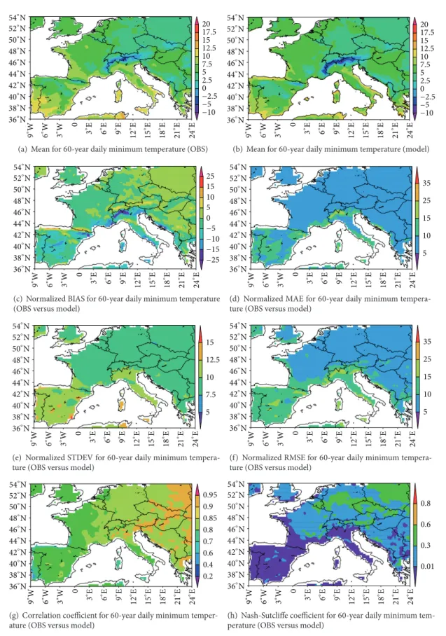
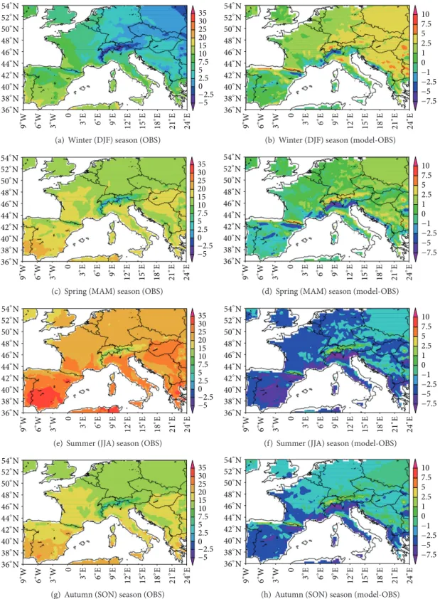
The 60-year mean seasonal mean temperatures from observations along with temperature difference between

model and observation values are presented in Figure 5.

The temperature differences indicate that model performance

is better in spring (Figures5(c)and5(d)) and autumn seasons

(Figures5(g)and5(h)) as compared to winter and summer

seasons where extreme conditions usually prevail. The mean

winter temperatures (Figures5(a)and5(b)) indicate a warm

Bias of 2.5 to 5∘C over Central and Eastern Europe and slight

warm bias of 1 to 2.5∘C over northern Europe, Mediterranean

region, and Iberia. Over Alps and limited areas in Iberia

model simulated a cold bias of −1 to 2.5∘C. The above

results indicate the model performs better over Iberia and Mediterranean region for winter mean temperatures. In

summer season (Figures5(e)and5(f)) the model produces a

cold bias in mean temperatures over most parts in Europe. It

produced a cold bias of−1 to −2.5∘C over northeastern Europe

and−2.5 to −5∘C over western and northern Europe and Italy.

An extreme cold bias of−7.5∘C is simulated over Alps and

southern Iberia. Similarly a cold bias of−1∘C over

northeast-ern and southeastnortheast-ern Europe,−1 to −2.5∘C over northern and

central Europe, and−2.5 to −5∘C over Iberia is simulated in

autumn season. The bias in the mean temperatures is of the

order of−1 to 1∘C over the entire domain in spring except Alps

and limited areas in Iberia where a cold bias of−2.5∘C is

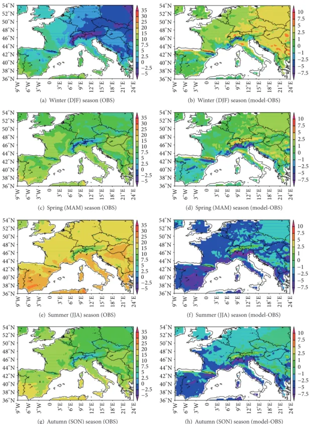
sim-ulated. Although the spatial seasonal temperature patterns generally agree well with observation patterns, the contours indicate clear cold bias in summer and autumn seasons and warm bias in winter season which indicates that the model generates relatively more errors in simulating the extremities of temperature common to winter and summer seasons than in the other two seasons. Hence, the maximum and minimum temperatures are analyzed in detail to obtain further insight. The seasonal mean of maximum temperatures in different

seasons (Figure 6) shows the model simulates a warm bias

(2.5 to 5∘C) in winter maximum temperatures (Figures6(a)

and 6(b)) over northeastern, Central, and Eastern Europe

and slight warm bias in Western Europe. In summer the

model produced a cold bias (−2.5 to −5∘C) (Figures 6(e)

and 6(f)) over most parts of the domain particularly over

Iberian region, Mediterranean and central northern Europe, and southeastern parts of Europe. In both spring and autumn seasons maximum temperatures are simulated in better agreement with corresponding observation means although with a slight cold bias in autumn and warm bias in spring. Thus, temperature simulation in both summer and winter is relatively poor as compared to the remaining two seasons

(Figures6(c),6(d),6(g), and6(h)). Nevertheless, the spatial

distribution patterns of mean seasonal temperatures are noted to follow observation pattern. The relatively poor performance for temperatures in summer and winter seasons could be due to deficiencies in the model surface physics

−5 −2.5 0 2.5 5 7.5 10 15 20 30 35 25 54∘_N 52∘_N 48∘N 46∘_N 44∘_N 42∘N 40∘N 50∘N 38∘_N 36∘_N 9 ∘W ∘₆W ∘₃W 0 ∘3E ∘6E ∘E9 ∘₁₂E ∘₁₅E ∘₁₈E ∘₂₁E ∘ ₂₄E

(a) Winter (DJF) season (OBS)

−5 −1 −2.5 −7.5 0 2.5 1 5 7.5 10 54∘N 52∘N 48∘_N 46∘N 44∘N 42∘_N 40∘_N 50∘_N 38∘N 36∘N 9 ∘ W ∘ ₆W ∘ ₃W 0 ∘ 3E ∘ 6E ∘ E9 ∘ ₁₂E ∘₁₅E ∘₁₈E ∘₂₁E ∘₂₄E

(b) Winter (DJF) season (model-OBS)

54∘N 52∘_N 48∘N 46∘N 44∘_N 42∘_N 40∘N 50∘_N 38∘N 36∘_N 9 ∘W ∘₆W ∘₃W 0 ∘₃E ∘₆E ∘E₉ ∘₁₂E ∘₁₅E ∘₁₈E ∘₂₁E ∘ ₂₄E −5 −2.5 0 2.5 5 7.5 10 15 20 30 35 25

(c) Spring (MAM) season (OBS)

54∘_N 52∘N 48∘_N 46∘_N 44∘N 42∘N 40∘_N 50∘N 38∘N 36∘N 9 ∘ W ∘ ₆W ∘ ₃W 0 ∘ ₃E ∘ ₆E ∘ E₉ ∘ ₁₂E ∘₁₅E ∘₁₈E ∘₂₁E ∘₂₄E −5 −1 −2.5 −7.5 0 2.5 1 5 7.5 10

(d) Spring (MAM) season (model-OBS)

54∘_N 52∘N 48∘_N 46∘_N 44∘N 42∘N 40∘_N 50∘N 38∘N 36∘N 9 ∘W ∘₆W ∘₃W 0 ∘3E ∘ 6E ∘ E9 ∘ ₁₂E ∘ ₁₅E ∘ ₁₈E ∘ ₂₁E ∘ ₂₄E −5 −2.5 0 2.5 5 7.5 10 15 20 30 35 25

(e) Summer (JJA) season (OBS)

54∘_N 52∘N 48∘N 46∘_N 44∘N 42∘N 40∘_N 50∘N 38∘_N 36∘_N 9 ∘W ∘₆W ∘₃W 0 ∘ 3E ∘ 6E ∘ E9 ∘ ₁₂E ∘ ₁₅E ∘ ₁₈E ∘ ₂₁E ∘ ₂₄E −5 −1 −2.5 −7.5 0 2.5 1 5 7.5 10

(f) Summer (JJA) season (model-OBS)

54∘N 52∘_N 48∘N 46∘_N 44∘_N 42∘N 40∘N 50∘N 38∘_N 36∘_N 9 ∘W ∘₆W ∘₃W 0 ∘3E ∘ 6E ∘ E9 ∘ ₁₂E ∘ ₁₅E ∘ ₁₈E ∘ ₂₁E ∘ ₂₄E −5 −2.5 0 2.5 5 7.5 10 15 20 30 35 25

(g) Autumn (SON) season (OBS)

54∘_N 52∘_N 48∘N 46∘_N 44∘_N 42∘N 40∘N 50∘N 38∘_N 36∘_N 9 ∘ W ∘ ₆W ∘₃W 0 ∘3E ∘6E ∘E9 ∘₁₂E ∘₁₅E ∘₁₈E ∘₂₁E ∘₂₄E −5 −1 −2.5 −7.5 0 2.5 1 5 7.5 10

(h) Autumn (SON) season (model-OBS)

Figure 5: 60-year mean seasonal mean temperatures at 2 m height (left panel from OBS and right panel from model-OBS). (a) and (b) for winter season (DJF); (c) and (d) for spring season (MAM); (e) and (f) for summer season (JJA); and (g) and (h) for autumn season (SON).

−5 −2.5 0 2.5 5 7.5 10 15 20 30 35 25 54∘N 52∘N 48∘_N 46∘N 44∘N 42∘_N 40∘_N 50∘_N 38∘N 36∘N 9 ∘ W ∘ ₆W ∘ ₃W 0 ∘3E ∘6E ∘E9 ∘₁₂E ∘₁₅E ∘₁₈E ∘₂₁E ∘₂₄E

(a) Winter (DJF) season (OBS)

−5 −1 −2.5 −7.5 0 2.5 1 5 7.5 10 54∘N 52∘N 48∘_N 46∘N 44∘N 42∘_N 40∘_N 50∘_N 38∘N 36∘N 9 ∘W ∘₆W ∘₃W 0 ∘ 3E ∘ 6E ∘ E9 ∘ ₁₂E ∘ ₁₅E ∘ ₁₈E ∘ ₂₁E ∘₂₄E

(b) Winter (DJF) season (model-OBS)

54∘_N 52∘_N 48∘N 46∘_N 44∘_N 42∘N 40∘N 50∘N 38∘_N 36∘_N 9 ∘ W ∘ ₆W ∘ ₃W 0 ∘ 3E ∘ 6E ∘ E9 ∘ ₁₂E ∘ ₁₅E ∘₁₈E ∘₂₁E ∘₂₄E −5 −2.5 0 2.5 5 7.5 10 15 20 30 35 25

(c) Spring (MAM) season (OBS)

54∘_N 52∘_N 48∘N 46∘_N 44∘_N 42∘N 40∘N 50∘N 38∘_N 36∘N 9 ∘W ∘₆W ∘₃W 0 ∘3E ∘6E ∘E9 ∘₁₂E ∘₁₅E ∘₁₈E ∘ ₂₁E ∘ ₂₄E −5 −1 −2.5 −7.5 0 2.5 1 5 7.5 10

(d) Spring (MAM) season (model-OBS)

54∘_N 52∘N 48∘_N 46∘N 44∘N 42∘_N 40∘_N 50∘N 38∘N 36∘N 9 ∘ W ∘ ₆W ∘ ₃W 0 ∘3E ∘6E ∘E9 ∘₁₂E ∘₁₅E ∘₁₈E ∘₂₁E ∘₂₄E −5 −2.5 0 2.5 5 7.5 10 15 20 30 35 25

(e) Summer (JJA) season (OBS)

54∘_N 52∘N 48∘_N 46∘N 44∘N 42∘_N 40∘_N 50∘N 38∘N 36∘N 9 ∘W ∘₆W ∘₃W 0 ∘ 3E ∘ 6E ∘ E9 ∘ ₁₂E ∘ ₁₅E ∘ ₁₈E ∘ ₂₁E ∘ ₂₄E −5 −1 −2.5 −7.5 0 2.5 1 5 7.5 10

(f) Summer (JJA) season (model-OBS)

54∘N 52∘N 48∘_N 46∘N 44∘N 42∘_N 40∘_N 50∘_N 38∘N 36∘N 9 ∘ W ∘ ₆W ∘ ₃W 0 ∘3E ∘6E ∘E9 ∘₁₂E ∘₁₅E ∘₁₈E ∘₂₁E ∘₂₄E −5 −2.5 0 2.5 5 7.5 10 15 20 30 35 25

(g) Autumn (SON) season (OBS)

54∘_N 52∘N 48∘_N 46∘N 44∘N 42∘_N 40∘N 50∘_N 38∘N 36∘_N 9 ∘W ∘₆W ∘₃W 0 ∘ 3E ∘ 6E ∘ E9 ∘ ₁₂E ∘ ₁₅E ∘ ₁₈E ∘ ₂₁E ∘ ₂₄E −5 −1 −2.5 −7.5 0 2.5 1 5 7.5 10

(h) Autumn (SON) season (model-OBS)

Figure 6: 60-year mean seasonal maximum temperatures at 2 m height (left panel from OBS and right panel from model-OBS). (a) and (b) for winter season (DJF); (c) and (d) for spring season (MAM); (e) and (f) for summer season (JJA); and (g) and (h) for autumn season (SON).

54N 52∘_N 48∘N 46∘N 44∘_N 42∘_N 40∘N 50∘_N 38∘N 36∘_N 9 ∘ W ∘ ₆W ∘ ₃W 0 ∘ 3E ∘ 6E ∘ E9 ∘ ₁₂E ∘ ₁₅E ∘₁₈E ∘₂₁E ∘₂₄E −5 −2.5 0 2.5 5 7.5 10 15 20 30 35 25

(a) Winter (DJF) season (OBS)

54N 52∘N 48∘_N 46∘_N 44∘N 42∘N 40∘_N 50∘N 38∘_N 36∘N 9 ∘W ∘₆W ∘₃W 0 ∘3E ∘6E ∘E9 ∘₁₂E ∘₁₅E ∘₁₈E ∘ ₂₁E ∘ ₂₄E −5 −1 −2.5 −7.5 0 2.5 1 5 7.5 10

(b) Winter (DJF) season (model-OBS)

54∘_N 52∘N 48∘_N 46∘N 44∘N 42∘_N 40∘N 50∘_N 38∘N 36∘_N 9 ∘ W ∘ ₆W ∘ ₃W 0 ∘3E ∘6E ∘E9 ∘₁₂E ∘₁₅E ∘₁₈E ∘₂₁E ∘₂₄E −5 −2.5 0 2.5 5 7.5 10 15 20 30 35 25

(c) Spring (MAM) season (OBS)

54∘N 52∘N 48∘_N 46∘N 44∘N 42∘_N 40∘N 50∘_N 38∘N 36∘_N 9 ∘ W ∘ ₆W ∘₃W 0 ∘3E ∘6E ∘E9 ∘₁₂E ∘₁₅E ∘₁₈E ∘₂₁E ∘₂₄E −5 −1 −2.5 −7.5 0 2.5 1 5 7.5 10

(d) Spring (MAM) season (model-OBS)

54∘_N 52∘N 48∘_N 46∘N 44∘N 42∘N 40∘_N 50∘_N 38∘_N 36∘N 9 ∘W ∘₆W ∘₃W 0 ∘3E ∘6E ∘E9 ∘₁₂E ∘₁₅E ∘₁₈E ∘₂₁E ∘ ₂₄E −5 −2.5 0 2.5 5 7.5 10 15 20 30 35 25

(e) Summer (JJA) season (OBS)

54∘_N 52∘_N 48∘N 46∘N 44∘_N 42∘_N 40∘N 50∘_N 38∘N 36∘_N 9 ∘W ∘₆W ∘₃W 0 ∘3E ∘6E ∘E9 ∘₁₂E ∘₁₅E ∘₁₈E ∘ ₂₁E ∘ ₂₄E −5 −1 −2.5 −7.5 0 2.5 1 5 7.5 10

(f) Summer (JJA) season (model-OBS)

54∘N 52∘N 48∘_N 46∘N 44∘N 42∘_N 40∘_N 50∘_N 38∘N 36∘N 9 ∘ W ∘ ₆W ∘ ₃W 0 ∘ 3E ∘ 6E ∘ E9 ∘ ₁₂E ∘₁₅E ∘₁₈E ∘₂₁E ∘₂₄E −5 −2.5 0 2.5 5 7.5 10 15 20 30 35 25

(g) Autumn (SON) season (OBS)

54∘_N 52∘_N 48∘N 46∘_N 44∘_N 42∘N 40∘N 50∘N 38∘_N 36∘_N 9 ∘ W ∘ ₆W ∘ ₃W 0 ∘ 3E ∘ 6E ∘E9 ∘₁₂E ∘₁₅E ∘₁₈E ∘₂₁E ∘₂₄E −5 −1 −2.5 −7.5 0 2.5 1 5 7.5 10

(h) Autumn (SON) season (model-OBS)

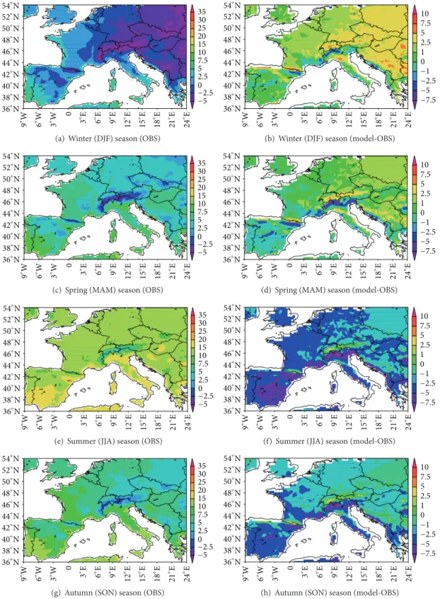
Figure 7: 60-year mean seasonal minimum temperatures at 2 m height (left panel from OBS and right panel from model-OBS). (a) and (b) for winter season (DJF); (c) and (d) for spring season (MAM); (e) and (f) for summer season (JJA); and (g) and (h) for autumn season (SON).

which is to be examined further considering the details of surface characteristics.

Figure 7 shows the mean seasonal minimum tempera-tures over different parts in Europe. Once again the results

show warm bias in winter minimum temperatures

(Fig-ures 7(a) and 7(b)) particularly over Eastern and Central

Europe, where the temperatures are simulated about 2 to

−15 −10 −25 −5 0 10 15 5 25 9 ∘ W ∘ ₆W 54∘N 52∘N 48∘_N 46∘_N 44∘N 42∘N 40∘_N 50∘N 38∘_N 36∘N 3 ∘ W 0 ∘3E ∘6E ∘9E ∘E₁₂ ∘₁₅E ∘₁₈E ∘₂₁E ∘₂₄E

(a) Normalized BIAS for summer maximum temperatures (OBS versus model)

54∘_N 52∘N 48∘_N 46∘N 44∘N 42∘_N 40∘N 50∘_N 38∘N 36∘_N 9 ∘W ∘₆W ∘₃W 0 ∘ 3E ∘ 6E ∘ E9 ∘ ₁₂E ∘ ₁₅E ∘ ₁₈E ∘ ₂₁E ∘ ₂₄E −15 −10 −25 −5 0 10 15 5 25

(b) Normalized BIAS for winter minimum temperatures (OBS versus model) 5 10 15 35 25 54∘_N 52∘N 48∘_N 46∘N 44∘N 42∘_N 40∘_N 50∘_N 38∘N 36∘N 9 ∘W ∘₆W ∘₃W 0 ∘3E ∘ 6E ∘ E9 ∘ ₁₂E ∘ ₁₅E ∘ ₁₈E ∘ ₂₁E ∘ ₂₄E

(c) Normalized MAE for summer maximum temperatures (OBS versus model)

54∘N 52∘_N 48∘N 46∘N 44∘_N 42∘N 40∘N 50∘_N 38∘_N 36∘_N 9 ∘W ∘₆W ∘₃W 0 ∘ 3E ∘ 6E ∘ E9 ∘ ₁₂E ∘ ₁₅E ∘ ₁₈E ∘ ₂₁E ∘ ₂₄E 5 10 15 35 25

(d) Normalized MAE for winter minimum temperatures (OBS versus model)

0.2 0.3 0.4 0.5 0.6 0.7 0.8 0.85 0.9 54∘N 52∘_N 48∘N 46∘N 44∘_N 42∘_N 40∘N 50∘_N 38∘N 36∘_N 9 ∘ W ∘ ₆W ∘ ₃W 0 ∘ 3E ∘ 6E ∘ E9 ∘ ₁₂E ∘₁₅E ∘₁₈E ∘₂₁E ∘₂₄E

(e) Correlation coefficient for summer maximum temperatures (OBS versus model)

54∘_N 52∘_N 48∘N 46∘N 44∘N 42∘N 40∘_N 50∘_N 38∘N 36∘_N 9 ∘ W ∘ ₆W ∘ ₃W 0 ∘3E ∘ 6E ∘E9 ∘ ₁₂E ∘ ₁₅E ∘₁₈E ∘₂₁E ∘₂₄E 0.2 0.3 0.4 0.5 0.6 0.7 0.8 0.850.9

(f) Correlation coefficient for winter minimum temperatures (OBS versus model)

5 10 15 25 35 54∘N 52∘_N 50∘N 48∘_N 46∘_N 44∘_N 42∘_N 40∘N 38∘_N 36∘N 9 ∘ W ∘ ₆W ∘₃W 0 ∘₃E ∘ ₆E ∘E₉ ∘ ₁₂E ∘₁₅E ∘₁₈E ∘₂₁E ∘₂₄E

(g) NSTDEV for summer maximum temperatures (OBS versus model) 54∘_N 52∘N 48∘_N 46∘_N 44∘N 42∘N 40∘_N 50∘N 38∘_N 36∘N 9 ∘W ∘₆W ∘₃W 0 ∘ ₃E ∘ ₆E ∘ E₉ ∘ ₁₂E ∘ ₁₅E ∘ ₁₈E ∘ ₂₁E ∘ ₂₄E 5 10 15 25 35

(h) NSTDEV for winter minimum temperatures (OBS versus model)

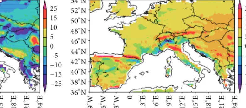
Figure 8: Statistical indices for 60-year summer seasonal maximum temperatures at 2 m height (left panel). Right panel is the same as left panel but for minimum temperatures in winter seasons from (a) and (b) for normalized BIAS (%); (c) and (d) for normalized MAE (%); (e) and (f) correlation coefficient and (g) and (h) are for NSTDEV (%) between observations and model.

0 2 4 6 8 10 1950 1960 1970 1980 1990 2000 E ven ts Year y = 0.0346x + 0.632 y = 0.0188x + 0.0113 CC= 0.3665 (a) Zone 1 0 2 4 6 8 10 1950 1960 1970 1980 1990 2000 E ven ts Year y = 0.0065x + 0.0842 CC= 0.202 y = 0.05x − 0.0904 (b) Zone 2 0 2 4 6 8 10 12 1950 1960 1970 1980 1990 2000 E ven ts Year y = 0.0487x + 0.6311 y = 0.0136x + 1.1339 CC= 0.461 (c) Zone 3 0 2 4 6 8 10 12 1950 1960 1970 1980 1990 2000 E ven ts Year y = 0.0545x + 0.3881 y = 0.0181x + 0.1316 CC= 0.445 (d) Zone 4 0 2 4 6 8 10 12 1950 1960 1970 1980 1990 2000 E ven ts Year y = 0.0532x + 0.1096 y = 0.0198x + 0.2475 CC= 0.681 (e) Zone 5 0 2 4 6 8 10 12 1950 1960 1970 1980 1990 2000 E ven ts Year y = 0.0421x + 0.7153 y = 0.0391x + 2.3226 CC= 0.694 (f) Zone 6 0 2 4 6 8 10 12 1950 1960 1970 1980 1990 2000 E ven ts Year y = 0.0408x + 0.8718 y = 0.0368x + 2.6621 CC= 0.701 (g) Zone 7 0 2 4 6 8 10 12 1950 1960 1970 1980 1990 2000 E ven ts Year y = 0.0311x + 1.2859 y = 0.0427x + 1.965 CC= 0.726 (h) Zone 8 0 2 4 6 8 10 12 1950 1960 1970 1980 1990 2000 E ven ts Year OBS Model y = 0.0487x + 0.8994 y = 0.0375x + 2.0559 CC= 0.656 (i) Zone 9 0 2 4 6 8 10 12 1950 1960 1970 1980 1990 2000 E ven ts Year OBS Model y = 0.0402x + 0.6729 CC= 0.378 y = −0.0128x + 2.2232 (j) Zone 10 Figure 9: Continued.

0 2 4 6 8 10 12 1950 1960 1970 1980 1990 2000 E ven ts Year y = 0.0311x + 0.7017 CC= 0.721 y = 0.0306x + 1.2994 (k) Zone 11 0 2 4 6 8 10 12 1950 1960 1970 1980 1990 2000 E ven ts Year y = 0.0426x + 0.5842 y = 0.0162x + 0.5226 CC= 0.626 (l) Zone 12 0 2 4 6 8 10 12 1950 1960 1970 1980 1990 2000 E ven ts Year y = 0.035x + 0.2322 CC= 0.678 y = 0.004x + 0.2621 (m) Zone 13 0 2 4 6 8 10 12 1950 1960 1970 1980 1990 2000 E ven ts Year y = 0.0304x + 0.222 y = 0.0072x + 0.1814 CC= 0.392 (n) Zone 14 0 2 4 6 8 10 12 1950 1960 1970 1980 1990 2000 E ven ts Year OBS Model y = 0.0403x + 0.3379 y = 0.0244x + 0.5051 CC= 0.601 (o) Zone 15

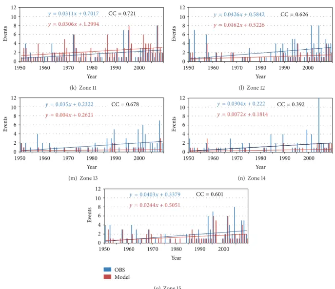
Figure 9: Time series for model and observed heat waves for all 15 zones along with their linear trends.

temperatures are simulated by about 5∘C lower than the

observations especially over western and Central Europe indicating a cold bias in summer minimum temperatures

(Figures 7(e) and 7(f)). In autumn season also there is

slight cold bias of−1 to −2.5∘C in minimum temperatures

over the whole of Europe. In spring season the simulated minimum temperatures fairly agree well with corresponding

values from observations (Figures7(c),7(d),7(g), and7(h))

in both patterns and with less bias values (−1 to 1∘_{C). The}

above results clearly demonstrate that model performance with respect to maximum temperatures in summer season and minimum temperatures in winter seasons is relatively poor as compared to the other two seasons. To quantify the errors, we computed different statistical indices NBIAS, NMAE, CC, and NSDEV for daily maximum temperatures in summer seasons and daily minimum temperatures in winter

seasons.Figure 8shows the NBIAS, NMAE, CC, and NSDEV.

The results indicate that for summer maximum temperatures

the NBIAS (Figure 8(a)) is about−25% in Iberian region,

−15% to 15% in western, central, and eastern parts of Europe,

and about 15% to 25% over Alps and a few areas in eastern Europe. This indicates underestimation of summer temper-atures in Iberian Peninsula and parts of western, central, and Eastern Europe and overestimation over Alps and other parts in Western Europe. The model in general produces a positive temperature bias during winter seasons over most parts of Europe (0 to 15%) with a higher positive bias (>15%) over Alps, coast line in Iberian Peninsula, central parts, Italy, and parts in western Europe. The above results indicate a warm bias in simulating winter minimum temperatures over almost the whole of Europe. Spatial error statistics clearly show the model performance is relatively poor over Iberia than the rest of Europe. The spatial distribution of NMAE confirms the poor performance of the model for winter minimum temperatures over Iberia, which is about 25%

in Iberian region (Figures8(c) and 8(d)) and less (10% to

15%) over Central and Eastern Europe. The NMAE in winter minimum temperatures is lower by 10% in all areas than the corresponding values for summer maximum temperatures indicating less bias in winter temperatures relative to summer.

Zones

Heat waves Cold waves

1950–2009 1950–1970 1971–2009 1950–2009 1950–1970 1971–2009

OBS MOD OBS MOD OBS MOD OBS MOD OBS MOD OBS MOD

1 105 35 29 5 77 31 27 27 0 8 27 19 2 86 17 11 1 75 16 59 17 18 5 41 12 3 127 93 32 28 96 67 50 18 18 6 32 12 4 123 41 29 9 96 34 47 33 15 12 32 21 5 104 51 14 10 90 41 36 15 13 7 23 8 6 120 211 27 55 94 160 97 63 25 9 72 54 7 127 227 29 64 99 168 110 59 30 13 80 46 8 134 196 34 50 102 150 138 55 33 11 105 44 9 143 192 33 52 110 143 107 57 23 12 84 45 10 114 110 31 45 83 70 87 31 16 9 71 22 11 99 134 25 38 74 98 165 82 30 20 135 62 12 113 61 28 19 85 42 109 49 37 13 72 36 13 78 23 17 6 61 17 99 68 48 34 51 34 14 69 24 15 8 54 16 46 23 24 13 22 10 15 94 75 25 21 69 54 79 47 18 12 61 35

Spatial correlations for summer and winter temperatures are computed at 95% significance level and are presented in

Figures8(e)and8(f). Spatial correlation distribution (Figures

8(e)and8(f)) shows high correlations (>0.6) for winter

indi-cating better simulation of winter minimum temperatures than the summer temperatures. In both the cases relatively poor correlations are found along the coastline of Iberia and a few isolated areas in Western Europe and Italy. Further

the spatial NSTDEV (Figures 8(g) and 8(h)) distributions

indicate higher model versus observation scatter (15–25) in summer as compared to the winter (5 to 10). The error

statistics (Figures 8(g) and 8(h)) indicate that the model

performance is poor over Iberian and Mediterranean regions relative to central and Eastern Europe. Overall, WRF-ARW model produces relatively better temperature simulation in the 60-year period in spring and autumn seasons than in summer and winter which is perhaps related to the representation of the land surface energy balance and the choice of surface physics used in the model. In general the model gives a cold bias in summer and warm bias in winter and the model performance is relatively better in Central and

Eastern Europe than in Iberian region. Garcia-Diez et al. [63]

have reported that the WRF model mean bias in temperature simulation significantly depends on the season, and warm bias in winter and cold bias in summer were simulated over Europe. Our present results corroborate their findings on a seasonal scale.

4.3. Extreme Heat and Cold Wave Occurrences. Here, the

changes in extreme weather events associated with heat waves in summers and cold waves in winters over different zones in Europe are presented. The model domain is divided into

15 zones based on topography (Figure 1). The frequency of

heat waves is derived from daily maximum temperatures in

summers and that of cold waves from the daily minimum temperatures in winter seasons. Occurrence of heat wave condition is defined from the number of instances with

maximum temperature exceeding 5∘C of its long-term mean

[61] consecutively over more than 3 days or more. Here the

long-term mean for summer maximum and winter minimum is computed from maximum daily temperatures for 60-year summer months and minimum daily temperatures for 60-year winter months, respectively. Similarly occurrence of cold wave condition is defined from the number of instances with

minimum temperature falling below 5∘C of its long-term

mean consecutively over 3 days or more. Daily minimum winter temperatures for the 60-year period are used with

deviation below 5∘C of its mean to identify the cold waves

over 60-year period.

Using the above criteria, we computed area averaged daily maximum temperatures from observations and model. The number of heat waves for each year in summer season is

computed and presented inFigure 9. Similarly area averaged

daily minimum temperatures are computed for all 60-year winter seasons and for each winter season the number of cold

wave events is identified (Figure 10). Linear curve fitting is

made and trend line between observed and modeled values of heat/cold waves are plotted to assess the trends in extreme temperature events.

It is seen that the number of simulated heat waves in most zones increases with time and the model simulated trends are consistent with the increasing trends found in observations except in zones 2, 10, 12, 13, and 14. It is noted that the number of heat wave (frequency) increases significantly in Central Europe especially in zones 6, 7, 8, 9, and 11, where the model produced more numbers of heat waves than the observed. Over zones 1 to 4 in Iberia, observations indicate significantly increasing number of heat waves in contrast to the model generated heat waves. The underrepresentation

0 2 4 6 8 10 1950 1960 1970 1980 1990 2000 E ven ts Year y = 0.0015x + 0.6051 y = 0.0018x + 0.3966 CC= 0.631 (a) Zone 1 0 2 4 6 8 10 1950 1960 1970 1980 1990 2000 E ven ts Year y = 0.0094x + 0.6977 y = −0.0024x + 0.3571 CC= 0.509 (b) Zone 2 0 2 4 6 8 10 1950 1960 1970 1980 1990 2000 E ven ts Year y = −0.0021x + 0.896 y = −0.0006x + 0.3186 CC= 0.517 (c) Zone 3 0 2 4 6 8 10 E ven ts 1950 1960 1970 1980 1990 2000 Year y = −0.0058x + 0.9605 y = −0.004x + 0.6712 CC = 0.620 (d) Zone 4 0 2 4 6 8 10 1950 1960 1970 1980 1990 2000 E ven ts Year y = −0.0042x + 0.7288 y = −0.0055x + 0.4169 CC= 0.569 (e) Zone 5 0 2 4 6 8 10 1950 1960 1970 1980 1990 2000 E ven ts Year y = 0.0206x + 0.9887 CC= 0.681 y = 0.0285x + 0.1814 (f) Zone 6 0 2 4 6 8 10 1950 1960 1970 1980 1990 2000 E ven ts Year y = 0.018x + 0.4333 CC= 0.423 y = 0.024x + 1.1028 (g) Zone 7 0 2 4 6 8 10 1950 1960 1970 1980 1990 2000 E ven ts Year y = 0.0374x + 1.1593 y = 0.0185x + 0.3531 CC= 0.467 (h) Zone 8 0 2 4 6 8 10 1950 1960 1970 1980 1990 2000 E ven ts Year OBS Model y = 0.0338x + 0.752 y = 0.0186x + 0.3831 CC= 0.36 (i) Zone 9 0 2 4 6 8 10 1950 1960 1970 1980 1990 2000 E ven ts Year OBS Model y = 0.0266x + 0.6373 y = 0.0053x + 0.3548 CC= 0.42 (j) Zone 10 Figure 10: Continued.

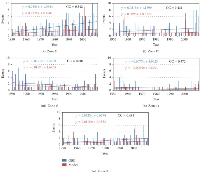
0 2 4 6 8 1950 1960 1970 1980 1990 2000 E ven ts Year y = 0.0553x + 1.0644 y = 0.0228x + 0.6701 CC= 0.342 (k) Zone 11 0 2 4 6 8 1950 1960 1970 1980 1990 2000 E ven ts Year y = 0.0215x + 1.1599 CC= 0.431 y = 0.0095x + 0.5277 (l) Zone 12 0 2 4 6 8 10 1950 1960 1970 1980 1990 2000 E ven ts Year y = −0.0251x + 2.4169 y = −0.0167x + 1.6435 CC= 0.601 (m) Zone 13 0 2 4 6 8 10 1950 1960 1970 1980 1990 2000 E ven ts Year y = −0.0077x + 1.0023 y = −0.0064x + 0.5791 CC= 0.372 (n) Zone 14 0 2 4 6 8 10 1950 1960 1970 1980 1990 2000 E ven ts Year OBS Model y = 0.0225x + 0.6294 y = 0.0115x + 0.4333 CC= 0.481 (o) Zone 15

Figure 10: Time series for model and observed cold waves for all 15 zones along with their linear trends.

in number of heat waves in zones 1–4 is consistent with the results obtained in the previous sections, where it was shown that the model exhibits a cold bias in simulating summer maximum temperatures over Iberian region and a few other parts. The correlations between model generated and observed heat waves for each zone are computed and

presented inFigure 9over each zone panel. Clearly the model

simulated good trends of heat wave simulation in most zones with remarkably high correlations (>0.6) except in zones 1–4, 10, and 14 where poor correlations of 0.22–0.45 are obtained. Similarly, the model simulated increasing number of cold waves in Central Europe and some parts of Eastern Europe

in zones 6 to 12 in agreement with observations (Figure 10).

Over Iberia (zones 1 to 5) no significant trend in cold waves is found. In zones 3–5, 13, and 14, located over Mediterranean region, a decreasing trend in cold waves is simulated as also found in observations though the trend is not very significant. Moderate correlations (∼0.34) in zone 11 and high correlations (0.68) in zone 6 are found for cold waves (Figure 10). In zone 2 located in Iberia (Figure 10) there is a

decreasing trend of cold waves in WRF while an increasing trend is noticed in observed ones. The number of heat waves and cold waves simulated and observed in different zones

is presented inTable 2. An increase in the number of heat

waves is noticed in all the zones during the period 1970–

2010 (Table 2) in both simulation and observations. More

than 80% of the total number of heat waves occurred during the period 1970–2010 in both observations and simulation. The incidence of heat waves as well as cold waves has been found to be highest in zones 6–12 followed by zones 15, 1, 4, and 3. In the remaining zones the heat and cold wave occurrence is not very significant. Thus the above analysis of frequency of heat waves and cold waves shows that both Central Europe and some parts of Eastern Europe are highly vulnerable to both heat waves and cold waves as significant linear increase is seen in the respective areas. The increasing trends in heat and cold wave events are well captured by model in agreement with observed extreme events. The most striking aspect is the inability of the model in simulating the heat waves in the Iberian region. In Iberia the model

−22.5 −17.5 −12.5 −7.5 −2.5 2.5 7.5 12.5 17.5 22.5 Zo n e 1 Zo n e 2 Zo n e 3 Zo n e 4 Zo n e 5 Zo n e 6 Zo n e 7 Zo n e 8 Zo n e 9 Zo n e 10 Zo n e 11 Zo n e 12 Zo n e 13 Zo n e 14 Zo n e 15 MAE Er ro rs ( %) STDEV BIAS

(a) Maximum temperatures in summer

0 2.5 5 7.5 10 12.5 15 Zo n e 1 Zo n e 2 Zo n e 3 Zo n e 4 Zo n e 5 Zo n e 6 Zo n e 7 Zo n e 8 Zo n e 9 Zo n e 10 Zo n e 11 Zo n e 12 Zo n e 13 Zo n e 14 Zo n e 15 Er ro rs ( %) MAE STDEV BIAS

(b) Minimum temperatures in winter seasons

Zo n e 1 Zo n e 2 Zo n e 3 Zo n e 4 Zo n e 5 Zo n e 6 Zo n e 7 Zo n e 8 Zo n e 9 Zo n e 10 Zo n e 11 Zo n e 12 Zo n e 13 Zo n e 14 Zo n e 15 0.6 0.650.7 0.750.8 0.850.9 Er ro rs ( %) Minimum temperatures Maximum temperatures (c) Correlation coefficient

Figure 11: Statistical indices (NBIAS, NSTDEV, and NMAE) between model and observed (a) maximum temperatures in summer, (b) minimum temperatures in winters and (c) correlation between model and observed maximum and minimum temperatures for each zone.

performed slightly better in cold waves simulation in terms of a high CC in zones 1 and 4 for the cold waves and the CC in the zones 1–4 are higher for cold waves than for heat waves. It is also noted that the cold waves in Mediterranean region are in decreasing trend though with less significance.

To examine the spatial variation of extreme heat and cold waves we analysed the daily maximum and minimum temperatures for summer and winter seasons averaged over different zones from observations and model. The statisti-cal metrics NBIAS, NSTDEV, NMAE, and CC computed between simulations and observations for maximum and minimum temperatures are computed and presented in

Figure 11. As already noted, the model underestimated sum-mer maximum temperatures indicating cold bias in all zones

with an error of−2.5 to −22.5%. The errors are less in Central

Europe, that is, from zones 6–13 and they are more (about 22.5%) in Iberian region. The same pattern is also noticed in NMAE. The NSTDEV indicates large scatter of the errors in the range of 10% to 12.5% and almost all zones exhibit similar scatter. Daily maximum temperatures for all 60-year summer seasons have correlations (>0.65), in that zone 11 has a maximum correlation of 0.79 followed by 0.78 in zone 10. For the minimum temperatures the NBIAS in different

zones is in the range of +2.5% to +12.5% which indicates a warm bias in all zones but the errors are lower in winter minimum temperatures than those in summer maximum temperatures. Zone 12 has the maximum warm bias followed by zones 15 and 11. In the remaining zones the errors are more or less similar and in zone 4 the errors are relatively low (about 2.5%). The NMAE and NSDEV in all zones are in the range of 7.5% to 12.5% and maximum NMAE and NSDEV are found in zone 11 followed by zone 15. The correlations for winter temperatures are improved (0.69–0.82) over summer maximum temperatures. The highest correlation (0.82) is noted in zone 10, followed by zone 6 with 0.81.

4.4. Long-Term Temperature Trends. To examine how the

model reproduced the long temperature trends in the study domain, we have made a time series analysis of spatial mean temperatures over (i) Iberian Peninsula, (ii) Central Europe, and (iii) Eastern Europe from values derived from model and

those from observations (Figure 12). From this Figure it is

evident that the deviations between observations and model values both in the seasonal maximum mean as well as min-imum mean values are high over Iberian Peninsula relative to Eastern and Central Europe regions. A simple linear trend analysis is performed to examine the temperature trends. This

20 10 0 −10 −20 Year 20 10 0 −10 −20 Year Te m pera tu re Te m pera tu re y = −6E − 05x + 15.619 R2_{= 0.0004} y = −4E − 05x + 13.31 R2_{= 0.0006 R}y = 6E − 05x + 10.5942_{= 0.0036} y = 0.0001x + 10.297_R2_{= 0.0064} Ju n 1, 50 Ju n 1, 52 Ju n 1, 54 Ju n 1, 56 Ju n 1, 58 Ju n 1, 60 Ju n 1, 62 Ju n 1, 64 Ju n 1, 66 Ju n 1, 68 Ju n 1, 70 Ja n 1, 71 Ja n 1, 73 Ja n 1, 75 Ja n 1, 77 Ja n 1, 79 Ja n 1, 81 Ja n 1, 83 Ja n 1, 85 Ja n 1, 87 Ja n 1, 89 Ja n 1, 91 Ja n 1, 93 Ja n 1, 95 Ja n 1, 97 Ja n 1, 99 Ja n 1, 01 Ja n 1, 03 Ja n 1, 05 Ja n 1, 07 Ja n 1, 09 (a) 30 20 10 0 −10 −20 Year 30 20 10 0 −10 −20 Year Te m pera tu re Te m pera tu re y = −5E − 05x + 11.592 R2_{= 0.0003} y = −9E − 05x + 11.34 R2_{= 0.0016} y = 8E − 05x + 7.3156_R2_{= 0.0041} y = 0.0001x + 7.0548_R2_{= 0.0052} Ju n 1, 50 Ju n 1, 52 Ju n 1, 54 Ju n 1, 56 Ju n 1, 58 Ju n 1, 60 Ju n 1, 62 Ju n 1, 64 Ju n 1, 66 Ju n 1, 68 Ju n 1, 70 Ja n 1, 71 Ja n 1, 73 Ja n 1, 75 Ja n 1, 77 Ja n 1, 79 Ja n 1, 81 Ja n 1, 83 Ja n 1, 85 Ja n 1, 87 Ja n 1, 89 Ja n 1, 91 Ja n 1, 93 Ja n 1, 95 Ja n 1, 97 Ja n 1, 99 Ja n 1, 01 Ja n 1, 03 Ja n 1, 05 Ja n 1, 07 Ja n 1, 09 (b) 30 20 10 0 −10 −20 Year 30 20 10 0 −10 −20 Year Te m pera tu re Te m pera tu re y = −7E − 05x + 9.1162 R2= 0.0003 y = −0.0002x + 12.723 R2_{= 0.0053} OBS Model OBS Model R2_{= 0.0021} y = 9E − 05x + 4.9467 R2= 0.0051 y = 0.0001x + 4.7919 Ju n 1, 50 Ju n 1, 52 Ju n 1, 54 Ju n 1, 56 Ju n 1, 58 Ju n 1, 60 Ju n 1, 62 Ju n 1, 64 Ju n 1, 66 Ju n 1, 68 Ju n 1, 70 Ja n 1, 71 Ja n 1, 73 Ja n 1, 75 Ja n 1, 77 Ja n 1, 79 Ja n 1, 81 Ja n 1, 83 Ja n 1, 85 Ja n 1, 87 Ja n 1, 89 Ja n 1, 91 Ja n 1, 93 Ja n 1, 95 Ja n 1, 97 Ja n 1, 99 Ja n 1, 01 Ja n 1, 03 Ja n 1, 05 Ja n 1, 07 Ja n 1, 09 (c)

Figure 12: Time series of model and observed daily mean temperatures (left panel is for the period of 1950–1970 and right panel is for 1971–2010) averaged over (a) Iberia, (b) Central Europe, and (c) Eastern Europe regions.

has already been noted in the spatial distribution of seasonal temperatures discussed above. In all the three regions there is a very small decreasing trend in mean temperatures in the period from 1950 to 1970 and a very small increasing trend in mean temperatures in the period from 1970 to 2010 though the variation is not very significant. Except for the Iberian Peninsula region the model is able to reproduce the peaks of temperature quite well throughout the period 1950–2010 in the rest of Europe. The trends in simulated temperature are noted to agree very well with observed temperatures.

5. Summary and Conclusion

A long-term regional climate simulation is performed over Europe using the WRF-ARW regional climate model by downscaling the NCEP reanalysis data at a 25 km model horizontal resolution. The model simulated mean, maximum, minimum, seasonal mean, maximum, and minimum tem-peratures are analysed by comparisons with corresponding data derived from E-OBS analysis data sets over the study domain. A comparison of the spatial patterns of the above