Cellular Automata
and
Cryptography
Tiago Santos
Dissertação de Mestrado apresentada à
Faculdade de Ciências da Universidade do Porto em Ciência de Computadores
Cellular Automata
and
Cryptography
Tiago Santos
Mestrado em Ciência de Computadores
Departamento de Ciências de Computadores 2014
Orientador
Prof. Rogério Reis, DCC
Coorientador
O Presidente do Júri,
This thesis gives an introduction to cellular automata and their applications in cryptog-raphy. We can find references to cryptographic techniques as far as the 1900 B.C.. Since then, cryptography has evolved and is now one of the cornerstones of our information society. From electronic payments to database security, passing through access control, messages authentication and corporative security, cryptography has become ubiquitous in our world. Historically speaking, the study of cellular automata is a very recent field of research. However its popularity has been steadily increasing, not only because of their ability to model complex dynamic systems, but also, due their inherent simplis-tic and high parallelizable structure. In this thesis, we start by introducing the basic concepts of cryptography and cellular automata, presenting some of the best examples of cryptographic systems with cellular automata as their main component. Then we focus our attention to one of the few public key systems based on cellular automata in existence, proposed by Kari. We analyze Kari’s proposal by giving a more detailed description. We also discuss an algorithm of this cryptosystem and provide some critics on its implementation and on its security.
Esta tese apresenta uma introdu¸c˜ao aos aut´omatos celulares e a sua aplica¸c˜ao `a criptogra-fia. Criptografia ´e uma ´area historicamente velha, existindo registos hist´oricos datados de 1900 B.C que a mencionam. Desde ent˜ao, a criptografia tornou-se num dos pilares da nossa sociedade da informa¸c˜ao. Devido `a sua importˆancia, a criptografia ´e neste momento ub´ıqua em v´arios dom´ınios, desde os pagamentos eletr´onicos `a seguran¸ca cor-porativa e de bases de dados, passando pelo controlo de acessos e assinaturas digitais. Historicamente falando, os automatos cellulares s˜ao ainda um campo de investiga¸c˜ao muito recente. No entando, a sua popularidade tem estado a crescer, n˜ao s´o devido `
as suas capacidades em modelar sistemas dinˆamicos complexos, mas tamb´em, devido `
a sua natureza simplista e estrutura altamente paraleliz´avel. Nesta tese, come¸camos por introduzir os conceitos b´asicos de criptografia e aut´omatos celulares, apresentando depois os melhores exemplos de aplica¸c˜oes de sistemas criptogr´aficos que utilizam os aut´omatos como um dos seus principais componentes. Depois focamos a nossa aten¸c˜ao para um sistema de chave p´ublica baseado em aut´omatos celulares, proposto por Kari. Analisamos este sistema e apresentamos-lo de uma forma detalhada. Finalizamos com a apresenta¸c˜ao e discuss˜ao de uma implementa¸c˜ao deste sistema, fornecendo cr´ıticas sobre o seu algoritmo e a sua seguran¸ca.
Foremost, I would like to express my sincere gratitude to my advisors Prof. Rog´erio Reis and Prof. Ant´onio Machiavelo for the continuous support of my MSc study and research, for their patience, motivation, enthusiasm, and immense knowledge. Their guidance helped me in all the time of research and writing of this thesis.
To all my professors that contributed to my academic formation.
To everybody, thank you.
Abstract v
Resumo vii
Acknowledgements ix
List of Figures xiii
List of Tables xv Abbreviations xvii 1 Introduction 1 1.1 Motivation . . . 1 1.2 Thesis outline . . . 2 2 Fundamentals of Cryptography 3 2.1 Cryptology . . . 3
2.2 The Importance of Cryptography . . . 4
2.3 Definition of a Cryptosystem . . . 5 2.4 Private-Key Cryptosystems . . . 6 2.5 Public-Key Cryptosystems . . . 8 2.6 Block Cipher . . . 10 2.7 Stream Ciphers . . . 10 2.8 Good Ciphers . . . 11
2.9 Cryptanalysis and Attacks . . . 12
3 Cellular Automata 15 3.1 Introduction . . . 15 3.1.1 Brief History . . . 15 3.1.2 Applications . . . 16 3.2 Formal Definition . . . 17 3.2.1 Cellular Automata . . . 17 3.2.2 Local Function . . . 17
3.2.3 Elementary Cellular Automata . . . 18
3.2.4 Global Function . . . 19
3.2.5 Neighborhoods . . . 20
3.2.6 Boundaries of Finite Latices . . . 22
3.2.7 Classification Systems . . . 22
3.3 Reversibility . . . 24
4 Brief Overview of Research on CA-based Cryptography 29 4.1 Pseudo Random Number Generators . . . 29
4.2 Block Encryption With Second-Order Cellular Automata . . . 33
4.3 Secret Sharing Schemes . . . 36
4.4 S-Boxes . . . 40 4.5 CA Attractors . . . 42 4.6 Hash Functions . . . 44 5 Kari’s Cryptosystem 47 5.1 Kari Proposal . . . 47 5.1.1 Self-Invertible Markers . . . 51
5.1.2 Public and Private Keys . . . 55
5.1.3 Encryption and Decryption . . . 60
5.1.4 Injectivity . . . 63
5.1.5 Number of Markers . . . 66
5.1.6 Public Key Size . . . 67
5.1.7 Safety Against Brute Force Attacks . . . 68
5.2 Clarridge and Salomaa Algorithm . . . 69
5.2.1 Definitions . . . 70
5.2.2 Neighborhood Size . . . 70
5.2.3 Examples . . . 73
5.2.4 Algorithm and Security Analysis . . . 76
6 Conclusions 81 A Clarridge and Salomaa Algorithm Implementation 83 A.1 Introduction . . . 83
A.2 Documentation . . . 83
A.3 Prerequisites . . . 84
A.4 Source Code . . . 84
A.5 Description . . . 86
2.1 The field of cryptology. . . 3
2.2 Unprotected communications. . . 4
2.3 Protected communications. . . 5
2.4 A generic cryptosystem. . . 6
2.5 Symmetric key operation. . . 7
2.6 The problem of the numbers of keys in symmetric key systems. . . 7
2.7 Asymmetric key operation. . . 8
2.8 Encryption and decryption operations. . . 11
3.1 All possible states configurations of the neighborhoods in any ECA. . . . 18
3.2 Orbits . . . 20
3.3 Example of a space-time diagram. . . 21
3.4 The two most common neighborhoods for two-dimensional CA with radius 2. 21 3.5 Three different types of boundaries. . . 22
3.6 Examples of space-time diagrams of the four Wolfram classes. . . 23
3.7 Examples of reversible cellular automata. . . 24
3.8 Simple CA explicitly set to be reversible . . . 26
3.9 Simple CA explicitly designed to be reversible. . . 26
3.10 Rule 30 and reversible rule 30R . . . 27
4.1 Structure of an additive PCA. . . 31
4.2 Simplified encryption and decryption process. . . 34
4.3 Single round of Bouvry’ system. . . 35
4.4 All basins of rule 60 applied to a one-dimensional CA of size 7. . . 43
5.1 Example of a marker. The gray square in the patterns represents the cell on which the marker is been applied to. . . 48
5.2 Marker operating on a cell. . . 50
5.3 Marker operating on another cell. . . 51
5.4 A reversible marker. . . 53
5.5 The effects of a reversible marker on a given configuration. . . 54
5.6 Another reversible marker. . . 54
5.7 A non-reversible marker. . . 55
5.8 The effects of a non-reversible marker on a given configuration. . . 55
5.9 A few entries in a hypothetical public key table. . . 56
5.10 Alternatives to M3. . . 60
5.11 Encryption using the public key. . . 61
5.12 A set of reversible markers. . . 61
5.13 Creating the entries of the public key. . . 62
5.14 Encryption of a plaintext using the public key. . . 62
5.15 Decryption of the ciphertext. . . 63
5.16 Two 1-dimensional reversible markers. . . 68
2.1 Required times for brute force attacks. . . 14 5.1 Number of distinct markers depending on the number of states and
neigh-borhood size. . . 67 5.2 Number of distinct markers generated by the algorithm. . . 78 5.3 Number of available sets of markers. . . 79
AES Advanced Encryption Standard CA Cellular Automata
DES Data Encryption Standard ECA Elementary Cellular Automata
FDM CA Fixed Domain Marker Cellular Automaton ICA Invertible Cellular Automata
IDEA International Data Encryption Algorithm KDC Key Distribution Center
LCA Linear Cellular Automata LFSR Linear Feedback Shift Register LMCA Linear Memory Cellular Automata MCA Memory Cellular Automata
PCA Programmable Cellular Automata PGP Pretty Good Privacy
PRNG Pseudo Random Number Generator RCA Reversible Cellular Automata
Introduction
1.1
Motivation
Due the ubiquity of digital communications and digital data in today’s world, the devel-opment of techniques and tools to protect them have become increasingly more impor-tant. This required protection encompasses a set of requirements and solutions where cryptography is a primary pillar. Among the cryptographic goals we find secrecy, au-thenticity and preservation of the integrity of the data that it is protecting. We can split cryptographic systems in two groups: symmetric-key and public-key systems. In the first group, the same key is used both for encryption and the decryption. In the second, encryption and decryption are done using different keys.
Cellular automata (CA) is a decentralized computing model capable of providing a platform for performing complex computations using only local information. They are composed by a number of components, called cells, with local connectivity. Each cell is at one state at a time and its temporal change follows a simple transition rule that depends on both the current state and on the states of its neighboring cells.
Despite its simple structure, cellular automata can be as expressive as Turing machines [TM90]. Due to their capacity of executing complex computations with high efficiency and robustness, they can be a very useful tool for simulating the behavior of complex systems. They have been the subject of rigorous mathematical analysis and their ap-plications have extended into a myriad of fields, such as, simulations of gas behavior,
percolation processes and forest fire propagation, in the conception of massive parallel computers and in the study of urban development. Together with its easy implemen-tation in parallel architectures, cellular automata have become a very interesting and efficient tool in the cryptographic field. However they have been mainly employed in symmetric key cryptosystem.
The main goal of this thesis is to explore how cellular automata have been used in cryp-tography, and therefore we start by exposing the most relevant cryptosystems that make use of cellular automata, including pseudo-random generators, secret sharing schemes, S-Boxes, hash functions and others. Because of both the scarcity of CA-based public key systems and the lack of a good description of these systems, we have dedicated an entire chapter to a particular system and to an implementation of it. Our main goal is to attempt to provide a more clear and detailed description of it.
1.2
Thesis outline
The thesis is organized as follows. We start by introducing the basic concepts of cryp-tography in chapter 2, presenting its goals, systems and main characteristics.
In chapter 3, we present a brief introduction to CA, the history, formal definitions, main characteristics, applications and classification.
Chapter 4 displays an overview of the most relevant cryptosystems and works on cryp-tography that uses CA as their main component.
In chapter 5, we present and discuss Kari’s CA-based public key cryptosystem and an algorithm for its implementation.
Finally, chapter 6 ends the thesis with a short conclusion and a presentation of a road-map for future research.
Fundamentals of Cryptography
2.1
Cryptology
Cryptology is a very broad term. It encompasses both the study of techniques related to all aspects of data security as well the study of the principles and methods of trans-forming one message into another (see figure 2.1). We can say, cryptology is the science and study of cryptanalysis and cryptography.
Figure 2.1: The field of cryptology.
Cryptography is a crucial part of any secure communication. The need of security and privacy in communications has been an essential necessity since antiquity, with references dating back as far as 1900 B.C. [WM07]. It has extended far beyond its initial application in communications. Now we see cryptography in countless areas, from database content protection to communications authentication.
Despite its age, most modern cryptographic techniques are based on advances made in the past few decades. Singh’s book [Sin00] provides a fascinating look at the long history of encryption and its applications. Extensive overviews on cryptographic systems can be found in many classical works by authors as Schneier [Sch95], Stallings [Sta11] and Menezes [MVO96].
2.2
The Importance of Cryptography
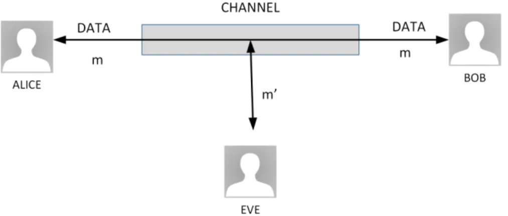
Two communicating entities, which we will call Alice and Bob, want to communicate with each other securely. As examples of such entities we find web browser/server for electronic transactions, on-line banking client/server, DNS servers or routers exchanging routing table updates. Another entity, Eve, acts as an intruder with the goal of interfer-ing with the communication between Alice and Bob. Among her goals we find message modification, connection hijack and impersonation, among others.
Consider the following security risks that Alice and Bob can face when communicating in an unprotected channel, as illustrate in figure 2.2.
If Eve intercepts and understands all secret messages by eavesdropping on the commu-nication, then we have loss of privacy and confidentiality.
On the other hand, if Eve is able to modify the message while in transit, and if either Bob or Alice are unable to detect this, then we have loss of integrity.
If Eve sends messages to Bob, by pretending to be Alice, and Bob is unable to verify the source of the information then we lack authentication.
Both Bob and Alice can also repudiate any message sent by each other.
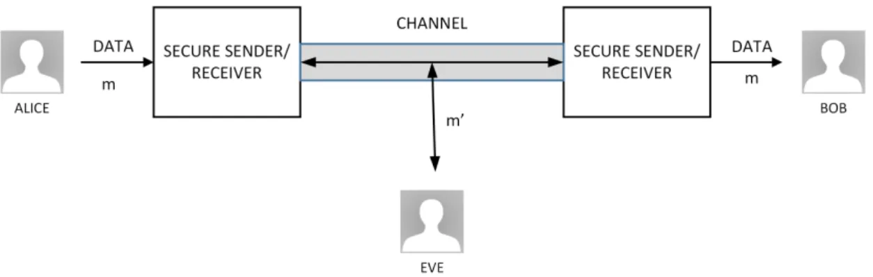
From all the above, we can see that security must be used on both sides of the commu-nication channel. The solution for these problems passes by the use of cryptography to secure the channel and the data (see figure 2.3).
Figure 2.3: Protected communications.
We are now able to identify the following cryptographic goals [MVO96]: confidentiality, data integrity, authenticity and non-repudiation. Confidentiality or privacy keeps the contents of a message secret from all non-authorized third-parties. Integrity deals with the non-authorized alteration of data, including insertion, substitution and deletion. Authenticity deals with the identification of the message, its origins. Non-repudiation prevents an entity from denying previous actions or commitments.
2.3
Definition of a Cryptosystem
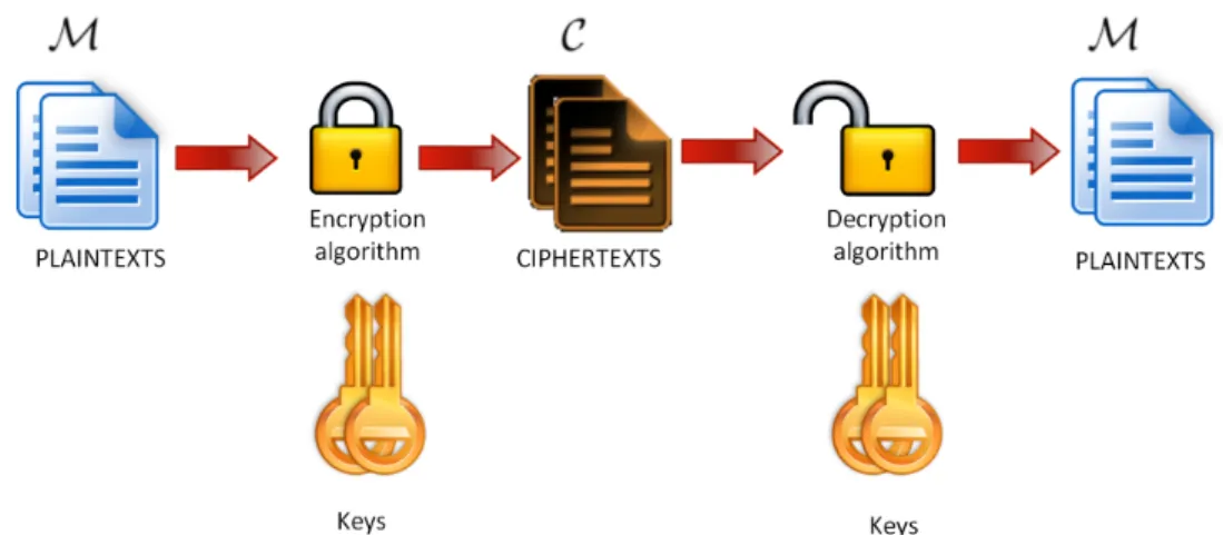
When can define a cryptosystem as a five-tuple (M, C, K, E , D), where M is a finite set of plaintexts (original messages), C a finite set of ciphertexts (coded messages), K a finite set of keys (keyspace), E a finite set of enciphering transformations ek1 : M → C and
D a finite set of deciphering transformations dk2 : C → M. For each key k1 ∈ K there
is an encryption transformation ek1 ∈ E and a corresponding decryption transformation
dk2 ∈ D. Also, for each ek1 and dk2 : dk2(ek1(m)) = m, ∀m ∈ M.
A representation of a generic cryptosystem can be seen in figure 2.4.
Figure 2.4: A generic cryptosystem.
A cryptosystem can be characterized according to:
• The type of operations used in the transformation of the plaintext into ciphertext. • Number of keys used, usually single key for private or symmetric systems and
two-key for public or asymmetric systems.
• How the plaintext is processed: block or stream cipher.
2.4
Private-Key Cryptosystems
In these type of cryptosystems, all communicating parties share a common secret key, k1 = k2 = k, which is used both for the encryption and the decryption operations (see figure 2.5).
There are hundreds if not thousands of symmetric key algorithms. Examples include the Data Encryption Standard (DES) [NBoS77], the International Data Encryption Standard (IDEA) [Lai92], the Advanced Encryption Standard (AES) [PT01], the RC5 [Riv94] and the RC6 [RRSY].
Figure 2.5: Symmetric key operation.
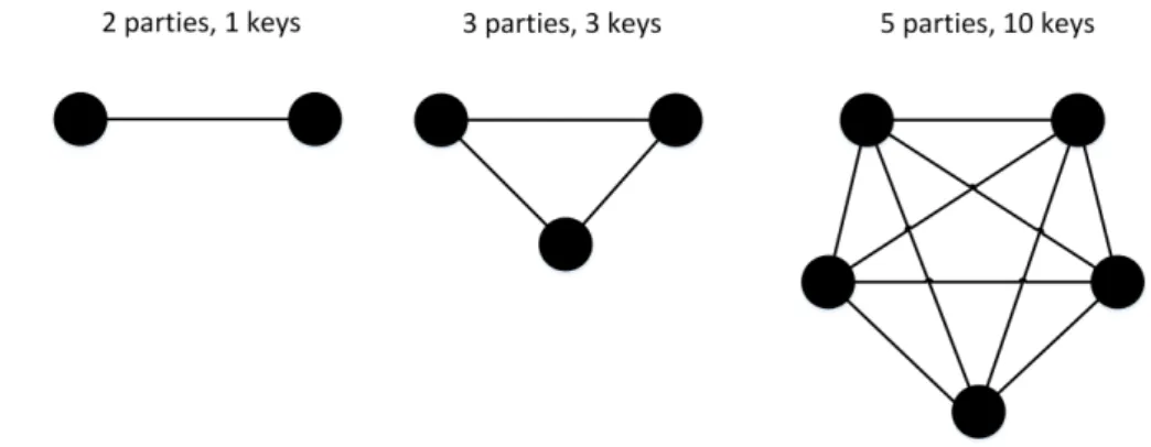
Symmetric key systems are much faster than public key cryptography, in the order of 1000 to 10000 faster, and even faster if they are implemented with dedicated hardware. Despite their good performance and security, they do have some significant downsides. A serious problem is the key management problem. This issue appears even in small-scale networks. As the number of users increases, the number of keys required to provide secure communications exhibit a quadratic growth. For example, a network of N users requires at least N (N − 1)/2 keys and in this case each user would need to keep N − 1 keys in secret. As we can observe in figure 2.6, both the numbers of keys and the number of secure channels to distribute the keys rapidly starts to increase with the number of users. There is also the necessity for a secure channel for the exchange of the secret
Figure 2.6: The problem of the numbers of keys in symmetric key systems.
key. To solve this issue, Deffie-Hellman methods or a trusted key distribution center (KDC) acting as intermediary between entities are used. Also if a single secret key is shared between N users, then it requires only one to betray the secret to compromise all communications. Since both parties share the same key, there are also problems with the authenticity of a message.
We can see that there are four requirements for the secure use of symmetric encryption: a strong encryption algorithm, a secret key known only to sender / receiver, always assume that the encryption algorithm is known and a secure channel to distribute key.
2.5
Public-Key Cryptosystems
Public key or asymmetric systems were developed to address two key issues: how to have secure communications without having to trust a KDC with the key and how to verify if a message comes intact from the claimed sender (digital signatures).
The idea of public-key cryptosystems was proposed by Diffie, Hellman [DH76] and Merkle. They demonstrated the principle with their Diffie-Hellman Key Exchange al-gorithm, which revealed to be a radically different and elegant approach for secure communications. Since this milestone, several others algorithms have emerged, such as RSA [RSA78]), Merkle-Hellman [MH78], El Gamal [Elg85] and Elliptic curves [Lan05], all of them still in use today.
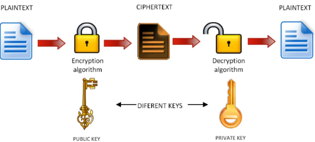
In public key cryptography keys are created in related pairs, one for encryption and a different one for decryption, k16= k2, a public key and a private key (see figure 2.7). The
Figure 2.7: Asymmetric key operation.
public-key can be freely published without compromising the private one, which can also be known by anybody, and can be used to encrypt messages and to verify signatures A private key, which should be kept in secret, should only be known to the recipient, and it is used both to decrypt messages and to sign or create signatures.
Public key algorithms are based on mathematical functions. Furthermore the public and the private keys are related in such a way that even with the knowledge of the public key, it is virtually impossible to deduce the private key. Therefore, these cryp-tosystems depend on the existence of one-way functions. Despite the fact that there are no evidences on the existence of such functions, we can speculate their existence, by considering some assumptions about their complexity to be true. Examples of such functions include multiplication/factorization and exponentiation/logarithms. The key point is to find a trap door in these function so that it becomes relatively easy to find their inverse given some knowledge.
Public key systems present then three main characteristics:
• It is computationally infeasible to find the decryption key knowing only the algo-rithm and the encryption key.
• It is computationally easy to encrypt and decrypt messages when the respective key is known.
Because public key systems requires the use of very large numbers and expensive mathe-matical operations, these systems are slow when compared with symmetric key schemes. Generally, encrypting large messages using public key systems can be considered imprac-tical. Therefore, public key cryptography should be considered a complement rather than a replacement of the private key cryptography: use a public key cipher (such as RSA) to distribute keys and use a private key cipher (such as DES) to encrypt and decrypt messages.
Deterministic public-key systems are susceptible to dictionary attacks. But, if public key systems are used only to encrypt small messages, such as keys, these types of attacks are not a practical problem. The most significant attack against these systems is the man-in-the-middle attack. In this attack, Eve intercepts messages sent by Bob to Alice or by Alice to Bob. Since Eve knows the public keys of both Alice and Bob, all she needs is to hijack the communication channel between Alice and Bob during the exchange of their public key, by sending her public key instead of theirs. Now Eve can intercept and read every message between Alice and Bob and even changing them in transit.
There are however several misconceptions about public key encryption. Among them, we can find the following two: the public key encryption is more secure than symmetric
key encryption and public key encryption is a general purpose technique that has made symmetric encryption obsolete. Since the security of any good encryption scheme de-pends on the length of the key and on the computational resources required to break the cipher, there are no major differences between the two systems. Also, due to the higher computational requirements of current public key systems when compared to the symmetric ones, conventional encryption will continue to be used in the foreseeable future.
2.6
Block Cipher
Block ciphers splits the plaintext into blocks of fixed length, and the encryption is executed on one block at a time. Typical block sizes are 64 bits or 128 bits and messages are padded (with extra bits) to fit the block size. In mathematical terms we have the plaintext ¯M → ¯M = m1, m2, ..., mn, where mi represents a block and the corresponding encrypted text given by ¯C = c2, ..., cn, with ci = ek(mi) and k fixed.
The encryption function ek requires a complex operation. To achieve the desired level of complexity all block ciphers are iterative algorithms where the data passes through multiples rounds of one or more simple operations, such as, permutations and shifts. Examples of block ciphers includes DES and IDEA. There are several factors that in-fluence the security of a symmetric block cipher, such as, the quality of the algorithm and the length of the key (e.g., 64 bit blocks are questionable, but 128 bit blocks are considered more than adequate). Therefore designers of cryptographic systems should consider a trade-off between efficiency and security.
Block ciphers can operate in one of several modes [MVO96], been the four most common the Electronic Codebook Book (ECB), the Cipher Block Chaining (CBC), the Cipher FeedBack (CFB) and the Output FeedBack (OFB).
2.7
Stream Ciphers
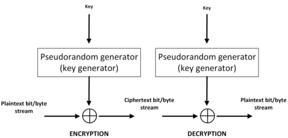
In stream ciphers the encryption of the plain text is performed at the bit or byte level, i.e., individual bits/characters of plaintext are encrypted immediately into bits/characters
of ciphertext, as illustrate in figure 2.8.
Figure 2.8: Encryption and decryption operations.
Mathematically speaking, we have c1, c2, ..., cn = es1(m1), es2(m2), ..., esn(mn), where
s1, s2, ..., snis the key stream. The encryption function esi is a simple operation, usually
a simple XOR. The key component of these ciphers lies in the generation of the key stream.
Stream cipher are similar to one-time pad cipher [Kah96], but with a pseudo-random key instead of random key. The randomness of the stream key completely destroys any statistically properties in the message. The stream key should never be reuse, otherwise it would be possible to recover messages. Example of such ciphers includes the RC4.
2.8
Good Ciphers
The strength of any encryption method comes from the algorithm, secrecy of the key, length of the key, initialization vectors, and how all these elements work together. A cipher needs to obscure statistical properties of original message. In 1945 Shannon suggested two characteristics for thwarting cryptanalysis based upon statistical analysis: diffusion and confusion. Diffusion dissipates the statistical structure of plaintext into long-range statistics, i.e., the cipher should be able to spread the information from the plaintext over the entire ciphertext. This means that the interceptor needs access to a lot more ciphertext to infer the algorithm. The confusion property makes the relationship between ciphertext and key as complex as possible. This cause the interceptor not to be able to predict what changing one character in the plaintext does to the ciphertext.
In 1949, Shannon [Sha49] proposed five characteristics that a good cipher should exhibit:
1. The amount of secrecy required should determine the amount of labor appropriate for encryption/decryption, i.e., the more security, the more encryption.
2. The set of keys and enciphering algorithm should be free from complexity. 3. The implementation should be as simple as possible.
4. The errors in ciphering should not propagate and cause further corruption of the message. One error should not compromise the entire encryption process.
5. The size of the ciphertext should be no larger than the size of the plaintext
Because these criteria were developed before modern computers, some points are no longer a limitation. For example, the complexity of the cipher is no longer a main issue in today’s modern fast computers.
2.9
Cryptanalysis and Attacks
Cryptanalysis is the study of techniques to defeat cryptographic techniques. Its goal is to find weakness in ciphers, ciphertexts and cryptosystems, in order to recover the plaintext or any other useful information. It usually involves the detailed study on how the sys-tem works and in solving carefully constructed mathematical problems. Cryptanalysis usually excludes methods of attack that do not target weaknesses of the cryptographic system, e.g., using brute force against an algorithm without any knowledge of the algo-rithm.
We split attacks in two main classes: passive and active. Passive attacks includes eaves-dropping and network sniffing. They are passive because the attacker does not affect the cryptographic system, making it hard to detect. Active attacks include altering messages and system files and hijacking communications. It is called active because the attacker is actively affecting some aspect of the cryptographic protocol.
We can also classify attacks in another two classes: cryptanalytic attacks and imple-mentation attacks. While in cryptanalytic attacks the cryptanalyst attempts to attack
mathematical weakness in the algorithms, in the implementation attacks class the crypt-analyst focus his attack on the specific implementation of the cipher.
Depending on what a cryptanalyst has to work with, attacks can be classified into the following models, which can refer to either of the two above classes:
• Ciphertext only attack – the cryptanalyst has knowledge of some ciphertexts c1 = ek(m1), c2= ek(m2), ..., and his goal is to obtain m1, m2, or the key k.
• Known plaintext attack – the cryptanalyst knows some pairs (m1, c1= ek(m1)), (m2, c2 = ek(m2)), ..., and his ultimate goal is to obtain the key k.
• Chosen plaintext attack and Adaptive-chose plaintext attack – the cryptanalyst chooses the plaintext to be encrypted by the system and analyzes the resulting ci-phertext. In a adaptive-chosen plaintext attack, he can choose a message to be en-crypted based on previously achieved results. Hence, the cryptanalyst knows some pairs (m1, c1 = ek(m1)), (m2, c2 = ek(m2)), ..., of which he can choose m1, m2, ... and his goal is to obtain the key k. Often this attack implies that the cryptanalyst will attempt to feed a planned sequence of messages, in order to reveal the most about how the data is being encrypted.
• Chosen ciphertext attack and Adaptive-chosen ciphertext attack – In the chosen and adaptive-chosen ciphertext attacks, the cryptanalyst chooses a ciphertext and obtains the corresponding plaintext, therefore he can select ciphertexts based on previous results. He has some pairs (m1, c1 = ek(m1)), (m2, c2 = ek(m2)), ..., of which he can choose c1, c2, ..., and once again, his goal is to obtain the key k.
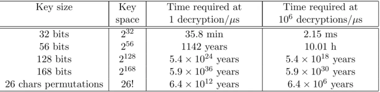
There are countless attack techniques, among which we can find side channel attack, brute force attacks, implementation exploitation and replay attacks. In side channel attacks, the cryptanalyst uses incidental information that can reveal important infor-mation about the key and plaintext, such as the sounds produced by keystrokes while the plaintext is typed. In a brute force attacks, the cryptanalyst performs an exhaustive search over the keyspace in hopes to find the right one. Cleary, this type of attack is expensive and time consuming. To give an idea on the time consuming of this type of attack, in table 2.1 we can observe the required times to perform an exhaustive search over different key spaces.
Key size Key space Time required at 1 decryption/µs Time required at 106 decryptions/µs 32 bits 232 35.8 min 2.15 ms 56 bits 256 1142 years 10.01 h
128 bits 2128 5.4 × 1024years 5.4 × 10¹⁸years 168 bits 2168 5.9 × 1036years 5.9 × 1030years 26 chars permutations 26! 6.4 × 10¹²years 6.4 × 10⁶ years
Table 2.1: Required times for brute force attacks.
Perhaps from some poor judgment and testing from ciphers designers and engineers, attacks on the implementation of a system are possible, where the cryptanalyst directly attacks or uses the underlying hardware and existing faults in cryptosystems to achieve his goals. One example of such faults was the poor random generator of PlayStation 3. Replay attacks are network attacks, where the attacker copies for example a ticket and breaks the encryption or copies an authentication session. Then he resubmits the ticket or session in order to gain unauthorized access to a resource.
Cellular Automata
3.1
Introduction
3.1.1 Brief History
Cellular automata theory started in the 40s with Stanislas Ulam, who was deeply inter-ested in the concept of self-replicating automata. He considered a space composed by a two-dimensional array of cells, where each cell could be in one of two states: on or off. From an initial seed, the temporal evolution of the cells was determined by some mathematical relation between the neighbors. This simple system allowed the generation of some rather complex patterns, having some of them a behavior similar to biological processes of self-reproduction.
As Ulam developed his theory on cellular automata, von Neumann also began the devel-opment of a general theory of cellular automata, using it as a modeling tool of biological processes in an attempt to create self-replicating machines [vN51]. Following a sugges-tion by Ulam, he focused on discrete, two-dimensional grids. However, unlike Ulam that only used two states, von Neumann presented examples of automata with up to 29 different states. Neumann often discussed with Ulam, who gave several suggestions and contributions to Neumann’s work.
Note that Ulam’s contributions are rather extensive. In fact, Schrandt and Ulam [SU67] were able to create self-reproducing automata with simpler models than those used by von Neumann. In 1960, Ulam posed problems about CA in terms of infinite matrices
[Ula60] and also discussed growth models with the plane tessellated into regions which are squares or equilateral triangles [Ula62]
While the original concept of cellular automata is credited to Ulam, its development and expansion is due von Neumann. However it was not until the publication of the Con-way’s Game of Life by Martin Gardner [Gar70] that cellular automata became widely known.
3.1.2 Applications
The popularity of CA comes from their simplicity, their potential in executing complex computations, and the ability to model complex systems. For the last 50 years, the sim-ple and flexible structure of CA have called the attention of researchers from an myriad number of disciplines, such as biology, chemistry, physics, astronomy and mathematics. Because of their inherent properties, CA are quite suitable for hardware implementa-tion. Cellular automata have been proposed for the construction of parallel computers [BMS01, MSC01], more specifically to implement some computational intensive opera-tions such as finite field GF (2m) arithmetic [KY04, Atr65, LZ02], prime number genera-tors [Fis65], and fast one-way hash functions [MZI98]. Since the first study of the appli-cation of CA in cryptography by Wolfram [Wol85], researchers have attempt to include CA in all cryptographic areas, from pseudo-random generators [TP01, NKC94, Wol86] to S-Boxes [SS08]. CA’s potential to create high speed cryptographic applications is enormous. Other applications in computer science include pattern recognition using generalized multiple attractor CA [MGS+02] and image processing [PDL+79].
From the dynamics of cell growth and tissue architecture [Tvr00] to the modeling of the immune system [CS92], CA have also been used to model a myriad of different bi-ological systems. Savill and Hogeweg [SH97] used them to achieve basic morphogenesis (the formation and differentiation of tissues and organs) and self-organization of organ-isms. Relations between CA and differential equations were also explored by physicists, biologists and mathematicians [Tof84, DDRR04, HR03].
Another popular application field of cellular automata is urban development. In our modern world, urban development is a constant headache for local authorities, and
many predictive and explanatory models have emerged. For instance, urban traffic models [DSS09, TVB09, ES97, YCXJL12, WL05, CDL97] are useful tools to study urban traffic, where correlations between traffic patterns and control mechanisms can be carefully studied and analyzed. Using CA, the complexity of these models can be greatly reduced, without losing accuracy. Also, the dynamics of urban evolution [Bat07] can easily be achieved thanks to local actions of automata and it can go as far as enabling the creation of experimental scenarios for the development of virtual cities under realistic conditions [LP03].
3.2
Formal Definition
3.2.1 Cellular Automata
Before giving the definition of CA, we first introduce some concepts. A cell is a machine or object that can have one state at a time, where the states take then values from a finite alphabet, S. A d-dimensional lattice or cellular space is an ordered grid, usually denoted by Zd (or L by some authors), with d ∈ Z+ as the dimension of the lattice and where each node represents a cell. A neighborhood, denoted by N , is a finite ordered subset of Zd.
Definition 3.1. A d-dimensional CA, is a 4-tuple (d, N, S, f ), where d is the dimension, N the neighborhood, S the alphabet and f is a function f : S|N | → S, called the local transition function.
3.2.2 Local Function
In the local transition function, f : S|N | → S, S|N | represents the set of all possible states that the neighborhood can be in, with each of the values is a tuple of states ( s0, s1, ..., s|N |−1), with si ∈ S. For example, if S = {0, 1} and |N | = 3 we can represent S|N | by the set {(0, 0, 0), (0, 0, 1), ..., (1, 1, 1)}.
The local transition function determines how the state of each cell is changed from an instant to the next. This decision is usually based on the cell’s own current state and of its neighbors. Moreover, local functions can be either deterministic or probabilistic.
Every CA evolves in discrete time steps and all cells are updated simultaneously. The global state or global configuration, φ, is the state of each cell in the lattice at t:
φ : Zd→ S
The state of an arbitrary cell at x ∈ Zd can now be specified by φ(x). Let N = {z0, z1, ..., zn−1} be the neighborhood size n of an arbitrary CA and let φt+1 be the global state of the cells at t + 1. The state of an arbitrary cell x at the instant t + 1 is given by:
φt+1(x) = f [φt(x + z0), φt(x + z1), ...φt(x + zn−1)], ∀x ∈ Zd (3.1)
The temporal evolution of a cell is given by the recursive application of the local function to the cell:
φt(x) → φt+1(x) → φt+2(x) → · · ·
3.2.3 Elementary Cellular Automata
A neighborhood of a cell x with radius r is the set of the r cells both to the left and right of x, including cell x. Its size is given by |N | = 2r + 1.
If r = 1 and |S| = 2, we have a three-cell neighborhood N = {−1, 0, 1} with two possible states for each cell. Therefore we have S|N |= 23 = 8 possible state configurations of the neighborhood, which can be represented as depicted in figure 3.1, where the black and white squares represent the states ‘1’ and ‘0’ respectively.
Figure 3.1: All possible states configurations of the neighborhoods in any ECA.
Definition 3.2. An elementary cellular automata (ECA) is any cellular automata with a radius 1 neighborhood and a binary state set S = {0, 1}.
In the case of ECA, equation (3.1) becomes:
We can see that we can have up to 223 = 256 possible elementary cellular automata. Consider the following simple example, where the transition function depends only on the left and right neighbors of x: φt+1(x) = φt(x − 1) + φt(x + 1) (mod 2). We can represent this function either by a table that maps the the state of the neighborhood to the next state for the center cell:
φt(x − 1) φt(x) φt(x + 1) φt+1(x) 1 1 1 0 1 1 0 1 1 0 1 0 1 0 0 1 0 1 1 1 0 1 0 0 0 0 1 1 0 0 0 0
or through the following graphic representation:
where the top row represents the state of a cell and its neighbors at instant t, while the bottom row represents the state of a cell at t + 1.
To encode this table, Wolfram suggested reading the last column as a 8-bit binary number. Since 01011010 in binary is 90 in decimal, Wolfram named this CA rule 90. Hence, the 256 ECAs have come to be known as Wolfram rules and the associated numbers as Wolfram numbers.
3.2.4 Global Function
Lets represent c as the current configuration of the automata with c ∈ Zd. The CA’s next configuration is given by Φ(c), where Φ : ΣZd → ΣZd. We call Φ global map or
global function. The CA’s temporal evolution is then:
c → Φ(c) → Φ2(c) → · · ·
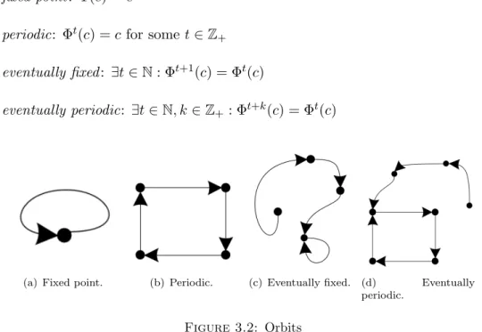
We name the sequence c, Φ(c), Φ2(c), ... the orbit of c. In Figure 3.2 we can observe all possible types of periodic evolutions of any CA:
• fixed point : Φ(c) = c
• periodic: Φt(c) = c for some t ∈ Z+ • eventually fixed : ∃t ∈ N : Φt+1(c) = Φt(c)
• eventually periodic: ∃t ∈ N, k ∈ Z+ : Φt+k(c) = Φt(c)
(a) Fixed point. (b) Periodic. (c) Eventually fixed. (d) Eventually periodic.
Figure 3.2: Orbits
Besides periodic evolutions, cellular automata can still present a non-periodic or a in-compressible non-periodic evolution.
It is common to use graphs, called space-time diagrams, for the representation of the temporal configuration evolution of one-dimensional CA. In these diagrams, configura-tions are depicted horizontally and their evolution are drawn downwards as we can see in figure 3.3. Naturally, these diagrams are only possible for d 6 2.
3.2.5 Neighborhoods
The most usual neighborhood for one-dimensional CA is referred to as the first neighbors neighborhood, and it consists simply of the central cell of the neighborhood and its right and left neighbors: {−1, 0, 1}. Extending this notation for a radius r, the neighborhood set is given by {−r, −r + 1, ..., 0, ..., r − 1, r}, as mentioned in section 3.2.3.
Figure 3.3: Example of a space-time diagram.
For two-dimensional CA, the von Neumann and Moore neighborhoods are the two most common neighborhood shapes (see figure 3.4).
(a) von Neumann neighbor-hood.
(b) Moore neighborhood.
Figure 3.4: The two most common neighborhoods for two-dimensional CA with radius 2.
For d > 1 and radius r these neighborhoods are defined by: Nv(y) = {x | x ∈ Zd, d1(x, y) 6 r}
for the von Neumann, containing (2r + 1)d elements and
NM(y) = {x | x ∈ Zd, d∞(x, y) 6 r}
for Moore’s neighborhood, where d1 and d∞ are metrics associated with the Manhattan norm k y k1 and the maximum norm k y k∞ respectively. For a n dimensional vector y, these norms are given by k y k1=Pni=1|yi| and k y k∞= max{|yi| |i ∈ {1, 2, ..., n}}. Note that in one dimensional CA, the von Neumann and Moore neighborhoods are identical.
Another usual neighborhood is the second-order neighborhood or the neighborhood of the neighborhood, which will be used and explained later, in chapter 5 pp. 70.
3.2.6 Boundaries of Finite Latices
Naturally infinite CA have no boundaries descriptions associated with them. When we are dealing with CA with a finite lattice, the neighborhood used by the local transition function trespass the lattice boundaries. There are two main solutions for this problem: we can either connect the boundaries cells (creating a M¨obius strip for one-dimensional CA or torus for two-dimensional CA), or we can define boundaries values for the values of the trespassed parts of the neighborhood. We name the boundaries of the first solution as periodic or cyclic boundaries. As for the second, there are many possible ways we can set the boundary values, been the two most common the fixed (a constant value on the boundary) and the reflective (reflection of the lattice at the boundary) boundaries. In figure 3.5 we can observe examples, where the 8 central cells represent the finite lattice and the four adjacent cells represent the trespassed parts of the neighborhood.
(a) Periodic or cyclic.
(b) Fixed.
(c) Reflective.
Figure 3.5: Three different types of boundaries.
3.2.7 Classification Systems
Wolfram proposed a classification scheme which divided cellular automata rules into four classes, according to the result of the evolution of the system from an initial state [Wol84]. These Wolfram classes are the following:
• W1: automata of this class die completely after just a few or no steps of evolution. The system evolution leads to uniform fixed point configurations after a finite
number of steps, after which no changes happen. Approximately 86% of the 256 ECA belong to this class. Examples of such rules are 119 and 222.
• W2: evolution leads to a periodically repeating configuration, i.e., after some iterations, configurations starts to repeat themselves. Approximately 9% of the 256 ECA belong to this class. Rules 4 and 126 as examples for this cases.
• W3: evolution lead to a chaotic behavior. Practically all initial conditions leads to patterns that never repeat. Small changes usually spread at a uniform rate and eventually affecting all parts of the system. Approximately 4% of the 256 ECA belong to this class. Rules 30 and 90 are examples.
• W4: evolution leads to localized and propagated structures with complex patterns that can last for arbitrary lengths of time. Only 4 of the 256 elementary cellular automata belong to this class. Examples include rules 54 and 110.
(a) W1 (rule 222). (b) W2 (rule 126).
(c) W3 (rule 30). (d) W4 (rule 110).
However this classification is not unique. Other authors such as Li-Packard [LPL90, LP90], Kurka [K˚97, K˚03] and Culik & Yu [IY88], have also provided alternative classi-fication schemes.
3.3
Reversibility
Reversible cellular automata (RCA) or invertible cellular automata (ICA), are cellular automata capable of recovering the initial state of the automata. In figure 3.7 we can observe two simple examples of reversible rules.
(a) Rule 170. (b) Rule 204.
Figure 3.7: Examples of reversible cellular automata.
Reversible cellular automata are CAs for which the global map is invertible. To be reversible, its global function Φ must be a bijective function Φ : ΣZd → ΣZd. We can say that a cellular automaton A is reversible if there exists a cellular automaton B that reverts it, that is such that:
Ψ ◦ Φ = Identity f unction
where Ψ and Φ are the global functions of A and B respectively. We can then state the following proposition:
Proposition 3.3. [Hed69, Ric72] A cellular automaton is reversible if and only if it is injective.
The problem of deciding if a one-dimensional automaton is invertible, is a decidable problem, even for infinite, one-dimensional CA, as demonstrated by Amoroso and Patt [AP72].
Proposition 3.4. [AP72] It is decidable given a one-dimensional cellular automaton to decide whether it is reversible.
However the reversibility and surjectivity in dimensions higher than one are undecidable. Proposition 3.5. [Kar90, Kar94] It is undecidable given a two-dimensional cellular automaton to decide whether it is reversible.
Because invertible cellular automata constitutes a very small subset of CA [Sea71] and because reversibility can be an undecidable question, we can provide convenient ways to construct reversible cellular automata, providing that we narrow even more the invertible CA set, by ensuring that during the construction of an automaton the backward rule is constructed at the same time as the forward rule. Following we present two simple techniques that can be used to create simple RCA. For other techniques, we refer to the work of Toffoli and Margolus [TM90].
Trivial constructions. They can be build with neighborhood consisting of only one cell [AP72] and with invertible local functions, for instance, permutations of S:
φ : S → S
The simplest case is created by using a local update rule that only copies one of its neighbors. If it copies from the left or from right, we have a simple shift, which is a trivial invertible operation.
Second-order CA. Following the work of Fredkin, Vichniac and others authors [Vic84, Wol02] suggested the use of special rules to achieve invertibility. In these RCAs, the new state of a cell is determined not only by the cell itself and its neighbors one instant back but, also by the cell’s state two instants back (see Figures 3.8 and 3.9). However the reversible rules are not the reverse of the original ones. In figure 3.10 we can see in more detail the differences between a normal rule and a modified one.
Figure 3.8: Simple CA explicitly set to be reversible
Figure 3.9: Simple CA explicitly designed to be reversible.
The configuration ct+1 is determined by the linear combination of the two previous configurations ctand ct−1:
(a) Rule 30
(b) Rule 30R
Figure 3.10: Rule 30 and reversible rule 30R
where c ∈ ΣZd and τ is the dynamic law of the system, which in our case is the global function Φ . By simply rearranging the above formula, we obtain the reverse:
ct−1= τ (ct) − ct+1
In 1977, Toffoli [Tof77] demonstrated that a two-dimensional cellular automaton is Tur-ing complete. However, he left the TurTur-ing completeness of one-dimensional CA as an open problem. This problem was tacked and solved in 89 by Morita and Harao [MH89]. They proved that one-dimensional RCA are Turing complete, by embedding a reversing Turing machine in a one-dimensional RCA, which is in fact a variant type of CA, called one-dimensional partitioned cellular automata. With this variant, they were able to de-sign a globally reversible partitioned cellular automata, capable of simulating a reversible Turing machine. Since a reversible partitioned cellular automata can be simulated by a reversible one-dimensional CA, the Turing completeness was proved.
Brief Overview of Research on
CA-based Cryptography
Ever since the introduction of cellular automata in the cryptographic field, and also because cellular automata have the same expressiveness than Turing machines, cellular automata have found their way into a plethora of encryption schemes, either as their main basis or simply as one of their components. We believe that the presentation of an overview of the most relevant CA-based cryptographic systems and primitives would be useful, both in the contextualization and in laying down the extension of the applicability and usefulness of cellular automata in the development of cryptographic systems.
4.1
Pseudo Random Number Generators
The generation of random numbers is a crucial task in cryptography. They are used not only in the generation of cryptographic keys but also in other crucial parts of crypto-graphic algorithms and protocols, for examples, the generation of initialization vectors. A pseudo-random number generator (PRNG) is a deterministic algorithm that produces numbers whose distribution is indistinguishable from uniform. This cryptographic mech-anism uses an initial seed of randomness (e.g. from some input streams, such as the timing of keystrokes and timing of disk I/O response times [JSHJ98]), and attempts to generate outputs that in practice should be indistinguishable from truly random sources
[SV86, Gut98]. A good cryptographic PRNG should produce a sequence of repeat-able, but high-quality, random numbers. For an excellent overview on PRGs see Knuth [Knu97] and Andreas R¨ock Master thesis [Roc05].
Be as it may be, despite the numerous advices given by various researchers, these are often ignored, resulting in insecure generators, which in turn produces encryption keys that are relatively easier to guess, crippling the underlying cryptosystems where they are used in. Weakly designed PRNGs can easily destroy the security of any system even if strong cryptographic primitives are used.
Presently, linear-feedback shift registers (LFSR) and linear congruential generators are the most popular technique in the design of PRG, because of their compact and simple design. Nonetheless, the LFSR generator is not sufficiently good for cryptographic applications. [Roc05].
The application of cellular automata in cryptographic PRNGs started in the 80’s with Wolfram. In 1985 he suggested a cryptosystem [Wol85] using a PRNG based on one-dimensional CA with periodic boundaries and using rule 30 [Wol86]. The generated random stream is used as the key stream with which the plaintext could be XORed. The random number is obtained from the center cell of the lattice. A stream of random numbers is then obtained from the continuous evolution of the CA. The choice of the center cell as the source of the random bits was based on the fact that this cell pre-sented no significant statistical regularities. During his research, Wolfram noted that the periodicity of the configurations of the automata (the minimum number of evolu-tions required for the automata to repeat a configuration) depends not only on the size of the cellular space but also on the initial seed. His PRNGs was able to pass a suite of seven statistical tests, even surpassing classical PRNGs based on LFSR of the same size, but not as good as linear congruential generators. According to his estimations, if the cellular space of the automata is larger than 53 cells, its maximum period should be approximately 20.61N, where N represents the size of the cellular space. Wolfram noted that the statistical properties of the random stream is better if its size is much shorter than the period of the generator.
In 1991, Meier et at. [MS91] broke Wolfram’s cryptosystem with chosen plaintext at-tacks where they demonstrated that the sequence of configurations of the system is not hard to recover. Wolfram [Wol86] also claimed that the problem of recovering the seed of
its PRNG was an NP-complete problem. However, Koc and Apohan [KA97] proved that this was not the case and they presented a computationally feasible algorithm capable of inverting rule 30 in O(n) for some seeds and O(2n/2) in the worst case.
To increase the period and the statistical properties of CA-based PRNGs, a new type of CA emerged: the hybrid or non-uniform CA, where instead of a single rule, the automata uses multiple rules. To practically achieve this flexibility, a new type of CA structure emerged: the programmable CA (PCA) [NKC94]. In figure 4.1 we can observe a simplis-tic representation of the structure of a PCA, with which we can form different additive CAs (one having a combination of XOR and XNOR rules), by simply manipulating the controlling signals, which controls which neighboring cells are combined. This flexible
Figure 4.1: Structure of an additive PCA.
structure enables the use of nonlinear enciphering functions, capable of generating a large number of multiple keys.
Hortensius et al. [HMC89, HMP+89] proposed a non-uniform cellular automata, consist-ing of a pair of rules, (90, 150) or (30, 45), with the intent of generatconsist-ing test vectors in VLSI manufacturing. Statistical tests showed that the performance of these generators exceeded Wolfram’s. They also noted that non-uniform CA with null boundary had on average longer period. Hortensius at al. also demonstrated that their CA had a better statistical performance than LFSRs.
Nandi, Chaudhuri and Kar [NKC94] proposed a block and stream cipher but, they focus their attention on non-uniform CA with null boundaries, operating exclusively with linear rules (rules that exclusively employs XOR logic operations), namely rules
51, 153 and 195 for block ciphers and rules 90 and 150 for stream ciphers. However their block scheme was broken by Murphy et al. [BBM97]. Another successful attack on Nandi et al. cryptosystem was made by Mihaljevic [Mih], but this time using only ciphtertext. In the attempt of eliminating the weakness present in [NKC94], Sen et al. [SSC+02] combined affine and affine transformations in order to achieve non-linearity. However, Bao [Bao03] was able to show that the cryptosystem based on this combination could also be easily broken with a chosen-plaintext attack and with low computational cost.
Rubio et al. [REW+04] tested 28 linear hybrid CAs, formed by the combination of two linear ECA, for example (60, 90), where the corresponding rule to apply to any cell is dependent on its current state. For their tests, they considered both periodic boundaries and null boundaries and also several random initial configurations. They tested their pseudorandom properties through a battery of cryptographic statistical tests, such as frequency, serial and poker tests. Because Meier & Stafelbach [MS91] demonstrated the feasibility of attacking PRGs generators with a size lesser than 500 cells, with attacks based on the algebraic properties of CAs, Rubio et al. considered hybrid CAs with 512 cells. From the 28 rules only 10 hybrid CAs with periodic boundaries and 3 with null boundaries passed the tests.
More information on non-uniform CAs with null boundaries and its relation with length cycle and their application on encryption schemes can be consulted in the works of Anghelescu et al. [Ang11, AIS07, AIB09].
From the results of the studies mentioned above, we see that for a PRNG to provide both a good randomness quality and a satisfactory period length, the choice of the transition rules is of the utmost importance. Because of the sheer number of rules and CA configurations, many researchers turned into methods of automatically select the best set of rules for a given CA. Among those methods we find the use of genetic algorithms. Tomassini et al. [ST96] demonstrated that the use of genetic algorithms can give birth to good PRNGs. These algorithms usually employ entropy as the fitness function to trigger mutations. However, high entropy is a necessary but not sufficient condition for a good quality PRNG, and therefore statistical tests should also be applied after the evolution and selection of the PRNG. Tomassini showed that a good PRNG can be obtained by randomly mixing the rules 90, 105, 150 and 165. Tomassini and
other researchers continued their work on evolutionary rules selection, giving rise to a plenitude of papers [TP01, GZ03, TSZP99, SBZ04, SSB06, TSP00].
4.2
Block Encryption With Second-Order Cellular Automata
In a second-oder CA, the state of each cell at instant t + 1 depends on the neighborhood state configuration at t and the state of the cell at t − 1:
φt+1(x) = f (φt(x − r), ..., φt(x), ..., φt(x + r), φt−1(x − r), ..., φt−1(x), ..., φt−1(x + r))
where φt(x) is the state of cell x at instant t, f the local transition function and r the neighborhood radius.
With this extra dependency and associating two elementary cellular automata we are able to build reversible rules. The two ECA rules R1 and R2, must be related to each other by the condition:
R2 = 2d− R1− 1
where d = 22r+1. The first rule defines the state transition when the cell at instant t − 1 was in state ‘1’, and the second one when the cell was in the state ‘0’. For example, selecting R1 = 30 and r = 1 we have R2 = 22
3
− 30 − 1 = 225, then we can represent our second order rule by:
Next we present how these second order reversible rules can be used in a cryptosystem. After the set of the first two configurations (for example, with random data and plain-text), the encryption process is done by evolving the CA by a pre-defined number of k steps, as illustrated in figure 4.2. When encryption is complete, the last configuration is considered residual or junk data, which can be XORed with the private key. The
last but one configuration is our ciphertext. Since every step requires the two previous configurations, these two final configurations (the residual and the ciphertext) should be saved, since they are going to be required for the decryption process as the two initial configurations of the automata. The CA then must iterate the same number of steps as in the encryption process, k steps, and the resulting next to last configuration is then the recovered plaintext.
(a) Encryption. (b) Decryption.
Figure 4.2: Simplified encryption and decryption process.
Since is quite obvious that a cryptosystem based merely on a single second order re-versible rule and on a few iterations is not safe, Bouvry et al. [SB04b, SB04a] suggested a more secure cryptosystem. In their system, the two initial configurations of the CA are populated by random data and by the plaintext as illustrated. To increase security, they used multiple rounds of data manipulation and transformations. One round of this system can be seen in figure 4.3 (source: [SB04a]). The system is composed by four one-dimensional CA: CAL, CAR, CAC and CAS. All CA are radius-2 except for CAC which is radius-3. Each plaintext block is 64 bits long and the key is 224 bits, which specifies the four RCA rules to be used and number of evolutionary steps. CAL, CAR and CAS are composed of 32 cells and CAC by 64 cells. Encryption of each plaintext block is composed of a predefined number of rounds, where the data suffers splittings, shiftings, recombinations and configuration evolution in each round by the respective
Figure 4.3: Single round of Bouvry’ system.
CA: CAL and CAR applies the MCA rule to the left and right part of the data respec-tively k1 times, CAC applies the MCA rule to all bits of the data k2 times and CAS generates the shift to apply. The initial data is randomly generated and if CBC mode is used, the final data will be used as the initial data for the subsequent encryption blocks. In addition of saving the generated ciphertext, the final data and the final two configurations of CAS must also be saved. The decryption process is done by reversing the order, including the shifts. The number of evolutionary steps required by each CA to achieve an avalanche effect and optimal effect were obtained through experimental evaluation.
Brute force attacks on the key is out of question, as a result of the key space size: 2224. It is also computably infeasible to discover the initial configurations of the automaton.
Although finding the configurations of CAC and CAS (264 and 232respectively) is com-putationally feasible, the attacker would still have to test all 232possible configurations of both CAL and CAR, if he uses a brute force approach. To prevent any possibility of brute force attacks, the block size can be increased, for instance, from 64 to 128 bits.
4.3
Secret Sharing Schemes
Usually, in secret sharing schemes, a secret is shared between different parties so that only a selected subset of those parties can recover the secret. Applications of such schemes in-cludes the Byzantine agreement [Rab, Wan11], multi-party computations [CDM], access control [NW98], threshold cryptography [DF92], attribute-based encryption [GPSW] and e-voting [Sch99].
In a (k, n) threshold scheme, the secret S, is decomposed by a trusted authority, called a dealer, into n pieces and each piece is distributed among n parties in such a way that the only way to reconstruct the secret is if k or more parties get together their pieces. The quantity of information of each party in this scheme is uniform, i.e., the secret is equally shared among members in a group and where every member has an equal amount of partial information. A series of (k, n) threshold schemes were simultaneously introduced during the 70’s by Shamir [Sha79] and Blakley [Bla79].
Since all existing works tackle this problem in a similar way, we first define a few common concepts. As we have seen in the previous section 4.1, pp. 31, a linear cellular automata (LCA) is a CA with rules that exclusively employs XOR logic operations, i.e., the next-state is determinate by a function that employs only XOR logic operations. Hence, the state of each cell is updated according to equation (3.1), which now assumes the following form for one-dimensional LCA with a neighborhood N radius-r:
φt+1(i) = r X
j=−r
αjφt(i + j) (mod 2), ∀i ∈ Z, 0 6 i 6 |N| − 1,
where φt(i) denotes the state of cell i at instant t and ∀j : αj ∈ Z2. Because there are 2r + 1 neighboring cell (including the origin) for each i, there are 22r+1 LCAs and each
one can be specified by an integer w called rule number, which is defined by: w = r X j=−r αj2r+j, 0 6 w 6 22r+1− 1
However, as we have seen in section 3.3, we can also make the state of a cell at t + 1 depend not only on its state and of its neighbors at t, but also on the state of those same cells or of some other groups of cells at t − 1, t − 2, ..., t − k. This CA is then called k-th order cellular automata or memory cellular automata (MCA). A k-th order linear memory cellular automata (LMCA) the state transition of each cell is given by:
φt+1(i) = f1(Vit) + f2(Vit−1) + · · · + fk(Vit−k+1) (mod 2), ∀i ∈ Z, 0 6 i 6 |N| − 1, (4.1) where fi represents the local transition function of a particular LCA with radius r for 1 6 i 6 k and Vit ⊂ (Z2)2r+1 denotes the states of the neighbors of cell i. Because of its dependency on previous configurations, to start its evolution, the k-th order LMCA, requires then k initial configurations (Φ0(c), · · · , Φk−1(c)), where Φ0(c) = c represents the initial configuration of the CA.
The application of automata in secret sharing schemes, was introduced in 2003 by Enci-nas et al. [MEdR03]. They proposed a (k, n)-threshold scheme based on two-dimensional LMCA with periodic boundaries, Moore neighborhood with radius 1 and an alphabet S. They targeted specifically images of size r × s bits as the secret, and therefore the number of cells of the CA is r × s. Since we are dealing now with two-dimensional CA, the above equations should be modified in order to consider two-dimensional cellular automata with Moore neighborhood. The state of cell (i, j) is now updated according to:
φt+1(i, j) = X β,γ∈{−1,0,1}
αβ,γφt(i + β, j + γ) (mod c),
with 0 6 i 6 r − 1, 0 6 j 6 s − 1, αβ,γ ∈ Z2 and c = 2b denotes the number of colors of the image (b&w image, then b = 1; for gray-level images; b = 8, if color image, b = 24). Because each cell has now 9 neighboring cells, there are 29 = 512 possible two-dimensional LCAs and each one is specified by the rule number w, which is given
by:
w = α−1,−128+ α−1,027+ α−1,126+ α0,−125+ α0,024+ α0,123+ α1,−122+ α1,021+ α1,120,
with 0 6 w 6 511.
Let Vijt ⊂ (Z2)9 denote the state of the neighboring cells of cell i. Equation (4.1) now becomes: φt+1(i, j) = k−1 X m=0 fm+1(Vijt−m) (mod c) (4.2) with 0 6 i 6 r − 1, 0 6 i 6 s − 1 and as before fl, with 1 6 j 6 k, denotes the local update function of some k two-dimensional LCAs. Equation (4.2) is reversible if the following condition holds:
fk(Vijt−k+1) = φt−k+1(i, j)
Then the inverse is another another LMCA with local transition function given by:
φt+1(i, j) = − k−2 X m=0 fk−m−1(Vijt−m) + φt−k+1(i, j) (mod c) (4.3) with 0 6 i 6 r − 1, 0 6 i 6 s − 1.
In this scheme, both the shared and the recovered image have the same size as the original. Also, Φ0(c), Φ1(c), ..., Φk−1(c) are populated both with data from the image and with random matrices. The configuration Φ0(c) is populated with the secret image, while the others k − 1 configurations are randomly generated. Each participant or group receives one subsequent CA configuration randomly selected, i.e., if there are n participants, then each participant will receive one of the n final configurations of the CA. Summarizing the main steps of the system:
1. Setup phase:
• The dealer generates a sequence of k − 1 random integers where each number corresponds to a respective update function, {w1, · · · , wk−1}, where 0 6 wl6 511 and 1 6 l 6 k − 1.
• The dealer constructs equation (4.3) with fwl : (Zc)
• The dealer populates the configurations {Φ0(c), Φ1(c), ..., Φk−1(c)}, where the configuration Φ0(c) stays with the bit representation of the secret image while the remaining k − 1 configurations are randomly populated.
2. Sharing phase:
• The dealer evolve the two-dimensional CA m + n − 1 steps, by choosing m and ensuring that m > k (to avoid overlaps between initial configurations and shares);
• The dealer then distributes to each of the n participant, one of the last n consecutive final configurations of the CA, {Φm(c), Φm+1(c), ..., Φm+n−1(c)} and the set rules generated in the previous phase, so that the reverse of the linear equation (4.3) can be constructed.
3. Recovery phase:
• Obtain a set of consecutive k shares of the form {Φm+α(c), Φm+1+α(c), ..., Φn+m−1+α(c)} with 0 > α > n − k;
• By inverting the configuration order and iterating m + n − 1 times the inverse of equation (4.3), we are able to recover the initial configurations of CA including the secret image (Φ0(c)).
According to the authors, the security of the system lies on the fact that if any of the k configurations is missing, we would need to solve an underdetermined system in order to recover the secret image.
In 2008, Encinas et al. [AEdR08] extended their previous work [MEdR03] to a (n, n)-threshold multi-secret sharing secret scheme, such that that each of the n participants shares a secret color image out of n. Unlike in their previous work, where the initial con-figurations were populated with both the secret image and random data, in this scheme, all secret images populate the n initial configurations of the CA. During the setup phase, each image can be padded, if necessary, in order for all images to have the same size. As before, the final size of the automata depends on the number of bits of the images. The security of this system was demonstrated to be utterly capable of resisting the most important statistical attacks. As before, the absence of a single part of the secret leads to a underdetermined system of linear equations. The scheme presented excellent values
for both the confusion and diffusion properties and also presented good statistical results.
Despite the good security results of the above schemes, Jafarpour et al. [JNKS07] proved that they are vulnerable against dishonest participants collusion by either cheating with bogus shares or with bogus transition rules. These cheats allows L cheaters, with L ≤ k, to obtain the correct secret by computing the cheating value for every cell at each step, while the others participants receive corrupted shares without knowing that cheating is done in the background. To reduce this vulnerability, authentication methods were introduced, such as the ones by Eslami et al. [EA10, ERA10] and Sujata et al. [SS13].
4.4
S-Boxes
Substitution Boxes or S-Boxes are fundamental pieces in symmetric cryptosystems, such as, DES [NBoS77], Blowfish [Sch94] and AES [PT01]. In general, an S-Box takes m input bits and transforms them into n output bits. Basically there are n component functions each being a map from m bits to 1 bit, i.e., each component function is a Boolean function in m Boolean variables. This is called an m × n S-Box and is often implemented as a lookup table. These S-Boxes are carefully chosen to resist linear and differential cryptanalysis.
Since cellular automata have the same expressiveness as Turing Machines, any Boolean function can be simulated with a cellular automata. Also, considering that S-Boxes are merely Boolean functions that map n inputs to m outputs, we are able to create CA-based S-Boxes, where the automata generates a n bit output through the temporal evolution of a n bit input (the seed of the automata). Szaban and Seredynski [SS08] provide an excellent example of how such system can be implemented with cellular automata. Their system corresponds to a 8 × 8 S-Boxes similar to the AES S-Boxes. The configuration vector of the system contains all the necessary information: the initial state of the CA, rules, number of evolutions and which cells work as the input (the output cells are the same a the input). The applied rules were selected after a series of tests, where non-linearity and autocorrelation were measured at different evolutionary instants. The injectivity of the box were also measured for different CA sizes. These measurements are essential to increase the security of the system against differential