WORKING PAPER SERIES
Universidade dos Açores
CEEAplA WP No. 02/2011
Evaluation of the Surrender and the Minimum
Guaranteed Rate of Return Options in Life
Insurance Products
Pedro Pimentel Ricardo Pereira
Evaluation of the Surrender and the Minimum
Guaranteed Rate of Return Options in Life Insurance
Products
Pedro Pimentel
Universidade dos Açores (DEG e CEEAplA)
Ricardo Pereira
University of Cambridge (Department of Land Economy)
Working Paper n.º 02/2011
Janeiro de 2011
RESUMO/ABSTRACT
Evaluation of the Surrender and the Minimum Guaranteed Rate of Return Options in Life Insurance Products
This paper aims to value a Guaranteed Investment Contract (GIC), offered by insurance companies, with a minimum rate of return and an option to surrender the contract (surrender option) at any time before the maturity date. The valuation framework uses a set of different models to value each one of these two options included on a GIC contract commercialized by a Portuguese financial group. We estimate that the surrender option value is around 1.18 percent of the net premium and that the value for the minimum guaranteed rate of return option varies between 0 an 7 percent, according to the used model.
JEL: G13, G22, G24
Keywords: Guaranteed investment contracts, insurance, options
Pedro Pimentel
Universidade dos Açores
Departamento de Economia e Gestão Rua da Mãe de Deus, 58
9501-801 Ponta Delgada Ricardo Pereira
University of Cambridge Department of Land Economy 19 Silver Street
Rate of Return Options in Life Insurance Products
Pedro Miguel Pimentel
Finance Assistant Professor
University of the Azores
Business and Economics Department
CEEAplA
ppimentel@uac.pt
Ricardo Pereira
University of Cambridge Department of Land Economy
19 Silver Street Cambridge, CB3 9EP UK
ramgp2@cam.ac.uk This draft: December 2010
Abstract
This paper aims to value a Guaranteed Investment Contract (GIC), offered by insurance companies, with a minimum rate of return and an option to surrender the contract (surrender option) at any time before the maturity date. The valuation framework uses a set of different models to value each one of these two options included on a GIC contract commercialized by a Portuguese financial group. We estimate that the surrender option value is around 1.18 percent of the net premium and that the value for the minimum guaranteed rate of return option varies between 0 an 7 percent, according to the used model.
JEL: G13, G22, G24
1. Introduction
One of the most important challenges facing many advanced economies today is the increasing proportion of the elderly in the population, and thus the requirement for increased provision of pensions and medical care. Given that income from pension funds may not be sufficient to cover retirement needs, many of this age group will have to seek income from other assets. As a consequence, during the last few years, insurance companies developed a set of new products more forward looking to single investors necessities. Therefore, we observed the development of financial contracts/products that besides their attractive financial features (such as, minimum guaranteed rates of return) they also have taxes benefits.
This paper aims to value a Guaranteed Investment Contract (GIC), one of those products developed and offered by the insurance companies. We focus in a GIC, commercialized by a Portuguese financial group, that provides a minimum rate of return and the possibility to benefit from capital returns linked to the performance of a reference fund. This product does not provide insurance against mortality risk and confers the option to surrender the contract (surrender option) at any time before the maturity date.
The minimum guaranteed rate of return constitutes a floor for the contract returns. In terms of evaluation, detaining a contract which confers this right is equivalent to possessing a call option on a zero coupon bond (ZCB) which has an effective return equal to the minimum rate. The assessment of this call option value is a key element for the insurance company, since it is exposed to the performance of the reference fund.
The evaluation of the two options mentioned previously is the main purpose of this paper. The layout of the rest of this paper is as follows: Section 2 presents an overview of the surrender option and of the minimum guaranteed rate of return option pricing models. Section 3 reports the results of the valuation models. Section 4 presents some conclusions remarks and outlines paths for future investigations.
2. Literature Review 2.1. Surrender Option
Several life insurance products offers to their holders a set of different options, such as, the anticipated surrender option, the option to profit from a minimum rate of return, the option to renew the contract, amongst others, which makes the valuation of these products very complex..
According to Hunziker and Koch-Medina (1996) the majority of the life insurance contracts that comprise a single premium can be seen as a structured product with:
- zero coupon bond features; - options’ features; and
- vanilla insurance products features.
Hence, standard actuarial models, traditionally used by insurance companies, are not longer reliable and able to value these products. The actuarial models simply ignore and expurgate from the value of these products the value of underlying options.
Economic intuition tell us that an investor will exercise the surrender option if there is a financial product with similar characteristics which enables him a net rate return above the one of the existent product. However, there are non-rational reasons for the exercise of the surrender option, such as a shortage of liquidity. This last situation constitutes a contingency which turns the evaluation of this right more complex. Smith (1982) by realizing that many insured people did not surrender their contracts in favour of investments with superior rates of return, has denominated this phenomenon as a puzzle. The author argues that the tax benefits only explain a part of the puzzle.
Smith (1982) demonstrates that a life insurance contract represents a unique investment opportunity and should be evaluated as such, since it offers a set of options, which replication is unavailable. According to the author, the value of these options, which is an important part of the contract value, influences the effective rate of return of these life insurance products.
Albizzatti and Geman (1994) develop a closed form solution to value the surrender option assuming that interest rates follows a stochastic process. The authors consider the surrender option as a put option written by the insurance company at time t with maturity T, that equals the maturity of the insurance contract.
( )
tR( )T( )
( ) ( )
t t t d N d N t B e C 0 = λ 0, 0, 1 − 2( ) (
)
( )
( )
t T VarR T t VarR T T t f t dt , , 2 , , 0 1 + + − = γ(
)
(
(
) ( )
)
( )
t T VarR T t R t T t R t T d dt t , , , , cov 1 2 − − − = where-
λ
R ,( )
0T represents the annual effective return of a ZCB with maturity T , free of chargeand commissions, with 0<λ<1;
- B ,
( )
0 t the present value of the expected value at time t of a ZCB with maturity in T ; - N(.) represents the cumulative function of a normal distribution;-
( )
( ) ( ) ( ) ( )
[
K t]
t T T R t T T tβ
λ
γ
− − − −= 0, 1 ln 1 , where K
( )
t is the net income of taxesresulting from the surrender option exercise and
β
represents the commissions of subscribing a new insurance contract;- f
(
0,t,T)
the forward rate observed at moment zero regarding the period[
t,t+T]
; - R ,( )
t T represents the return of a new contract subscribed in t immediately after theexercise of the surrender option of the previous contract, which is the same return of a ZCB with maturity T , which market value in t is B
(
t,T+t)
=e−TR( )t,T .The Albizzati and Geman (1994) model is very similar to the one of Black & Scholes (1973). Considering that the surrender option is nothing less than an exchange option of one asset for the other, this model is also identical to Margrabe (1978) model, but generalized towards a context in which the interest rates follow a stochastic process.
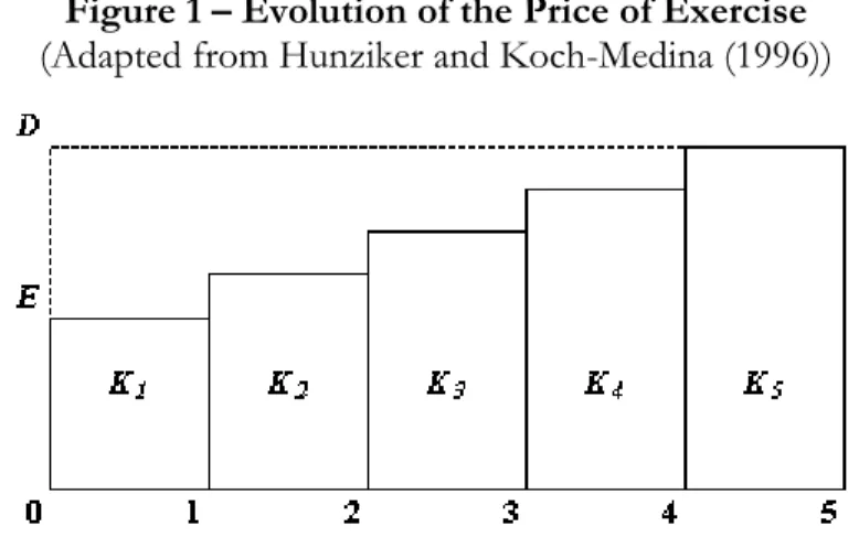
Hunziker and Koch-Medina (1996) develop a model to value a single premium insurance contract, E, that pays a minimum rate of return i% per year, plus rt%, which is function of the
performance of the reference fund, compound until the maturity date T. In maturity, the insured capital, D, would correspond to the nominal value of a ZCB. Analytically, we haveD=E*
∏
Tt=1(
1+i+rt)
. In this perspective and considering the existence of the surrenderoption, Hunziker and Koch-Medina (1996) argue that this position can be replicated by a long position on a put and a short position on a call, both american, on a ZCB with redemption value of D and with exercise prices equal to the compound value of the premium until the moment of the exercise, Kt1 (Figure 1).
Figure 1 – Evolution of the Price of Exercise
(Adapted from Hunziker and Koch-Medina (1996))
The insurance company is long on a call option that pays Rt =
{
St −Kt}
+ max 0; and short on a put option that paysRt =
{
Kt −St}
− max 0, , both with the same characteristics of the options described above. Note that the exercise price is time dependent and equals the book-value of the ZCB, ZBt, in each moment of time. In this context, insurance company is exposed to the risk
that at any time the exercise price of the put option is different from the market price of the ZCB, St., i.e Kt ≠St.
1 Neglecting others costs, commissions and penalties incurred from the anticipated surrender, which in case of
having been taken in consideration would reduce the exercise value. Alternatively the values charged in the contract surrender may be seen as the price of the option.
As the surrender option not always is exercised rationally, grouping a big number of independent contracts enables an effective cover, regarding the risk of all the insured people to exercise the option rationally, forcing the insurance company to incur in losses and financial distress.
Considerpt,ras the surrender probability in the whole of the insurance contracts. This
probability considers surrender by death (t) and by rational and irrational reasons (r). The latter reasons are a key variable in the valuation of this contract and can be estimated based on historical data of the insured person behaviour or based on stylized data related to the anticipated mortgages payments.
The value of the surrender option is based on the expected losses,Rt−, that occurs from the
rational exercise of the option and from the expected gains, Rt+, that occurs from the non
rational exercise of the option, as well as the expected gains and losses occurring from the death of the insured person. The authors defend that this methodology is option pricing theory consistent but, implies the specification of a stochastic process for the interest rates since ZCB prices are very sensible to this variable.
Reisman (2000) adapts a bond valuation model with default risk and stochastic interest rates to the valuation of the surrender option of the life insurance contracts, considering that the default is analogous to the death of the insured person. The model is derived based upon two alternative assumptions, the optimal surrender and the noisy or non-optimal surrender. The optimal surrender implies that the investor is rational and only exercises this option if he is capable of maximization his wealth, while the noisy surrender is modelled through the specification of an exogenous process
Grosen and Jorgensen (1997) conclude that the difference between the values of the American and European options on the minimum rate of return of the contract is the value of the surrender option. The authors also demonstrate that for longer maturities, the difference between the value of the two types of options (the value of the surrender option) increases.
2.2. Minimum Guaranteed Rate of Return Option
The evaluation of the minimum guaranteed rate of return option implies a review of the traditional evaluation models of the interest rate derivates and a review of the stochastic processes which characterize the evolution of the interest rates.
2.2.1. Traditional Evaluation Models of the Interest Rate Derivates
Hull (2000, p. 530) refers that the interest rate derivates are more complex to evaluate then the other derivates because:
- The interest rates do not follow the traditional geometric brownian motion (GBM);
- to value many products, we need a model that describes the entire yield curve (in which the volatility is not constant);
- The interest rates define derivative’s payoffs and are used for discounting them.
Considering that the financial product under investigation has features of an interest rate floor, in this section, we describe how the standard model (Black’s model) can be used to value it.
An interest rate floor provides a payoff when the interest rate on the underlying asset falls below a certain rate. So, a floor provides a payoff at time tk+1 (k = 1, 2, …, n) of
Lδk max.(RX – Rk, 0) (1)
where δk = tk+1 - tk, L is the notional or main value, RX is the minimum rate of return and Rk is the rate of return of the alternative product, between tk and tk+1. A floor may be analyzed as a call options portfolio of an interest rate or a ZCB put options portfolio. Each one of these options is named of floorlet, which payoff is defined by the equation (1). If the Rk rate follows a lognormal distribution, with σk volatility, the floorlet value is given by the equation
Lδk P(0, tk+1)[RXN(-d2) – FkN(-d1)] (2) where,
P(t, T) – price at moment t of a ZCB which pays € 1 at moment T Fk –Forward interest rate between tk and tk+1
d1 = k k k 2 k X k t σ 2 t σ + R F ) ( ) ln(
d2 = d1 - σk t k
Each floorlet of a floor must be valuated isolatedly using the equation (2) and we may use a different volatility for each floorlet (forward or spot volatility). Alternatively, we may use the same volatility for each floorlet which constitutes the floor (flat volatility). This model assumes that interest rates are constant or deterministic, which allow us to assume that forward price of an asset is equal to its future price. When interest rates are stochastic, this model has limitations because the forward price and the futures price are not the same and the discount rates are not constant.
2.2.2. Interest Rate Derivates: Stochastic Processes
In the model presented in the previous section, we assume that the interest rates follow a lognormal probability distribution. However, this distribution does not describe the interest rate behaviour. In this section, we discuss other models to build a term structure model.
Applying the notation presented previously, the ZCB value, at moment t (designated by P(t, T)), which pays €1 at moment T > t, is
P(t, T) = EP
t [mt(T)]
where mt(T) is the rate of marginal substitution or the pricing kernel and EP[.] is the expectations
operator under the original probability P. Using a martingale equivalence, the price of a ZCB can be expressed as P(t, T) = EQ t [ ∫ e rsds T t -] (3)
where EQ[.] is the expectations operator under the probability neutral to venture Q and r
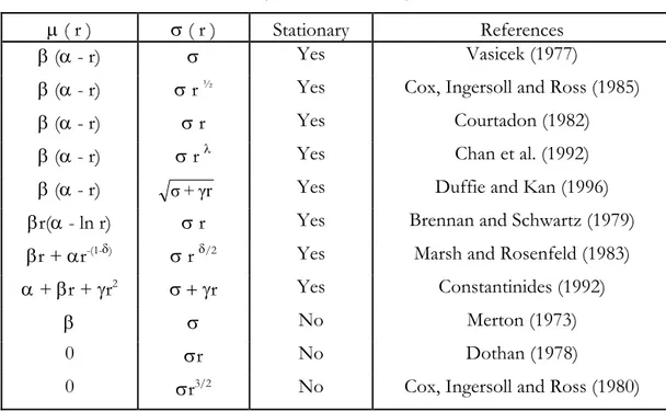
s is the instantaneous rate of return of the asset free of risk. Several articles use the following univariate stochastic process in the development of the ZCB valuation equation
dr = µ(r)dt + σ(r)dWt (4)
Wt is the traditional brownian motion process. Table 1, adapted from Sundaresan (2000),
Table 1 – Alternative Specifications for the Spot Interest Rates Process
(Univariate Models)
µ ( r ) σ ( r ) Stationary References
β (α - r) σ Yes Vasicek (1977)
β (α - r) σ r ½ Yes Cox, Ingersoll and Ross (1985)
β (α - r) σ r Yes Courtadon (1982)
β (α - r) σ r λ Yes Chan et al. (1992)
β (α - r) Yes Duffie and Kan (1996)
βr(α - ln r) σ r Yes Brennan and Schwartz (1979)
βr + αr-(1-δ) σ r δ/2 Yes Marsh and Rosenfeld (1983)
α + βr + γr2 σ + γr Yes Constantinides (1992)
β σ No Merton (1973)
0 σr No Dothan (1978)
0 σr3/2 No Cox, Ingersoll and Ross (1980)
The majority of these models start by arguing several economic variables and only afterwards derivate a process for the short term interest rate, r, so that they are called equilibrium models. In a multivariate model, the process of r involves only an uncertainty source. In the equation (4), the drift, µ, and the volatility, σ, are functions of r and are constant. Hull (2000) does an exposition of the Vasicek and Cox, Ingersoll and Ross models and states that the short term interest rates revert to mean. About the first model, which incorporates the mean reverting process and that it will be used in the next section, the interest rate at the short term revert the level α with a β velocity. The stochastic term, σ dz, follows a normal distribution. Using the equation (3) Vasicek (in Hull, 2000, p. 567) obtains the following expression for the price, at moment t of a ZCB which pays € 1 at moment T:
P(t, T) = A(t, T)e-B(t, T)r(t) (5)
Where r(t) is the value of r at moment t, B(t, T) = β e 1- -β(T -t) A(t, T) = exp [ β 4 T t B σ β 2 σ α β + T t B 2 2 2 ) , ( -) / -t)( T -) , ( ( 2 2 ] R(t, T) is the interest rate constituted at moment t with a maturity T-t,
r γ + σ
R (t, T) = ln ( , ) ( ) t -) , ( ln t -- B t T r t T 1 + T t A T 1 (6) Through this equation, after the gathering of β, α and σ, we may define the temporal structure of the interest rates as a r(t) function. Jamshidian (in Hull, 2000, p. 567) shows that the price, at moment zero, of an European put option, with maturity T, under a ZCB, which pays L, using the Vasicek model is
LP(0, s) N(h) – XP(0, t)N(h - σP)
s is the bond’s maturity, X is the price of the exercise,
h = 2 σ + X T 0 P s 0 P L σ 1 P P ( , ) ) , ( * ln σP=
[
]
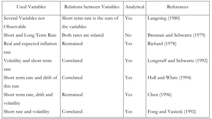
β 2 1 × e 1 × β σ β β(s-T) -2 T - -e-Sundaresan (2000) argues that the univariate models have the advantage of being easy to implement, but do not pick up the diversity verified in the temporal structures of the interest rates. For this reason, multivariate models were developed. Sundaresan (2000) also does an exposition of these models concerning the variables used by the authors (Table 2).
Table 2 –Multivariate Models
Used Variables Relations between Variables Analytical References
Several Variables not Observable
Short and Long Term Rate Real and expected inflation rate
Volatility and short term rate
Short term rate and drift of this rate
Short term rate, drift and volatility
Short rate and volatility
Short term rate is the sum of the variables
Both rates are related Restrained Correlated Correlated Restrained Correlated Yes No Yes Yes Yes Yes Yes Langetieg (1980)
Brennan and Schwartz (1979) Richard (1978)
Longstaff and Schwartz (1992) Hull and White (1994) Chen (1996)
The major disadvantage of the equilibrium models is that they do not adjust automatically to the present temporal structure of the interest rates. Therefore, they are not accurate2 pricing models.
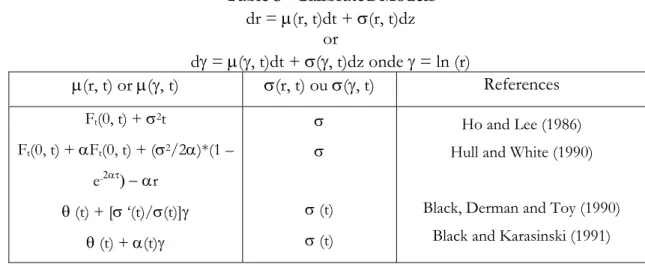
An important development in this area is the models that can be calibrated. These models are no-arbitrage. In a no-arbitrage model the present temporal structure of the interest rates is an input and the drift of the interest rates is variable in time. Sundaresan (2000) does a quick exposition of the models that enable calibration, which is reproduced in Table 3.
Table 3 –Calibrated Models
dr = µ(r, t)dt + σ(r, t)dz or dγ = µ(γ, t)dt + σ(γ, t)dz onde γ = ln (r) µ(r, t) or µ(γ, t) σ(r, t) ou σ(γ, t) References Ft(0, t) + σ2t Ft(0, t) + αFt(0, t) + (σ2/2α)*(1 – e-2ατ) − αr θ (t) + [σ ‘(t)/σ(t)]γ θ (t) + α(t)γ σ σ σ (t) σ (t) Ho and Lee (1986) Hull and White (1990) Black, Derman and Toy (1990)
Black and Karasinski (1991)
In all these models, the dynamics of the interest rates at the short term depend on the initial forward curve, F(0, t), and the drifts and diffusion coefficients vary through time.
3. Options’ Assessment
To appraise the surrender option we apply the methodology developed by Hunziker and Koch-Medina (1996), exposed in section 2. The minimum guaranteed rate of return option is valuated by the following models:
1. Black’s Model (also described in section 2); 2. Binomial Model;
3. Monte Carlo Simulation.
3.1. The Surrender Option Assessment
The surrender option assessment through the Hunziker and Koch-Medina (1996) methodology was accomplished for a life insurance product that guarantees a 4 percent minimum rate of return, issued in 1997 by a Portuguese financial group. Although the product has a maturity of 15 years, we have considered 8 years, so that real data can be used for the majority of the parameters used in the methodology. In 1997 were subscribed about 2.030 contracts of this type of product with a total amount of insurance capital rounding the 32.12 millions of euros.
Table 4 reports the observed surrender probabilities ,pt,r, that include surrenders based on rational and non rational motivations.
Table 4 – Surrender Probability
Source: Financial Group.
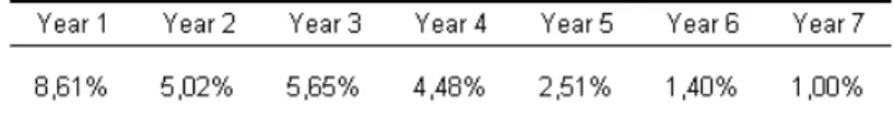
Table 5 exposes the observed rate of return of the product over the all period.
Table 5 – Net Return of the Contract –
i
As alternative rate of return, r, we consider the yield rate of a ZCB that matches the maturity of the insurance product, observed at the beginning of each year (Table 6).
Table 6 – Yield Rate of the ZCB
The rates reported in Table 6 besides being used to appreciate the rationality of the exercise of the surrender option, are also used to mark to market the ZCB value.
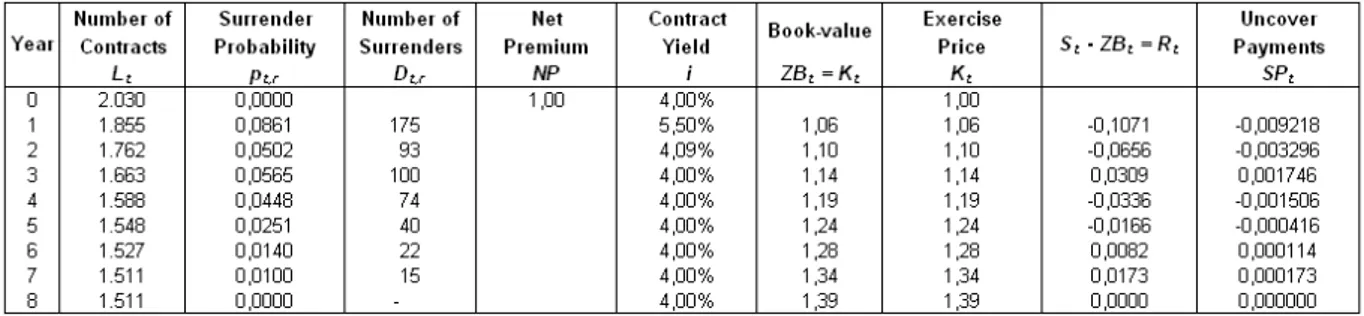
Table 7 reports the expected3 gains and losses incurred by insurance company given the death of
the insured person and the rational and non-rational exercise of the surrender option for a nte premium of 1 m.u..
Table 7 – Expected Gains and Losses Incurred by the Insurance Company under the Exercise of the Surrender Option
Discounting4 the value of the gains and losses incurred by the insurance company from the
exercise of the surrender option, we obtain the surrender option value, which adds up to 1.18 percent of the value of the insurance contract. This value can be paid in the subscribing moment or in the moment of the exercise, through the payment of penalties. In the latter case we have a type of exotic option, given that surrender option value is liquidated at the moment of the exercise. In the product in analysis, there are penalties only for the first five years of the contract., meaning that after this data the surrender option is valueless for the insurance company. Considering the surrender probabilities (Table 4) and the penalties established in the contract for the first 5 years5, the expected present value of penalties is around 0.95 percent for each net
premium m.u., which means that the insurance company is undervaluing the surrender option. As argued by Grosen and Jorgensen (1997) the value of this option for a longer contract should be substantially higher to the computed value.
3SPt = Rt * pt,r , with Rt = Rt++ Rt-
4 The actuary rate used for each period is the yield, at moment zero, of the ZCB with maturity of 1, 2, 3, 4, 5, 6, 7
and 8 years. These rates were provided by the ffinancial group.
5 The surrender commission is equal to 1,5%, 1,25%, 1,0%, 0,75% and 0,5% for surrenders at the 1st, 2nd, 3rd, 4th and
3.2. The Option’s Assessment upon the Minimum Guaranteed Rate of Return
The analysed financial product guarantees a minimum rate of return of 2.75 percent per year. This floor for the returns afforded by the product can be compared to a call option on a ZCB, with that rate return.
3.2.1. Black’s Model
Black’s model is used to estimate the value of this option assuming that: L – 1 monetary unit
δk – 1 month T – 8 years6
σ – 0.8 percent /year7
FK – the forward rates between the period k and k +1 were extracted from the temporal structure of the interest rates8 in 26/03/2004 (Table 5)
RX – 2.75 percent /year9
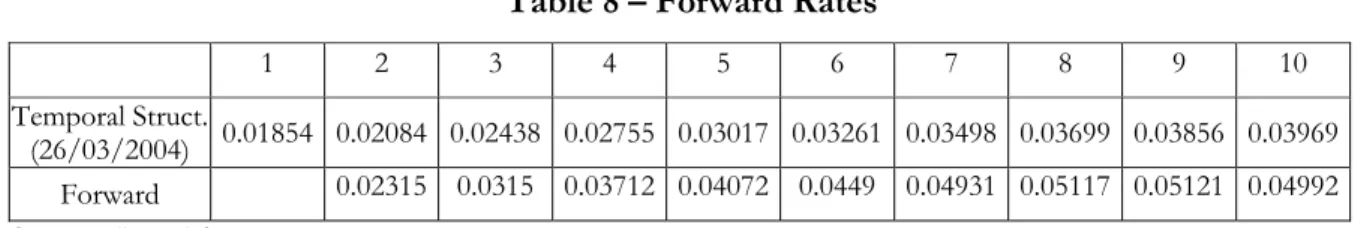
P (t, T) – the price, at moment t, of a ZCB which pays 1 monetary unit at moment T was determined based on the temporal structure of the interest rates presented in Table 8.
Table 8 – Forward Rates
1 2 3 4 5 6 7 8 9 10
Temporal Struct.
(26/03/2004) 0.01854 0.02084 0.02438 0.02755 0.03017 0.03261 0.03498 0.03699 0.03856 0.03969
Forward 0.02315 0.0315 0.03712 0.04072 0.0449 0.04931 0.05117 0.05121 0.04992
Source: Financial group.
The estimated option’s value is 1.24 percent of the invested amount. Note that this value is a conservative estimative given the assumptions of the model (for instance, we assume a flat, interest rate temporal structure, within each year, and a constant volatility parameter).
6 Average maturity of these financial contracts.
7 The volatility of the reference fund, in which are invested net premiums, is calculated using its annual net returns.
The low observed volatility of this fund (that supposedly invest in stocks, bonds, and other risky assets) can be explained by the financial group investment strategy that follows hedge funds investment principles.
8 We assume that the rational expectations theory is verified. 9 Financial product description leaflet.
3.2.2. Binomial Model
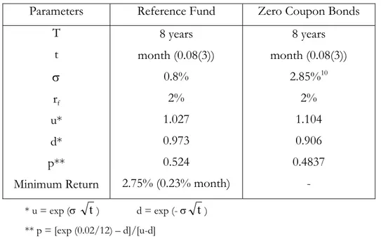
The binomial model, comparatively to the previous one, has the advantage of allowing different stochastic processes for the returns of the ZCB and the reference fund. Table 9 presents the parameters values of the binomial model.
Table 9 – Parameters of the Binomial Model
Parameters Reference Fund Zero Coupon Bonds
T t σ rf u* d* p** Minimum Return 8 years month (0.08(3)) 0.8% 2% 1.027 0.973 0.524 2.75% (0.23% month) 8 years month (0.08(3)) 2.85%10 2% 1.104 0.906 0.4837 - * u = exp (σ t ) d = exp (- σ t ) ** p = [exp (0.02/12) – d]/[u-d]
Given the assumptions for the parameters reported in Table 9, the expected present value of the ZCB is 0.84 , which corresponds to a capitalization factor of 1,19 (=1/0.84). On the other hand, the expected present value of the reference fund is 0.77, which corresponds to a capitalization factor of 1,30 (=1/0,77).
The option under evaluation is valuable only when the ZCB’s rate of return is below the one of the reference fund. Given that this is an American option, the investors return equals the maximum of the difference between the value of the ZCB and the value of the reference fund, at the moment of exercise; the value of the option if maintained alive; and zero. Within this framework, the value of the option equals 7 percent of the invested amount.
10 The volatility of the ZCB was calculated based on the monthly returns, during the period 30/12/1994 to
Still, the binomial model assumes that the ZCB’s return stochastic process follows a geometric brownian motion (GBM) (and therefore has a positive drift), when it is consensual that this process is mean reverting. In this context, the estimated value of this option is above its real value if .used a mean reverting process.
3.2.3. Monte Carlo Simulation
The Monte Carlo simulation suppresses the limitation of the binomial model, referred previously, since it allows different stochastic processes for the assets. The ZCB’s returns are modelled assuming the stochastic process defined by Vasicek (exposed in section 2),
dr = β(α - r)dt + σdWt
Considering the forward rates presented in Table 8, α equals 5 percent and β11 equals 0.0835. Given the description provided in the leaflet of the financial product, we consider that GBM is the stochastic process that best match the behaviour of the reference fund. We make use of the standard assumptions about the discrete process of the reference fund to simulate its behaviour. Therefore, we asuume time intervals of 1 month (dt = 1/12) and we use the following expression as an approximation to the evolution of its price
S(t + dt) – S(t) = µS(t)dt + σS(t)ε dt
S(t) represents the funds’ price at moment t, ε is a random number which follows a standardized normal distribution and µ is the fund’s return rate from the last period (0.25% =3%/12 months). The simulation of the fund’s price incorporates the minimum guaranteed rate of return (0.23% = 2.75% / 12 months). The simulation work involves 2,500 monthly simulations for the prices of each one of the assets through the 8 years, which implies the generation of 240,000 random numbers (2,500 iterations times 96 months) for each one of the assets.
11 We computed this value using an iterative process that minimizes the square of the difference between the
observed and the estimated interest rates temporal structure, for the time period 30/12/1994 to 26/03/2004, considering Vasicek model.
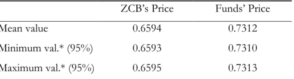
The average value of the price for each asset (table 10) is the mean of the present value of 1 monetary unit received at the end of the eighth year, discounted at the rates of return verified in each period, resulting from the 2,500 simulations. The present value of 1 monetary unit paid by the ZCB at moment T is 0.6594 m.u.., which corresponds to a capitalization factor of 1.517 (=1/0.6594). The present value of 1 m.u. paid by the reference fund at moment T is 0.7312 m.u.., which corresponds to a capitalization factor of 1.368 (=1/0.7312).
Table 10 – Assets’ Prices
ZCB’s Price Funds’ Price
Mean value 0.6594 0.7312
Minimum val.* (95%) 0.6593 0.7310
Maximum val.* (95%) 0.6595 0.7313
*Minimum value = mean value – 1.96 prices’ standard errors; Minimum value = mean value +1.96 prices’ standard errors.
Under the simulation work, the value of the option incorporated in the financial product is zero. As argued previously, the minimum rate of return guaranteed by the product only has value when the alternative investment, the ZCB, has a rate of return below the one of the reference fund. Given the assumptions, the ZCB return is never inferior to the minimum rate of return guaranteed by the product, and therefore this option is priceless.
4. Conclusions
This paper estimates the price of two different options (the surrender option and the minimum guaranteed rate of return option) provided by life insurance products, using a set of different valuation models.
Hunzinker and Koch-Medina (1996) model was used to estimate the price of the surrender option. The surrender option is worth 1.18 percent of the net premium. The minimum guaranteed rate of return option was determined in a forecasting perspective assuming stochastic interest rates. The estimated value is function of the adopted model and varies between 0 in the Monte Carlo simulation and 7 percent in the binomial model.
As a suggestion for further investigation we highlight the importance of developing a model to value both options simultaneously and the importance of these models in an accurate management of the options the insurance companies offer in their life insurance products.
5. References
Albizatti, M. O. and H. Geman (1994). Interest Rate Risk Management and Valuation of the Surrender Option in Life Insurance Policies. Journal of Risk and Insurance, 61 (4), 616-637.
Black, F. and M. Scholes (1973). The Pricing of Options and Corporate Liabilities. Journal of Political Economy, 81, 637-654.
Grosen, A. and P. L. Jorgensen (1997). Valuation of Early Exercisable Interest Rate Guarantees. The Journal of Risk and Insurance, 64 (3), 481-503.
Hull, J. C. (2000). Options, Futures and Other Derivatives. 4º ed., Prentice-Hall, Upper Saddle River.
Hunziker, J. P. and P. Koch-Medina (1996). Interest Rates and Life Insurance. In Israel Nelken, Options Embedded Bonds – Price Analysis, Credit Risk & Investment Strategies, Irwin, chapter 12, 257-271.
Margrabe, W. (1978). The Valuation of an Option to Exchange One Asset for Another. Journal of Finance, 33, 177-186
Reisman, H. (2000). Valuation of Life Insurance Contracts with Surrender Options. Davidson School of IE & Management / Technion – Israel Institute of Technology, working paper.
Smith, M. L. (1982). The Life Insurance Policy as an Options Package. Journal of Risk and Insurance, 49 (4), 583-601.
Sundaresan, S. M. (2000). Continuous-Time Methods in Finance: A Review and an Assessment. Journal of Finance, vol. LV, no. 4, 1569-1622.