Rev. bras. meteorol. vol.22 número3

(1)

ON NON-ELLIPTIC REGIONS AND SOLVABILITY OF BALANCE

EQUATIONS FOR ATMOSPHERE DYNAMICS

ANDREI BOURCHTEIN & LUDMILA BOURCHTEIN

Institute of Physics and Mathematics, Pelotas State University, Brazil

Correspondence address: Rua Anchieta 4715 bloco K, ap.304, Pelotas-RS 96015-420, Brazil

E-mail: [email protected]

Received April 2006 - Accepted July 2006

ABSTRACT

To eliminate the fast gravitational waves of great amplitude, which are not observed in the real atmosphere, the initial fi elds for numerical schemes of atmosphere forecasting and modeling systems are usually adjusted dynamically by applying balance relations. In this study we consider different forms of the balance equations and for each of them we detect the nonelliptic regions in the gridded atmosphere data of the Southern Hemisphere. The performed analysis reveals the geographical, vertical and zonally averaged distributions of nonelliptic regions with the most concentration in the tropical zone. The area of these regions is essentially smaller and less intensive for more complete and physically justifi ed balance relations. The obtained results confi rm the Kasahara’s assumption that ellipticity conditions are violated in the actual atmospheric fi elds essentially due to approximations made under deriving the balance equations.

Keywords: balance equations, initialization methods, nonelliptic regions

RESUMO: SOBRE REGIÕES NÃO ELÍPTICAS E SOLVABILIDADE DE EQUAÇÕES DE

BALANÇO PARA DINÂMICA DA ATMOSFERA.

Para eliminar as ondas gravitacionais rápidas de grande amplitude, as quais não se observam na atmosfera real, os campos iniciais para esquemas numéricos de sistemas de modelagem e previsão atmosférica são usualmente ajustados dinamicamente aplicando as relações de balanço. Neste estudo consideramos formas diferentes de equações de balanço e para cada uma dessas detectamos as regiões não elípticas nos dados atmosféricos do Hemisfério Sul. A analise realizada mostra a distribuição geográfi ca, vertical e média zonal de regiões não elípticas com maior concentração na zona tropical. A área dessas regiões é essencialmente reduzida e a intensidade é visivelmente menor para as relações de balanço mais completas e fi sicamente justifi cáveis. Os resultados obtidos confi rmam a suposição de Kasahara de que as condições de ellipticidade são violadas nos campos atmosféricos reais essensialmente devido às aproximações feitas em dedução das equações de balanço.

Palavras-chave: equações de balanço, métodos de inicialização, regiões não elípticas

1. INTRODUCTION

Numerical weather prediction, which is the core activity of atmospheric research and operational centers, consists basically of computation of solution to a set of partial differential equations expressing the conservation laws of mass, momentum and energy for compressible continuum medium in the non-inertial system related to a rotating sphere. The chosen differential model is solved numerically as initial value (or initial-boundary value) problem, requiring the defi nition

(2)

The long history of balance relations aimed to adjust the initial data may be traced back to the famous nonlinear balance equation by Charney (1955). A review of various initialization procedures, including nonlinear balance and omega equations, developed up to mid 70’s, is given by Bengtsson (1975). The current approaches to initial adjustment include nonlinear normal mode initialization (NMI) introduced by Machenhauer (1977) and Baer and Tribbia (1977), boundary derivative method (BDM) presented fi rst by Browning et al. (1980) and digital fi lter technique proposed by Lynch et al. (e.g., Lynch and Huang 1992). One of the most effective versions of the NMI is the vertical (or implicit) normal mode initialization (Bourke and McGregor 1983, Temperton 1988, Fillion and Roch 1992), which is equivalent to BDM approach (Kasahara 1982, Bijlsma and Hafkenscheid 1986, McGregor and Bourke 1988).

In his seminal paper, Daley (1981) presented the basic concepts of initialization and formulated a series of problems whose solution may improve understanding the principal properties of initialization equations. In this study we investigate one of these issues: the non-ellipticity of the balance diagnostic relations under fi xed pressure fi eld, so-called pressure (geopotential) constrained initialization. In the last years the initialization procedure was dropped in some atmospheric centers due to increased quality of observational network and objective analysis. Even having this tendency, the solution of the stated problem is important on its own because it could clarify a nature of the balance involving atmospheric fi elds.

The fi rst studies of the ellipticity conditions for balance relations were made by Charney (1955) and Houghton (1968) in the case of nonlinear balance equation on the f-plane and on the sphere. Since the last equation is the particular case of the Monge-Amper equation (Charney 1955, Kasahara 1982), these studies essentially were the applications of the well-developed theory of Monge-Ampere equation.

The first theoretical study on the non-ellipticity of simplifi ed NMI/BDM equations was presented by Tribbia (1981), who constructed theoretical example demonstrating that a certain restriction on meteorological fi elds must be satisfi ed in order to obtain a solution of the initialization system with fi xed geopotential. He used the model of isolated barotropic vorticity on the f-plane and obtained that this restriction is close to ellipticity condition of the nonlinear balance equation. The violation of ellipticity condition can lead to the divergence of the iterative method of solving the NMI/BDM equations when the height constrained initialization is required. This problem was fi rst reported by Daley (1978) when applying Machenhauer iteration procedure to the shallow water equations. The speculations about the reasons for this problem centered on two possibilities: the shortcomings of applied iterative

algorithms and the mathematical inconsistency of the boundary value problem due to existence of nonelliptic regions in the real atmospheric data (Daley 1981, Tribbia 1981, Errico 1983, Rasch 1985).

Among different studies on nonelliptic regions in the isobaric height fi elds we should note the papers by Kasahara (1982), Paegle et al. (1983) and Knox (1997), and discussion of the respective issues by Daley (1991). As it was pointed out by Kasahara (1982), in the past the occurrence of these regions used to be considered as a result of observational inaccuracies even though the changes made to recover ellipticity criterion sometimes exceeded probable data errors, specially at higher levels. Probably, Kasahara (1982) was the fi rst who stated in an explicit way that the ellipticity condition is a mathematical constraint on atmospheric fi elds, which can produce nonelliptic regions, and, consequently, impossibility of the required balance, simply because the assumptions made in deriving the balance relations could be not totally satisfi ed in real atmosphere. Therefore, one of the points of the different studies (e.g., Kasahara 1982, Paegle et al. 1983, Randel 1987 and Knox 1997) is to “adjust” ellipticity conditions by including the terms neglected in nonlinear balance relations. The new conditions, called realizability conditions, have essentially reduced the area of nonelliptic regions supporting the Kasahara’s supposition. However this approach is based on evaluation of the contribution of different terms of the primitive divergence equation for possibly recovering the ellipticity of regions rather than on the consistent system of balance relations. The only considered balance equation was the nonlinear balance equation on the f-plane or on the sphere.

In the recent years some new and more complex mathematical criterions of ellipticity have been obtained for NMI/BDM equations, which are much more general balance system based on more accurate and reliable assumptions than nonlinear balance equation (Bourchtein 2002, Bourchtein 2006). In this way, many terms neglected in the derivation of the nonlinear balance equation have been recovered in NMI/BDM equations. Therefore, one can expect that respective ellipticity conditions should be more soft and related nonelliptic regions should be more scarce in order to confi rm the Kasahara’s statement.

(3)

2. BALANCE EQUATIONS AND ELLIPTICITY CONDITIONS

In local Cartesian coordinates x, y the classic nonlinear balance equation on a tangent plane has the form (Charney 1955)

f∇2_ψ+₂

(

_{ψ ψ}_xx _yy −_ψ_xy2

)

− ∇2_Φ=₀_{, (1)}

where ψ is the streamfunction, Φ is the geopotential, f_ is a chosen value of the Coriolis parameter f, and ∇2 is the Laplace

operator. Considered as equation for the streamfunction with a given geopotential fi eld, it is a special case of Monge-Ampere equation. If this equation is to be solved on bounded domain D with imposed values of the streamfucntion on the boundary ∂D, then the problem is well posed only if the equation is of elliptic type. It requires the ellipticity condition to be satisfi ed, which has the following form for equation (1):

E₁ 2 f2 2 0

= ∇Φ+ > . (2)

Similarly, using spherical coordinates λ (longitude) and ϕ (latitude), the nonlinear balance equation assumes the form (Houghton 1968)

f

a u v u v u

∇2 +

(

−

)

− 2

2 1

ψ

ϕ λ ϕ ϕ λ β cos − ⎛ + ⎝⎜ ⎞ ⎠⎟ − ∇ = 1 0 2 2 2 a u v a

cosϕ sinϕ _ϕ Φ , (3)

where a is the Earth’s radius, f = 2Ω sin ϕ, b = 2Ω cos ϕ/ a, Ω is the angular velocity of the Earth’s rotation and u and v are the longitudinal and meridional components, respectively, of nondivergent wind, that is,

u a

= −ψϕ , v a

= ψ ϕ

λ

cos . (4)

Again, the solution of the boundary value problem for (3) with respect to the streamfunction requires the ellipticity condition, which can be written as follows (Houghton 1968):

E f u u v

a 2 2

2 2 2

2

2 0

= ∇ Φ+ +β + + > . (5)

The NMI/BDM systems have much more complex structure and contain a set of equations. For the shallow water equations on a sphere, the system contains two equations, which can be expressed in longitude-latitude coordinates (λ, ϕ) as follows (Browning et al. 1980, Bourke and McGregor 1983, Temperton 1988):

∇2 −

( )

=

(

)

2 2

Φ f curl u v, div Q Qu, v , (6)

Φ∇ − _Φ

(

2 2

)

(

( )

)

= ∇ −

(

)

2 2 2

f div u v, Q fcurl Q Qu, v , (7)

where div U V

a U V

2 1 , cos cos

(

)

= ⎡ +

(

)

⎣ ⎤⎦

ϕ λ ϕ ϕ , curl U V

a V U

2

1 ,

cos cos

(

)

= ⎡_⎣ −

(

)

⎤_⎦

ϕ λ ϕ ϕ , (8)

∇ = ⎡ +

(

)

⎣

⎢ ⎤

⎦ ⎥ 2_h 1 1

acosϕ cosϕhλλ cosϕh_{ϕ ϕ} (9) for any vector function (U, V) and any scalar function h. Here u and v are the (full) physical components of velocity, Φ_ is a mean geopotential height and Qu, Qv, QΦ contain all the

nonlinear and variable coeffi cient terms of the shallow water equations, that is,

Q u

a u

v

au a uv f f v u = − _cos_ϕ λ− ϕ+ ϕ + −

( )

1

tan ,

Q u

a v

v

av a u f f u v = − _cos_ϕ λ− ϕ+ ϕ − −

( )

1_tan 2

,

Q u

a

v

a div u v

Φ = − _cos_ϕΦλ− Φϕ−

(

Φ Φ−

)

2

( )

, .

The system (6)-(7) contains three unknown functions u, v and Φ, so it admits different closure conditions. The following natural versions of these conditions are frequently considered (Daley 1981, Daley 1991):

p≡ ∇Φ 2 −fΦ=p 0

ψ , (10)

ψ ψ= 0 , (11)

or

Φ Φ= 0 , (12)

i.e., initialization with unchanged slow mode p (frequently called unconstrained initialization), unchanged streamfunction ψ (streamfunction constrained initialization) or unchanged geopotential Φ (geopotential constrained initialization). Function p is the potential vorticity of the linearized barotropic equations on the f-plane. The nonlinear system of partial differential equations (6)-(7) with one of the closure conditions (10), (11) or (12) forms well-posed boundary value problem if it is elliptic. The ellipticity is guaranteed if its homogeneous form (characteristic determinant) is defi nite, that is, it does not change sign in the domain D of the problem.

For each of the closure conditions (10)-(12) the ellipticity criterion of the respective differential problem have been derived in Bourchtein (2002) and Bourchtein (2006). In particular, it was shown that the closures (10) and (11) generate the same ellipticity condition in the simple form

(4)

the advective speed throughout the entire domain D. Of course, this condition is satisfi ed for the barotropic model equations of the atmosphere and for the fi rst (fastest) vertical modes of a baroclinic model. However, the condition (13) is violated for very thin layers, which is the cause of the divergence of iterative algorithms applied to solve the initialization equations. Respectively, a similar behavior can be expected for slow internal modes of a baroclinic model and was observed in numerical experiments with different multilevel models reported in many papers (e.g., Daley 1981, Errico 1983, Temperton and Roch 1991).

If the geopotential constrained initialization is used, the ellipticity condition is much more complex and its approximate form in spherical coordinates can be written as follows (Bourchtein 2006):

E f u

a f v a

3

1

2 1 2 1

=⎛ − ⎝⎜

⎞

⎠⎟ + ⎛

⎝⎜ ⎞⎠⎟

cosϕ ϕ cosϕ cosϕ λ

−⎛ −

⎝⎜

⎞ ⎠⎟ >

u

a v a

λ _ϕ ϕ

1 1

0 2

cos . (14)

In the next section we show that this condition can be violated in some points of the analysis data. Even though the area covered by points with the negative values of E3 is usually small

in comparison with the total area of a chosen domain, it leads to mathematical inconsistency of the boundary value problem for considered differential equations. This inconsistency causes divergence of any iterative method applied to solve the boundary value problem. In this way, we confi rm the Daley assumption that the reason behind the problem of divergence is of mathematical nature.

3. ANALYSIS OF DISTRIBUTION OF THE NONELLIPTIC REGIONS

In this section we apply the ellipticity criteria (2), (5) and (14) to investigate the occurrence of the respective nonelliptic regions in the gridded data of the NCEP (National Centers for Environmental Prediction) analysis for the Southern Hemisphere. The data for this study were taken from the global NCEP analysis available on a spatial grid with regular latitude/ longitude resolution of 10_{and 26 vertical pressure levels. The}

analysis was restricted to the data of the Southern Hemisphere at 850, 500 and 200 hPa pressure levels for 0000 GMT 05 November 2005. The meteorological elements used are the longitudinal and meridional velocity components u and v, and the geopotential Φ.

First, we compute the ellipticity measures E1 and E2

defi ned by (2) and (5) on three chosen pressure levels. The nondivergent velocity components in (5) were evaluated by formula (4) with the streamfunction found from Poisson’s

equation ∇2_{ψ = ζ , where the Laplace operator is defi ned in (9)}

and ζ is the relative vorticity defi ned by the second formula in (8) with gridded data of the velocity components u and v. The obtained values of E2 are systematically slightly greater than

E1, but the difference is too small and can be certainly neglected

for this study. The charts of the distribution of E2 are shown

on Figs.1-6 separately for each pressure surface and Eastern and Western Hemispheres. Contour intervals are 4·10-8_s-2_{. To}

avoid the “noisy” maps, only nonelliptic regions are plotted. It can be seen the strong tendency in increasing the nonelliptic area toward higher levels. There is some relation between nonelliptic area location at different levels but it is not observed systematically. At each pressure surface the nonelliptic regions mostly appear in the tropics and subtropics, though there are some nonelliptic regions in the middle and even high latitudes as well. The geographical distribution of the nonelliptic regions in the tropics appears to be almost random. To give one example of the relation between measures E1 and E2 we also show the chart

of E1 for 500 pressure surface, Western Hemisphere (Fig.7). As

one can see the values of two measures are virtually identical for the purpose of our study. Therefore, hereafter we use only the measure E2, which is theoretically more complete.

Figure 1 – Distribution of the nonelliptic regions according to measure

E₂ in the East part of the Southern Hemisphere at 850 hPa pressure level.

Figure 2 – Same as in Figure 1, except for the West part of the Southern

(5)

Figure 3 – Same as in Figure 1, except for the 500 hPa pressure

level.

Figure 7 – Same as in Figure 4, except for the measure E1.

The following series of six charts (Figs.8-13) shows the elliptic measure E3 for corresponding surfaces and Hemispheres.

Contour intervals are 2·10-9_s-2 _{and again only the nonelliptic}

regions are plotted. On all charts for E3 the nonelliptic regions

cover signifi cantly less area and have much less intensity in comparison with the measure E2. The spatial distribution of the

nonelliptic E3 areas seems to follow the pattern of the measure

E2: these are more concentrated in tropic and subtropic zone

with rather chaotic geographical distribution and increased area and intensity at the 200 hPa pressure level.

Figure 8 – Distribution of the nonelliptic regions according to measure

E3 in the East part of the Southern Hemisphere at 850 hPa pressure

level.

Figure 9 – Same as in Figure 8, except for the West part of the Southern

(6)

level.

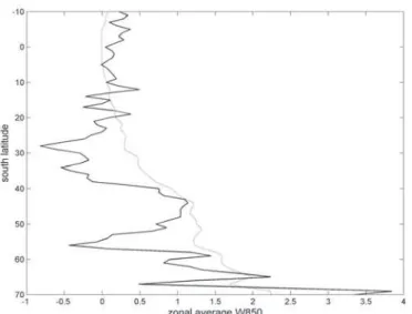
As it was pointed out by different researchers (e.g., Kasahara 1982, Knox 1997), an area average of ellipticity measure is another important index for examining the nature of nonelliptic regions. The longitudinal averages of the measures E2 and E3 are presented in Figs.14-19. The solid line is for E2

and the pointed for E3. Evidently, the negative values of E3

are much more rare and have much smaller amplitudes when compared to E2. Also, the negative values of E3 are confi ned

to very narrow tropical zone and all of them are clustered near boarder line between negative and positive values.

If we compare the results for E3 with the respective

results obtained for realizability conditions by Kasahara (1982) and Knox (1997), we can note a great similarity. Indeed, the use of ellipticity criterion E3 allows to recover ellipticity in

the major part of the negative area of the measure E2 and to

strongly decrease the remaining negative values bringing them to the boarder line. The average qualitative distribution of measure E3 exhibits the same principal characteristics as the

realizability measures, namely, the negative area is confi ned to tropic-subtropic zone and it increases toward higher pressure levels. The main difference is that the effect of the compensation of negative ellipticity achieved in Kasahara (1982) and Knox (1997) by the inclusion in the realizability conditions of additional terms from the divergence equation, is obtained in our study by substituting the ellipticity criterion for more simple balance relation by another ellipticity criterion corresponding to more complex and justifi able NMI/BDM method. In this way, we substantiate the Kasahara’s statement that ellipticity conditions can be violated in the actual atmospheric fi elds essentially due to approximations made under deriving the balance relations.

Figure 14 – The longitudinal averages of the measures E2 and E3 for

the East part of the Southern Hemisphere at 850 hPa pressure level as functions of southern latitude. The solid line is for E2 and the pointed

(7)

Figure 15 – Same as in Figure 14, except for the West part of the

Southern Hemisphere.

level.

4. CONCLUSIONS

(8)

compared with those for nonlinear balance equation. This result confi rms the Kasahara’s conclusion that the occurrence of nonelliptic regions is of physical nature and related to making simplifi cations in the derivation of the balance relations.

5. ACKNOWLEDGEMENTS

All the geographical charts were plotted with the use of free software GrADS (Grid Analysis and Display System). This research was supported by Brazilian science foundations CNPq and FAPERGS.

6. REFERENCES

Baer, F.; Tribbia, J.J. On complete fi ltering of gravity modes through nonlinear initialization. Mon. Wea. Rev., v.105, p.1536-1539, 1977.

Bengtsson, L. Four-dimensional assimilation of meteorological observations. WMO/ICSU Joint Organizing Committee, GARP Publ. Series, No.15, 1975, 76 p.

Bijlsma, S.J.; Hafkenscheid, L.M. Initialization of a limited area model: a comparison between the nonlinear normal mode and bounded derivative methods. Mon. Wea. Rev., v.114, p.1445-1455, 1986.

Bourchtein, A. Ellipticity of normal mode initialization equations. Appl. Math. Comput., v.133, p.193-211, 2002. Bourchtein, A. Ellipticity conditions of the shallow water

balance equations for atmospheric data. J. Atmos. Sci., v.63, p.1559-1566, 2006.

Bourke, W.; McGregor, T. A nonlinear vertical mode initialization scheme for a limited area prediction model. Mon. Wea. Rev., v.111, p.2285-2297, 1983.

Browning, G.L.; Kasahara, A.; Kreiss, H.-O. Initialization of the primitive equations by the bounded derivative method. J. Atmos. Sci., v.37, p.1424-1436, 1980.

Charney, J. The use of the primitive equations of motion in numerical prediction. Tellus, v.7, p.22-26, 1955.

Daley, R. Variational nonlinear normal mode initialization. Tellus, v.30, p.201-218, 1978.

Daley, R. Normal mode initialization. Rev. of Geoph. and Space Phys., v.19, p.450-468, 1981.

Daley, R. Atmospheric data analysis. Cambridge University Press, 1991, 457 p.

Errico, R.M. Convergence properties of Machenhauer’s initialization scheme. Mon. Wea. Rev., v.111, p.2214-2223, 1983.

Fillion, L.; Roch, M. Variational implicit normal mode initialization for a multilevel model. Mon. Wea. Rev., v.120, p.1051-1076, 1992.

Houghton, D.D. Derivation of the elliptic condition for the balance equation in spherical coordinates. Generalized nonlinear balance criteria and inertial stability. J.Atmos. Sci., v.25, p.927-928, 1968.

Kasahara, A. Nonlinear normal mode initialization and the bounded derivative method. Rev. of Geoph. and Space Phys., v.20, p.385-397, 1982.

Kasahara, A. Signifi cance of non-elliptic regions in balanced fl ows of the tropical atmosphere. Mon. Wea. Rev., v.110, p.1956-1967, 1982.

Knox, J.A. Generalized nonlinear balance criteria and inertial stability. J.Atmos. Sci., v.54, p.967-985, 1997.

Lynch, P.; Huang, X.-Y. Initialization of the HIRLAM model using a digital fi lter. Mon. Wea. Rev., v.120, p.1019–1034, 1992.

Machenhauer, B. On the dynamics of gravity oscillations in a shallow water model, with applications to normal mode initialization. Contrib. Atmos. Phys., v.50, p.253-271, 1977.

McGregor, T.; Bourke, W. A comparison of vertical mode and normal mode initialization. Mon. Wea. Rev., v.116, p.1320-1334, 1988.

Paegle, J.; Paegle, J.N.; Dodd, G.C. On the occurence of atmospheric states that are non-elliptic for the balance equations. Mon. Wea. Rev., v.111, p.1709-1723, 1983. Randel, W.J. The evaluation of winds from geopotential height data

in stratosphere. J. Atmos. Sci., v.44, p.3097-3120, 1987. Rasch, P.J. Developments in normal mode initialization. Part

(9)

Temperton, C. Implicit normal mode initialization. Mon. Wea. Rev., v.116, p.1013-1031, 1988.

Temperton, C.; Roch, M. Implicit normal mode initialization for an operational regional model. Mon. Wea. Rev., v.119, p.667-677, 1991.