Original Article
Designing the raw material collection system for profit maximization
under a step–price policy
Kanya Auckara-aree*
1and Rein Boondiskulchok
21 Department of Agro-Industrial Technology, Faculty of Agro-Industry,
Prince of Songkla University, Hat Yai, Songkhla, 90110 Thailand.
2 Department of Industrial Engineering, Faculty of Engineering,
Chulalongkorn University, Pathum Wan, Bangkok, 10330 Thailand.
Received 20 July 2010; Accepted 25 January 2011
Abstract
In this study, we investigate a complex situation in designing a raw material collection system, which involves collect-ion statcollect-ion locatcollect-ion, supplier selectcollect-ion, supplier–collectcollect-ion allocatcollect-ion, and transporatcollect-ion deciscollect-ions. In a raw material collectcollect-ion system, a collector has to collect more raw material quantity in order to get higher income as the price of raw material is quantity dependent. The more suppliers visit, the more income receives; however, when a collector decides to visit more suppliers, traveling distance will be longer, which will result in higher transportation costs. We formulate a Mixed Integer Programming for a location routing with setp–price policy model to find the optimal solution. The basic trade–off of the proposed model is between revenue received from totally collected quantity and total costs both fixed costs and variable costs from expanding the collection area. Instances which are created according to real–life data are applied to test the proposed model. The computational results indicate that the complex raw material collcetion system can be obtained by the proposed mathethical model. The mathematical model gives the benefit for the use of determining the optimum raw material collection system with profit maximization. The results can be used for setting up a real raw material collection system.
Keywords: location allocation, vehicle routing, profit maximization, step–price, price–quantity dependent
1. Introduction
Raw material collection systems are an important part in a supply chain of the agricultural industry where attention needs to be paid. When considering a raw material collection system in the agricultural industry, the collection process appears to be the main activity in the system. The logistics costs are a huge portion in the costs of the overall collection system. Most of the logistics costs, both fixed costs, such as collection station fixed costs, and variable costs, like trans-portation costs, rely on the operation model of a raw material
collection system. In addition to these, the agricultural industry has specific characteristics such as perishable product that affects collection time and incentive system, which influences collected quantity, which is also needed to be considered when setting up a raw material collection system.
Similar to the distribution system, the important factors in designing a raw material collection system are locating facilities, such as collection stations and factories, allocating suppliers or customers to each service area, and transport plans covering all members in the system. For the aspect of collection stations, the location and the number of collection stations are both main factors in designing the collecting system, because changing the number of collection stations affects the supply chain cost as revealed by Chopra
* Corresponding author.
(2003). In the aspect of the allocation of suppliers to collect-ion statcollect-ions, the deciscollect-ion of assigning a supplier to each collection station is the main factor to be considered in the inbound collecting system design. Suppliers should be assigned to a proper collection station. For the transporta-tion aspect, the number of suppliers selected in the route and the number of vehicles used in the routing are key factors that should be investigated for the design of an inbound collecting system. A vehicle needs to visit suppliers in the route and returns to the collection station under the capacity of the vehicle and within biological time constraints. In addi-tion to the aforesaid factors, different sets of suppliers yield difference in revenues due to price–quantity dependencies, which makes a difference in the system costs. For the supplier selection aspect, the set of suppliers selected into a raw material collection system is vital factor that should be examined. One of the practical examples is the selecting of contracted suppliers for a contract farming system. There-fore, to establish such a complicated raw material collection system, it is necessary to involve not only the location deci-sions but also the allocation decision and routing decision, which should be determined, and the supplier selection decision that should be examined as well.
An integrated problem between a location problem and a routing problem, which is such a type of problem that deals with multi–functional problems, has been widly studied in supply chain management. Many studies (Laporte, 1988; Srivastava, 1993; Min et al., 1998; Tuzun and Burke, 1999; Wu
et al., 2002; Ambrosino and Scutellà, 2005) have pointed out that the location routing problem (LRP) is defined as a vehicle routing problem in which the optimal number and locations of the depot are to be determined simultaneously with the vehicle schedules and the distribution routes so as to minimize the total costs. The location routing problem can be stated as following: given a feasible set of potential depot sites and customer sites, find the location of the depots and the routes to customers from the depots such that the overall cost of depot location and good distribution is minimized.
For the last two decades, many location allocation and vehicle routing models have been proposed (e.g. Min et al., 1998; Nagy and Salhi, 2007). Each model is characterized by the number of facilities to locate (single facility or multiple facilities), by the capacity constraints (facility capacity or vehicle capacity), by other route constraints (time windows or route lenght), and by the form of the objective function (cost minimization or profit maximization). Given a set of suppliers or customers, most studies have extensively devel-oped models so as to minimize the total system costs in the range of various complicated environments, such as multiple hierarchical structure (Ambrosino and Scutellà, 2005), multiple vehicle types (Wu et al., 2002), demand in stochastic situation (Chan et al., 2001; Liu and Lee, 2003), and planning in dynamic case (Nambiar et al., 1981; Ambrosino and Scutellà, 2005). Rarely does research address the profit maxi-mizing problem. This research model hence undertakes other viewpoints by introducing the step–price policy in the model.
With step–price environment, different quantity levels give different raw material prices. Therefore, it is essential to find a set of suppliers included in the raw material collection system. The purpose of this research is to find a solution for the problem of setting up a raw material collection system with step–price condition. With the holistic view model that considers step–price condition together with vehicle capac-ity and time duration restrictions, the optimal collection system needs to be found. The solution of the developed model is the strategy used for a raw material collection system set up by determining the location and the number of collec-tion stacollec-tions that need to be opened, a set of suppliers included into the system and the allocation of selected suppliers to each collection station, and a set of preliminary routes referring to the number of vehicles. This research emphasizes on the maximization of profit from raw material collection, which interrelates with the revenue from collected supply and total system costs.
The organization of this paper is as follows: The raw material collection system design problem with step–price policy condition is introduced in Section 2. The mathematical model formulated the investigated design problem is presented in Section 3. Some computational results are provided in Section 4. Finally, the conclusion of this study and future research development is discussed in Section 5.
2. Design Problems of a Raw Material Collection System
In view of today’s management of raw material collec-tion stacollec-tion, there are two stages of collector decision. The first stage is responsible for making set–up decisions, while the second stage is making operation decisions. For set–up decisions, the decision maker considers the location decision, supplier selection decision, allocation decision, and tran-sportation decision. Given the set–up system mechanism, the operation decision is concerned on daily implementation related to transportation decision only. It means that by given a set of open collection stations and a set of selected suppli-ers, the reassignment of routing to collect raw material is detemined. In this research, the designing of a raw material collection system in order to set up a proper collection system is studied. The collection system investigated consists of a number of suppliers, multiple collection stations with un-limited stocking area, and one factory the collected raw material has to be sent to.
supply point and the collection station, while the second one includes the transportation between the collection station and the factory.
For the first level, identical vehicles with limited material handling capacity are dispatched from a collection station to visit a set of suppliers in order to collect raw material. Each collection station has its own vehicles for the collecting from suppliers and the transportation of raw material to collection stations. When the collection process is completed, the vehicle will return to its collection station. The collected raw material is then unloaded and prepared to delivery to the factory. In the raw material collection, we assume that the supplier is visited only once by one vehicle. The number of vehicles available at each collection station is unlimited. Irrespective of the number of vehicles needed for raw material collection, the collector can support them. There is one truck per one route; therefore, the number of trucks is equal to the number of routes. The transportation here is assumed to contract to a third party for picking up the raw material. The example trucks can be rented from car rental partner. The transportation costs here include both the vehicle fixed costs and the routing costs.
For the second level, larger vehicles will transport collected raw material directly from each collection station to the factory. The transportation between the collection station and the factory is assumed to subcontract to the transporter such as a logistics partner. The transportation cost here is charged for total collected quantity delivering from each particular collection station to the factory. Figure 1 gives an illustration of the raw material collection system investigated in this research.
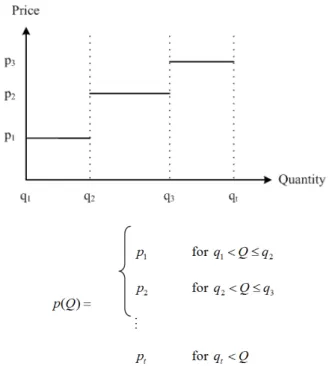
Due to relatively larger demand than supply, most factories have incentive policies for their collectors so as to facilitate more supply quantities to the factories. One of the incentive policies, which are used in a raw material collection system, is the ‘step–price policy’ as example presented in Fig-ure 2. Generally, in a collection system, the raw material price at each collection station is always based on the market price while raw material price at the factory varies according to step–price quantity levels. In this study, all collection stations pay suppliers with the same raw material price. The step–price quantity levels and step–prices offered to the collector are created by the factory. For example, if the raw material price at collection station is p0 and q* is the collected quantity, and if *
1 2
q q q then the raw material price at the factory is p1, but if q2q*q3 then the price of raw material at the factory is p2, which is equal top1 plus any incentive price. Therefore, from a collector’s viewpoint, when the buying price (p0) is fixed and the selling price per unit (step–price) is varied, a collector has to collect more raw material quantity in order to receive a higher price for the raw material at the factory.
With a step–price policy condition, it has to be a trade–off between revenue received from totally collected quantity and total costs, both fixed costs and variable costs, from expanding the collection area, if we want to get a higher
step–price level. Because each set of suppliers yields differ-ent collected quantity resulting in differdiffer-ent revenue; there-fore, the set of suppliers included in the system is an essential point for designing a raw material collection system.
Moreover, the system considered here includes time duration and vehicle capacity constraints. Since the raw material, an agricultural product, is perishable quality of raw material can decay quickly. The collection process should be kept within biological time duration relevant to the perish-ability of the raw material. Not only biological time duration but also the vehicle capacity can limit the collection process. For example, if the capacity of vehicle is full, the vehicle has to return to the collection station.
In the situation of study, no shortage or delay occurs for the collection of raw material at any supplier’s point. It is assumed that every supplier has responsibility of getting raw
Figure 1. Inbound collecting system considered in this study.
material ready for picking up at any time. Furthermore, there is no inventory consideration in this research.
Consequently, in order to maximize profit of the raw material collection system, a collector must decide where to collect raw material from and the number of suppliers, how many collection stations and where they should be located, how many vehicles in the system, and what routes each vehicle should take. A collector has to trade off between revenue from collected supply and total system costs, which include both fixed costs and variable costs, for the set–up of the raw material collection system under vehicle capacity, time duration and step–price policy circumstances.
3. Model Formulation
In the development of the location allocation and vehicle routing models, flow formulations have appeared to be the most widely used (Or and Pierskalla, 1979; Nambiar
et al., 1981; Perl and Daskin, 1985; Bookbinder and Reece,
1988; Laporte, 1988; Aykin, 1995; Hansen et al., 1994; Albareda-Sámbola et al., 2005; Ambrosino and Scutellà, 2005). Laporte (1988) has pointed out some mathematical models distinguishing between three–index and two–index location and routing flow formulations. Hansen et al. (1994) have modified the integer linear programming formulation of Perl and Daskin (1985) in order to provide an improved formu-lation, based on flow variables and flow constraints.
3.1 Mathematical model
The model investigated in this study is extended from the basic model of location allocation and vehicle routing problem by considering the selection of supplier. The aim of the model is to optimize raw material collection system in which the profit throughout the system is expected to maxi-mize. The mathematical model is developed by location and routing models mentioned in Nambiar et al. (1981), Wu et al.
(2002), and Ambrosino and Scutellà (2005). Some formula-tions are based on flow formulaformula-tions provided by Laporte (1988); furthermore, step function formulations expressed in Tsai (2007) are also added. In order to formally state the problem, the notation, which will be used throughout the paper is introduced as following:
Sets:
I represents the set of possible suppliers
J represents the set of potential collection stations
V represents the set of vehicles
T represents the set of step–prices
N represents the set of nodes, whereby N I J
Parameters:
Cj represents the fixed cost of collection station j,
j J
represents the fixed cost of vehicle used between collection station and supplier
hj represents the transportation cost per unit quan-tity between collection station j and factory, j J
rgh represents the transportation cost between node
g and node h, ,g h N
p0 represents the raw material price per unit quantity at collection station
ps represents the raw material price per unit quantity at factory at step–price s, s T
si represents the supply of supplier i, i I qs represents the minimum quantity level at step–
price s, s T
ekj represents the vehicle k set by collection station
j, k V , j J
where ekj = 1 if vehicle k is set by collection station j; otherwise ekj = 0
L represents the capacity of vehicle used between collection station and supplier
ogh represents the traveling time between node g and node h, g h N,
ai represents the loading time at supplier i, i I
B represents the biological time duration related to the perishability of raw material
Decision variables:
ys represents quantity sold at step–price s, s T
fghk represents quantity transported from node g to node h with the vehicle k, g h N, , k V
wj represents 1 if collection station j is opened, j J ; 0 otherwise
zi represents 1 if supplier i is included in the system, i I ; 0 otherwise
us represents 1 if step–price s is chosen, s T ; 0 otherwise
xghkrepresents 1 if an arc from node g to node h is on the route of vehicle k, ,g h N , k V ; 0 otherwise
The model of location allocation and vehicle routing with step–price policy problem can be formulated as follows:
0
(
s s hjk j j jhk gh ghk
s T h N j J k V j J j J h N k V g N h N k V
Max p y p f c w x r x
)
j hjk h N j J k V
h f
(1)Subject to
s i i
s T i I
y s z
(2)1
s s s s s
q u y q u s T (3)
1
s s T u
(4)hik i h N k V
x z
igk i g N k V
x z
i I (6), ,
0
ghk hgk g N g h x g N g h X
h N, k V (7), jhk kj j h N h j
x e w
j J, k V (8)jik kj i I
x e
j J, k V (9)ijk kj i I x e
j J, k V (10), gik , i gik , ihk
g N g i g N g i h N h i
f s x f
i I, k V (11), gik , ihk g N g i h N h i
f f
i I, k V (12)ghk ghk
f Lx g h N, , k V (13)
, gh ghk , i gik
g N h N h g i I g N g i
o x a x B
k V (14)0 s
y s T (15)
0 ghk
f g h N, ,k V (16)
{0,1} j
w j J (17)
{0,1} i
z i I (18)
{0,1}
s
u s T (19)
{0,1} ghk
x
g h N
,
,k V
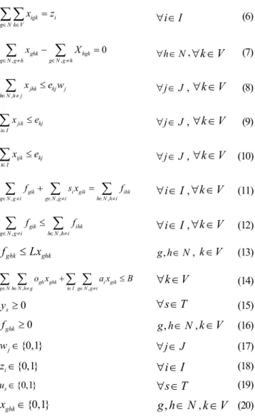
(20)The objective function (1) aims at maximizing the profit of the raw material collection system, which is the revenue from raw material collection minus the sum of raw material buying cost, collection station fixed cost, vehicle fixed cost, transportation cost between collection station and supplier, and transportation cost between collection station and factory. In constraints (2), total quantity sold at step– price s is equal to total collected quantity from selected suppliers. The constraints (3) enforce quantity sold at step– price must be in its step–price quantity level. The constraints (4) assure that only one step–price is selected. This implies that only one quantity level is chosen. To ensure only selected suppliers will be visited only once by one vehicle, the constraints (5) and (6) are added. Flow conservation constraint is expressed in constraints (7). This indicates that if a vehicle arrives at the node, it will leave that node. The constraints (8) guarantee that vehicle departs only from open collection stations. In constraints (9) and (10), a vehicle will leave and return to its own collection station. Moreover, these constraints ensure that each vehicle will leave from its own collection station mostly once. The constraints (11) state that the amount of quantity transported from the supplier is equal to the amount of quantity received by that supplier plus
its own supply. The constraints (12) represent the subtour elimination constraint. This specifies that the quantity flows out from the supplier’s point must not be lower than the quantity flows at the supplier’s point. In capacity constraints (13), the collected quantity must not be larger than the capacity of vehicle. The constraints (14) make sure that travelling time in the route of vehicle and loading time of all suppliers allocated in that route must not exceed the biologi-cal time. The constraints (15) and (16) restrict variables ys and
fghk to non–negativity. Finally, the constraints (17) to (20) force variables wj, zi, us and xghk to binary, respectively.
3.2 Numerical example
Two potential collection stations, two possible suppliers and two step–prices are provided for verifying the mathematical model (Table 1 and Table 2). To verify the mathematical model, the numerical example is solved with the use of mathematical model by the AMPL/CPLEX solver and compared to the total enumerations method, which is the solving for all possible cases of problem solution. The results from mathematical model method (Table 3) report the same optimal solution with maximum profit as received from total enumerations method (Table 4).
4. Computational Results
In this section, we solve the proposed model with the goal of computing the optimum solution. To investigate the practical complexity of the proposed model, we use test sets of 9 instances. The instances differ for the number of collec-tion stacollec-tions to locate and for the number of suppliers to select. Locations of suppliers, collection stations, and the factory are generated in uniformly distribution in the range of [0, 200]2. The number of potential collection stations and the number of possible supplier are varied from 2 to 5 and from 10 to 20, respectively. The supply from suppliers is generated in the interval [100, 250]. The fixed cost of collec-tion stacollec-tion is generated in the interval [20, 50]. The vehicle fixed cost is given at 25. The unit transportation cost between supplier and collection station is varied in 0.25, 0.5, and 1. Raw material price at collection stations and raw material step–prices at the factory are set as presented in Table 5. The capacity of each vehicle used between the supply and collection station is given a value no greater than 1, 000.
Table 1. Coordinate data used in the numerical example.
Node Coordinate X Coordinate Y
Supplier #1 1 72
Supplier #2 89 158
Collection station #1 58 89 Collection station #2 29 30
The biological time is no greater than 5, 000. Traveling time per distance is set as 1, and loading time per quantity is set as 0.025.
The Mixed Integer Programming (MIP) problem is solved by AMPL/CPLEX solver and run on PC with an Intel CorePM 2 duo 2.33 GHz CPU and 1.96 GB of RAM. For each instance, in Table 6 we report the CPU time (in seconds) and the profit of optimal solution.
Table 6 shows that the optimum solution that has been obtained from the computing. The results report that the complex raw material collcetion system can be determined by the proposed mathethical model. Nevertheless, when solving large instances, CPLEX spends the majority of its time computing, and this time grows with the size of the instances. For instance, the set of test instances 4 require 386,028.6 seconds.
Table 3. Results from the solution by the mathematical model method.
Profit = 22.183, solve time = 0.04 sec
Collection station Route Total distance Total load Total time 1 S1-1-2-S1 258.1697 415 268.5447
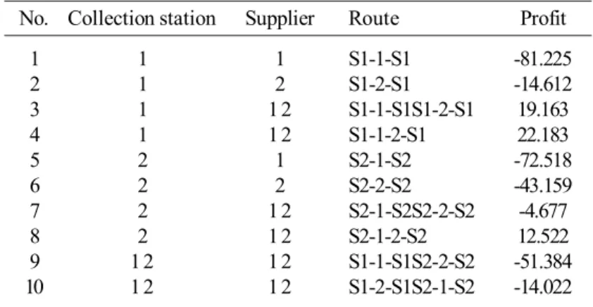
Table 4. Result from the solution by the total enumerations method.
No. Collection station Supplier Route Profit
1 1 1 S1-1-S1 -81.225
2 1 2 S1-2-S1 -14.612
3 1 1 2 S1-1-S1S1-2-S1 19.163
4 1 1 2 S1-1-2-S1 22.183
5 2 1 S2-1-S2 -72.518
6 2 2 S2-2-S2 -43.159
7 2 1 2 S2-1-S2S2-2-S2 -4.677
8 2 1 2 S2-1-2-S2 12.522
9 1 2 1 2 S1-1-S1S2-2-S2 -51.384 10 1 2 1 2 S1-2-S1S2-1-S2 -14.022 Table 2. Parameters used in the numerical example.
Parameter Unit Value
Supply of supplier #1 kg 164
Supply of supplier #2 kg 251
Fixed cost of collection station #1 Baht 42 Fixed cost of collection station #2 Baht 38 Transportation cost (Station #1 & Factory) Baht/kg 0.112712 Transportation cost (Station #2 & Factory) Baht/kg 0.111463 Transportation cost (Station & Supplier) Baht/km 0.25 Raw material cost at step–price 1 Baht/kg 2 Raw material quantity at step–price 1 kg 124.5 < Q < 207.5 Raw material cost at step–price 2 Baht/kg 2.25 Raw material quantity at step–price 2 kg 207.5 < Q Raw material buying cost at station Baht/kg 1.75 Loading time per quantity minute/kg 0.025 Traveling time per distance minute/km 1
Biological time minute 1000
Fixed cost of vehicle Baht 32
Capacity of vehicle kg 500
5. Conclusion
This research develops a mathematical model for an integrated location allocation and vehicle routing problem with step–price policy that is faced with the real–life situation in raw material collection and also useful for the operation research community. The location and the number of collec-tion stacollec-tions, a set of selected suppliers and the allocacollec-tion of selected suppliers to collection stations, as well as a set of preliminary routes referring to the number of vehicles and to maximize the profit of the system are investigated in this study. The determination of an optimum raw material collec-tion system is conducted under the consideracollec-tion of price– quantity dependence, capacity of vehicle, and collection time duration. The mathematical model is beneficial for the use of determining the optimal raw material collection system with profit maximized criterion under the extension of step–price policy environment. It can be used for both single and multiple step–prices. For single step–price, the problem will turn to minimize system cost instead of profit maximization. The collector can apply the results for setting up of a raw material collection system. Generally, the integrated location allocation and vehicle routing MIP models are very large so that solvers are incapable of obtaining optimal solution in an acceptable computational time. The model developed then might solve to optimality but consume much time. Therefore, further research is needed to extend the application of heuristic approaches, such as multi–exchange neighborhood structures, which can effectively solve larger or more real– life problems to near optimality within a reasonable computa-tional time.
References
Albareda-Sámbola, M., Díaz, J. A. and Fernández, E. 2005. A compact model and tight bounds for a combined location-routing problem. Computer & Operations Research. 32, 407-428.
Ambrosino, D. and Scutellá, M. G. 2005. Distribution network design: New problems and related models. European Journal of Operational Research. 165, 610-624. Aykin, T. 1995. The hub location and routing problem.
Euro-pean Journal of Operational Research. 83, 200-219. Bookbinder, J. H. and Reece, K. E. 1988. Vehicle routing
con-siderations in distribution system design. European Journal of Operational Research. 37, 204-213.
Chan, Y., Carter, W. B. and Burnes, M. D. 2001. A multi-depot, multi-vehicle, location-routing problem with stochas-tically processed demands. Computer & Operations Research. 28, 803-826.
Chopra, S. 2003. Designing the distribution network in a supply chain. Transportation Research Part E. 39, 123-140.
Hansen, P. H., Hegedahl, B., Hjortkjær, S. and Obel, B. 1994. A heuristic solution to the warehouse location-routing problem. European Journal of Operational Research. 76, 111-127.
Laporte, G. 1988. Location routing problems. In Vehicle Rout-ing: Methods and Studies, Golden, B. L. and Assad, A. A. editor. Elsevier Science Publishing Company, Amsterdam, Nethelands, pp 163-197.
Liu, S. C. and Lee, S. B. 2003. A two-phase heuristic method for the multi-depot location routing problem taking Table 5. Raw material price used in the study.
Level Step–price Quantity
0 (p0) 1.75 –
1 (p1) 2 30%Total Supply < Q < 50%Total Supply 2 (p2) 2.25 50%Total Supply < Q < 80%Total Supply 3 (p3) 2.4 80%Total Supply < Q
Table 6. Computational results.
Instance Collection station Supplier Profit CPU (sec)
1 2 10 731.27 11,206.9
2 2 15 1, 266.52 63,120.4 3 2 20 1, 557.64 50,168.1 4 2 25 1, 967.09 386,028.6
5 3 10 758.36 71,497.1
6 3 15 1, 228.86 78,267.8 7 3 20 1, 662.31 39,216.1
8 5 10 758.64 33,429.6
inventory control decisiond into consideration. Inter-natinal Journal of Advanced Manufacturing Techno-logy. 22, 941-950.
Min, H., Jayaraman, V. and Srivastava, R. 1998. Combined location-routing problems: A synthesis and future research directions. European Journal of Operational Research 108, 1-15.
Nagy, G. and Salhi, S. 2007. Location–routing: issues, models and methods. European Journal of Operational Research. 177, 649-672.
Nambiar, J. M., Gelders, L. F. and Van Wassenhove, L. N. 1981. A large scale location-allocation problem in the natural rubber industry. European Journal of Opera-tional Research. 6, 183-189.
Or, I. and Pierskalla, W. P. 1979. A transportation location-allocation model for regional blood banking. American Institute of Industrial Engineers Transactions. 11, 86-94.
Perl, J. and Daskin, M. S. 1985. A Warehouse location-routing problem. Transportation Research B. 19B, 381-396. Srivastava, R. 1993. Alternate solution procedures for the
location-routing problem. The International Journal of Management Sciences. 2, 497-506.
Tsai, J. -F. 2007. An optimization approach for supply chain management models with quantity discount policy. European Journal of Operational Research. 177, 982-994.
Tuzun, D. and Burke, L. I. 1999. A two-phase tabu search approach to the location routing problem. European Journal of Operational Research. 116, 87-99.