Simulating secondary organic aerosol in a regional air quality model using the statistical oxidation model – Part 2: Assessing the influence of vapor wall losses

(1)

ACPD

15, 30081–30126, 2015

Simulating secondary organic aerosol in a regional

air quality model

C. D. Cappa et al.

Title Page

Abstract Introduction

Conclusions References

Tables Figures

◭ ◮

Back Close

Full Screen / Esc

Printer-friendly Version

Interactive Discussion

Discussion

P

a

per

|

Discussion

P

a

per

|

Discussion

P

a

per

|

Discussion

P

a

per

|

Atmos. Chem. Phys. Discuss., 15, 30081–30126, 2015 www.atmos-chem-phys-discuss.net/15/30081/2015/ doi:10.5194/acpd-15-30081-2015

This discussion paper is/has been under review for the journal Atmospheric Chemistry and Physics (ACP). Please refer to the corresponding final paper in ACP if available.

Simulating secondary organic aerosol in a

regional air quality model using the

statistical oxidation model – Part 2:

Assessing the influence of vapor wall

losses

C. D. Cappa1, S. H. Jathar2, M. J. Kleeman1, K. S. Docherty3, J. L. Jimenez4, J. H. Seinfeld5, and A. S. Wexler1

1

Department of Civil and Environmental Engineering, University of California, Davis, CA, USA 2

Department of Mechanical Engineering, Colorado State University, Fort Collins, CO, USA 3

Alion Science and Technology, Research Triangle Park, NC, USA 4

Cooperative Institute for Research in Environmental Sciences and Department Chemistry and Biochemistry, University of Colorado, Boulder, CO, USA

5

(2)

ACPD

15, 30081–30126, 2015

C. D. Cappa et al.

Title Page

Tables Figures

◭ ◮

Back Close

Full Screen / Esc

Discussion

P

a

per

|

Discussion

P

a

per

|

Discussion

P

a

per

|

Discussion

P

a

per

|

Received: 21 October 2015 – Accepted: 27 October 2015 – Published: 3 November 2015

Correspondence to: C. D. Cappa (cdcappa@ucdavis.edu)

(3)

ACPD

15, 30081–30126, 2015

C. D. Cappa et al.

Title Page

Tables Figures

◭ ◮

Back Close

Full Screen / Esc

Discussion

P

a

per

|

Discussion

P

a

per

|

Discussion

P

a

per

|

Discussion

P

a

per

|

Abstract

The influence of losses of organic vapors to chamber walls during secondary organic aerosol (SOA) formation experiments has recently been established. Here, the influ-ence of such losses on simulated ambient SOA concentrations and properties is as-sessed in the UCD/CIT regional air quality model using the statistical oxidation model

5

(SOM) for SOA. The SOM was fit to laboratory chamber data both with and without ac-counting for vapor wall losses following the approach of Zhang et al. (2014). Two vapor wall loss scenarios are considered when fitting of SOM to chamber data to determine best-fit SOM parameters, one with “low” and one with “high” vapor wall-loss rates to approximately account for the current range of uncertainty in this process. Simulations

10

were run using these di_fferent parameterizations (scenarios) for both the southern Cal-ifornia/South Coast Air Basin (SoCAB) and the eastern United States (US). Accounting for vapor wall losses leads to substantial increases in the simulated SOA concentra-tions from VOCs in both domains, by factors of ∼2–5 for the low and ∼5–10 for the

high scenario. The magnitude of the increase scales approximately inversely with the

15

absolute SOA concentration of the no loss scenario. In SoCAB, the predicted SOA fraction of total OA increases from∼0.2 (no) to∼0.5 (low) and to∼0.7 (high), with the

high vapor wall loss simulations providing best general agreement with observations. In the eastern US, the SOA fraction is large in all cases but increases further when vapor wall losses are accounted for. The total OA/∆CO ratio represents dilution-corrected

20

SOA concentrations. The simulated OA/∆CO in SoCAB (specifically, at Riverside, CA) is found to increase substantially during the day only for the high vapor wall loss sce-nario, which is consistent with observations and indicative of photochemical production of SOA. Simulated O : C atomic ratios for both SOA and for total OA increase when vapor wall losses are accounted for, while simulated H : C atomic ratios decrease. The

25

(4)

ACPD

15, 30081–30126, 2015

C. D. Cappa et al.

Title Page

Tables Figures

◭ ◮

Back Close

Full Screen / Esc

Discussion

P

a

per

|

Discussion

P

a

per

|

Discussion

P

a

per

|

Discussion

P

a

per

|

possible solely through the inclusion of semi/intermediate volatility organic compounds in the simulations. These results overall demonstrate that vapor wall losses in cham-bers have the potential to exert a large influence on simulated ambient SOA concen-trations, and further suggest that accounting for such effects in models can explain a number of di_fferent observations and model/measurement discrepancies.

5

1 Introduction

Particulate organic matter, or organic aerosol (OA), is derived from primary emissions or from secondary chemical production in the atmosphere from the oxidation of volatile organic compounds (VOCs). OA makes up a substantial fraction of atmospheric sub-micron particulate matter (Zhang et al., 2007), influencing the atmospheric fate and

10

impact of PM on regional and global scales. Gas-phase oxidation of VOCs leads to the formation of oxygenated product species that can condense onto existing particles or nucleate with other species to form new particles (e.g. Ziemann and Atkinson, 2012). Much of the understanding regarding the formation of secondary organic aerosol (SOA) via condensation has been derived from experiments conducted in laboratory

cham-15

bers. In a typical experiment, a precursor VOC is added to the chamber and exposed to an oxidant (e.g OH, O₃or NO₃). As both the precursor VOC and the oxidation prod-ucts react with the oxidant, SOA is formed. The amount of SOA formed per amount of precursor reacted (i.e. the SOA mass yield) can then be quantified (e.g. Odum et al., 1996). Such SOA yield measurements form the basis of most parameterizations of

20

SOA formation in regional air quality and global chemical-transport and climate models (Tsigaridis et al., 2014). However, too often simulated SOA concentrations underesti-mate observed values, especially in polluted regions, and sometimes dramatically so (Heald et al., 2005; Volkamer et al., 2006; Ensberg et al., 2013). There have been var-ious efforts to account for model/measurement disparities including, most notably: (i)

25

(5)

ACPD

15, 30081–30126, 2015

C. D. Cappa et al.

Title Page

Tables Figures

◭ ◮

Back Close

Full Screen / Esc

Discussion

P

a

per

|

Discussion

P

a

per

|

Discussion

P

a

per

|

Discussion

P

a

per

|

as semi-volatile (Robinson et al., 2007), (ii) the addition of ad hoc “ageing” schemes on top of existing parameterizations of SOA from VOCs (Lane et al., 2008b; Tsimpidi et al., 2010; Dzepina et al., 2011), (iii) updating of aromatic SOA yields (Dzepina et al., 2009), and (iv) production of SOA in the aqueous phase in aerosol-water, clouds and fogs (Ervens et al., 2011). More recently, concerns over the influence of vapor wall

5

losses on the experimental chamber data used to develop the parameterizations have arisen (Matsunaga and Ziemann, 2010; Zhang et al., 2014). The influence of erro-neously low SOA yields due to vapor wall losses on simulated SOA concentrations in three-dimensional regional models and properties is the focus of the current work.

Recent observations have demonstrated that organic vapors can be lost to Teflon

10

chamber walls, and that the extent of loss is related to the compound vapor pressures (Matsunaga and Ziemann, 2010; Kokkola et al., 2014; Krechmer et al., 2015; Yeh and Ziemann, 2015; Zhang et al., 2015). These results suggest that vapor wall losses dur-ing SOA formation experiments could potentially bias observed SOA concentrations. Indeed, Zhang et al. (2014) observed that SOA yields from toluene₊OH

photooxida-15

tion depend explicitly on the seed particle surface area, all other conditions being equal. They interpreted these observations using a dynamic model of particle growth coupled with a parameterizable gas-phase chemical mechanism, the statistical oxidation model (SOM) (Cappa and Wilson, 2012). They determined that substantial vapor wall losses were most likely the cause of this dependence, with biases of up to a factor of ∼4

20

for these experiments. Further, they estimated for this system that the vapor wall loss rate coefficient (k_wall) was ∼2×10−4s−1 for their 25 m3 chamber. This value of k_wall

is in reasonable agreement both with theoretical expectations – so long as the vapor-wall accommodation coe_fficient (α_wall) is >10−5 _{– and with results of Ziemann and}

colleagues (Matsunaga and Ziemann, 2010; Yeh and Ziemann, 2015) who estimated

25

kwall∼6×10

−4

s−1 for their 8 m3 chamber. Kokkola et al. (2014) have also suggested vapor wall losses can impact SOA yields, although they determined a much largerk_wall

(6)

ACPD

15, 30081–30126, 2015

C. D. Cappa et al.

Title Page

Tables Figures

◭ ◮

Back Close

Full Screen / Esc

Discussion

P

a

per

|

Discussion

P

a

per

|

Discussion

P

a

per

|

Discussion

P

a

per

|

suggest thatk_wallcan vary by an order of magnitude (∼2×10−6–3×10−5s−1) and that

k_wall is dependent on the OVOC vapor pressure (Zhang et al., 2015); such low k_wall

values implies that theαwall is<10

−5

and controls the rate of vapor loss to the walls. Although the exact value ofk_wall is likely chamber-specific (which likely contributes to some of the above-mentioned variability in k_wall) and thus the exact influence of

5

vapor wall losses on chamber SOA measurements remains somewhat uncertain, the preponderance of evidence suggests that such e_ffects are important. Existing SOA pa-rameterizations have typically not been determined with explicit accounting for vapor wall losses. Consequently, they likely underestimate actual SOA formation in the atmo-sphere where walls are much less important (although dry deposition of vapors may

10

still be a factor, Hodzic et al., 2014). Two recent efforts have attempted to estimate the influence of vapor wall losses on SOA concentrations in the atmosphere (Baker et al., 2015; Hayes et al., 2015). One of the studies (Baker et al., 2015) builds on the existing two-product parameterization of SOA formation in the Community Multiscale Air Quality (CMAQ) model and simply scales the yields of the semi-volatile products up by factors

15

of 4. In the two-product model, a given VOC reacts to form two semi-volatile prod-ucts that partition to the condensed phase. The semi-volatile prodprod-ucts are formed with mass yields,y_i, and partitioning coefficients, K_i, that have been determined by fitting the model to data from chamber experiments in which vapor wall losses were not ac-counted for. The other study (Hayes et al., 2015) used a similar yield-scaling approach,

20

but within the volatility basis set (VBS) four-product framework to represent SOA for-mation, and they scaled the mass yields for only the semi-volatile product species from aromatics. Not surprisingly, these simple ad hoc scaling methods demonstrated that increasing the yields of the semi-volatile products from their originally parameterized values increases the simulated SOA concentration, but quantitative interpretation of the

25

(7)

va-ACPD

15, 30081–30126, 2015

C. D. Cappa et al.

Title Page

Tables Figures

◭ ◮

Back Close

Full Screen / Esc

Discussion

P

a

per

|

Discussion

P

a

per

|

Discussion

P

a

per

|

Discussion

P

a

per

|

por wall losses on simulated SOA concentrations in regional air quality models is thus needed.

In this study, the SOM SOA model (Cappa and Wilson, 2012) is utilized to examine the influence of vapor wall losses on simulated SOA concentrations and O : C atomic ratios in a 3-D regional air quality model, specifically the UCD/CIT (Kleeman and Cass,

5

2001). What distinguishes the present approach is that the potential influence of vapor wall losses is inherently accounted for during the development of the SOM SOA pa-rameterization (Zhang et al., 2014). This can be contrasted with a simple scaling of an existing parameterization. The current approach allows for more detailed characteriza-tion of different precursor species, reaction conditions (e.g. NO_x sensitivities) and the

10

complex interplay of various timescales (reaction, gas/wall partitioning and gas/particle partitioning). This also allows for examination of the extent to which different assump-tions regarding the value of k_wall (i.e. the first-order rate constant for vapor loss to chamber walls) during development of the SOA parameterization impact simulations of ambient SOA concentrations. Further, the SOM framework simulates O : C atomic

15

ratios in addition to OA mass concentrations, and thus allows for more detailed assess-ment of the simulated OA and comparison with observations. Our results demonstrate that accounting for vapor wall losses can have a substantial impact on simulated SOA concentrations and suggest that there may be regionally-specific differences.

2 Methods

20

2.1 Air quality model

Regional air quality simulations were performed using the UCD/CIT chemical transport model (Kleeman and Cass, 2001) for two geographical domains: (i) the Southern Cali-fornia Air Basin (SoCAB) and (ii) the eastern US. Details regarding the general model configuration and emissions inventory used have been previously discussed (Jathar

25

(8)

ACPD

15, 30081–30126, 2015

C. D. Cappa et al.

Title Page

Tables Figures

◭ ◮

Back Close

Full Screen / Esc

Discussion

P

a

per

|

Discussion

P

a

per

|

Discussion

P

a

per

|

Discussion

P

a

per

|

specific to the current work are provided in the following sections. Model simulations were run for SoCAB from 20 July to 2 August 2005 and for the eastern US from 20 Au-gust to 2 September 2006. Model spatial resolution was higher in SoCAB (8 km×8 km) than in the eastern US (36 km×36 km) to account for the different domain sizes.

2.2 Statistical oxidation model for SOA

5

SOA formation from six VOC classes was simulated using the statistical oxidation model (Cappa and Wilson, 2012; Cappa et al., 2013), which was recently imple-mented in the UCD/CIT model (Jathar et al., 2015a). The VOC classes considered are: long alkanes, benzene, high-yield aromatics (i.e. toluene), low-yield aromatics (i.e. m-xylene), isoprene and terpenes (including both mono- and sesquiterpenes). SOM is

10

a parameterizable model that simulates the multi-generational oxidation of the product species formed from reaction of the SOA precursor VOCs. In SOM, a “species” is de-fined as a molecule with a specific number of carbon and oxygen atoms (N_Cand N_O, respectively), and where the VOC-specific properties of these SOM species are deter-mined through fitting to laboratory observations. Reactions of a SOM species lead to

15

either functionalization (i.e. addition of oxygen atoms while conserving the number of carbon atoms) or fragmentation (i.e. the production of two species which individually have fewer carbon atoms but where the total carbon is conserved, and where each new species adds one additional oxygen atom). The particular tunable parameters in SOM are: the probability of adding one, two, three or four oxygen atoms per reaction,

20

referred to asp_XO; the decrease in vapor pressure per added oxygen, referred to as

∆LVP; and the probability of fragmentation, which is related to the O : C atomic ratio of a given species as P_frag=(O : C)mfrag _{and where} _m

frag is the tunable parameter. SOA

formation from the semi-volatile SOM species assumes that partitioning is described according to absorptive particle partitioning theory (Pankow, 1994), and the

gas-25

(9)

ACPD

15, 30081–30126, 2015

C. D. Cappa et al.

Title Page

Tables Figures

◭ ◮

Back Close

Full Screen / Esc

Discussion

P

a

per

|

Discussion

P

a

per

|

Discussion

P

a

per

|

Discussion

P

a

per

|

conducted in the Caltech chamber both with and without accounting for vapor wall losses during the fitting process (discussed further below); references for the specific experiments considered are provided in Table S1 in the Supplement. The specific in-fluence of considering multi-generational ageing on simulated SOA concentrations and properties is discussed in a companion paper (Jathar et al., 2015b).

5

2.3 Accounting for vapor wall loss

2.3.1 SOM

Vapor wall losses have been accounted for using SOM, as detailed in Zhang et al. (2014). Vapor wall loss is treated as a reversible, absorptive process with va-por uptake specified using a first-order rate coefficient (kwall) and the desorption rate 10

related to the e_ffective saturation concentration,C∗, of the organic species and the ef-fective absorbing mass of the walls (Matsunaga and Ziemann, 2010). Unique SOM fits (i.e. values ofmfrag,∆LVP andpXO) have been determined for different assumed values

ofk_wall. Best-fit values are provided in Table S1. It should be noted that the influence of vapor wall losses is inherent in the fit parameters, and in the absence of walls (i.e. in the

15

atmosphere) the predicted SOA formed will be larger when the fits account for vapor wall losses. Here, values of k_wall=0, 1×10−4s−1 and 2.5×10−4s−1 are considered,

corresponding to a base case with no vapor wall losses assumed during fitting (SOM-no), a low vapor wall loss case (SOM-low) and high vapor wall loss case (SOM-high), respectively. The non-zero values of k_wall are chosen to be consistent with previous

20

observations (Zhang et al., 2014) and approximately reflect the range of uncertainty. An important aspect of vapor wall loss is that the impact it has on SOA concentra-tions is dependent upon the timescale associated with vapor-particle equilibration (τ_v-p) (McVay et al., 2014; Zhang et al., 2014). Theτ_v-pis related to the accommodation coef-ficient associated with vapor condensation on particles,α_particle. Above a vapor-particle

25

accommodation coe_fficient ofα_particle∼0.1 variations in the exact value ofα_particledoes

(10)

ACPD

15, 30081–30126, 2015

C. D. Cappa et al.

Title Page

Tables Figures

◭ ◮

Back Close

Full Screen / Esc

Discussion

P

a

per

|

Discussion

P

a

per

|

Discussion

P

a

per

|

Discussion

P

a

per

|

have no influence on the amount of SOA formed whenαparticle≥0.1, only that the net

impact does not depend on α_particle. Below this value, vapor-particle equilibration is slowed and the effects of loss of vapors to the walls are accentuated. Thus, a conser-vative estimate of the influence of vapor wall losses on SOA formation is obtained using

α_particle≥0.1. Here, data fitting and parameter determination was performed assuming

5

that α_particle=1, and is thus a conservative estimate. SOM was fit to SOA formation

experiments conducted in the California Institute of Technology chamber, following the methodologies described in Cappa et al. (2013) and Zhang et al. (2014). Observed suspended particle concentrations have been corrected only for physical deposition on chamber walls, which is appropriate since vapor wall losses are accounted for

sepa-10

rately by SOM. Best-fit values for the SOM parameters for the base case are given in Jathar et al. (2015a) and values for SOM-low and SOM-high determined here are given in Table S1, along with the sources of the experimental data. Parameters have been separately determined for experiments conducted under low-NO_x and high-NO_x con-ditions since the SOA yields di_ffer. Example results that illustrate the influence of vapor

15

wall losses on simulated SOA yields are presented in Fig. S1 in the Supplement for box model simulations that have been conducted using the best-fit parameters determined for toluene SOA (low-NO_x conditions), but where the simulations are run assuming there are no walls (i.e. by settingk_wall=0).

2.3.2 Two-product model

20

Ideally, SOA levels from the SOM-based simulations can be compared with similar re-sults based on the commonly used two-product model. To do so involves determining new parameters for the two-product model in which vapor wall losses are explicitly accounted for. Therefore, vapor wall-loss corrected SOA yield curves (i.e. [SOA] vs. [_∆HC], where _∆HC is the concentration of reacted hydrocarbon) were generated with

25

(11)

ACPD

15, 30081–30126, 2015

C. D. Cappa et al.

Title Page

Tables Figures

◭ ◮

Back Close

Full Screen / Esc

Discussion

P

a

per

|

Discussion

P

a

per

|

Discussion

P

a

per

|

Discussion

P

a

per

|

and partitioning coefficients. These new fits would inherently account for the influence of vapor wall loss since the two-product model is being fit to the corrected “wall-less” data and thus differ from ad hoc scaling of yields. However, it was determined that the two-product fits were not sufficiently robust across the entire suite of compounds and vapor wall loss conditions considered to be implemented in the atmospheric model. An

5

example for SOA from dodecane+OH under low-NO_x reaction conditions is shown in Fig. S2 in the Supplement. We have determined that this lack of robustness is a result of the limited dynamic range of the 2-product model. More specifically, the SOA concen-trations from the chamber observations, both uncorrected and corrected, ranged from

∼1–500 µg m−3, often with few data points at concentrations less than ∼10 µg m−3.

10

Thus, when fits were performed, inconsistent behavior between the di_fferent vapor wall loss conditions was obtained over the atmospherically relevant concentration range (∼0.1–20 µg m−3). Attempts were made to fit the two-product model over a restricted

concentration range or to fit using log([SOA]) instead of [SOA]. However, neither e_ffort led to su_fficiently robust results (although both did lead to improvements). This null

re-15

sult suggests that simple scaling of two-product yields (Baker et al., 2015) to account for the e_ffects of vapor wall losses may not be appropriate. This may similarly apply to scaling of VBS parameters (Hayes et al., 2015), although the greater flexibility of the VBS (commonly implemented with four products, instead of two) can potentially allow for unique “wall-less” fits to be determined (Hodzic et al., 2015). The extent to which

20

such alternative methods can robustly account for vapor wall losses that are computa-tionally less intensive than SOM will be explored in future work.

2.4 Primary organic aerosol and IVOCs

Primary organic aerosol (POA) derived from anthropogenic (e.g. vehicular activities, food cooking) or pyrogenic (e.g. wood combustion) sources are simulated assuming

25

(12)

ACPD

15, 30081–30126, 2015

C. D. Cappa et al.

Title Page

Tables Figures

◭ ◮

Back Close

Full Screen / Esc

Discussion

P

a

per

|

Discussion

P

a

per

|

Discussion

P

a

per

|

Discussion

P

a

per

|

a semi-volatile framework (Robinson et al., 2007), such that some fraction of the POA can evaporate (i.e. SVOCs) and react within the gas-phase and be converted to SOA (sometimes improperly referred to as “oxidized POA”), then the amount of POA would likely decrease (due to evaporation) and the amount of simulated SOA would increase (due to condensation of oxidized SVOC vapors); the total OA concentration

5

(POA+SOA) may or may not increase as a result, depending on the details of the parameterization and the atmospheric conditions. Additionally, nearly all modeling ef-forts in which POA is treated as semi-volatile have also included contributions from gas-phase IVOCs as an added class of SOA precursors; these two issues are rarely implemented independently in models, although their contributions can be separately

10

tracked. Whereas simply treating POA as semi-volatile may or may not lead to an in-crease in the total OA concentration, the introduction of new SOA precursor mass in the form of IVOCs will inevitably lead to production of more SOA in the model. The relative importance of IVOCs will depend on the amount of added IVOC mass and the propensity of these IVOC vapors to form SOA in the model (i.e. their e_ffective SOA

15

yield). In the current study, we do not explicitly consider the potential for IVOCs to con-tribute to the ambient SOA burden, focusing instead on how vapor wall losses influence SOA formation from VOCs. We will aim to consider contributions from IVOCs and how they are influenced by vapor wall losses in future studies. Regardless, the implications of our particular treatment (non-volatile POA excluding IVOCs) are discussed below.

20

2.5 Model simulations and outputs

Six individual model simulations have been carried out to determine the spatial distribu-tion of SOA concentradistribu-tions. Each simuladistribu-tion used one of the SOM parameterizadistribu-tions, i.e. SOM-no, SOM-low or SOM-high with either the low- and high-NO_xparameters. Be-sides the absolute SOA concentration, SOM also allows for explicit calculation of the

25

average (and precursor-specific) O : C and H : C atomic ratios and of the SOA volatil-ity distribution, which characterizes the distribution of particulate and gas-phase mass concentrations with respect toC∗

(13)

ACPD

15, 30081–30126, 2015

C. D. Cappa et al.

Title Page

Tables Figures

◭ ◮

Back Close

Full Screen / Esc

Discussion

P

a

per

|

Discussion

P

a

per

|

Discussion

P

a

per

|

Discussion

P

a

per

|

it is assumed that the non-volatile POA has a constant O : C=0.2 and H : C=2.0 (Ng et al., 2011). Since the simulated (O : C)_total is just a combination of (O : C)_SOA and (O : C)_POA, assuming a different value for (O : C)_POA would change the absolute value of (O : C)_totalbut not any dependence on simulation conditions. This is similarly true for (H : C)_total.

5

As noted above, unique sets of SOM parameters were fit to experiments conducted under either low- or high-NO_x conditions assuming a particular value for k_wall. Since each simulation used a single set of SOM fit parameters (e.g. SOM-no fit to low-NO_x experiments) the SOA NO_xparameterization used in a given simulation is independent of the actual simulated ambient NO_x concentrations or NO/HO₂ ratio. Consequently,

10

comparison between the simulations conducted using the low- and high-NO_x param-eterizations gives an indication of the range expected from variability in NO_x levels, and the average between the two simulations provides a representation that is inter-mediate between these two extremes. Unless otherwise specified, reported values are for the average of the simulations run using the low- and high-NO_x parameterizations.

15

This approach towards understanding the influence of NO_x is different than some pre-vious approaches that attempted to account for the SOA NO_x dependence in a more continuously variable manner. For example, some simulations using the two-product approach have used the instantaneous NO/HO₂ratios predicted by the model to allow distinguishing between low- and high-NO_xproducts and SOA yields for aromatic VOCs

20

(Carlton et al., 2010). Similarly, instantaneous VOC/NO_x ratios have been used with VBS-type models for aromatic VOCs to allow for interpolation between the two regimes (Lane et al., 2008a). Typically, these e_fforts have not considered the NO_x-dependence of monoterpene and sesquiterpene yields even though it is experimentally established that the NO_xcondition (and more specifically, the NO/HO₂ratio) influences SOA yields

25

(14)

ACPD

15, 30081–30126, 2015

C. D. Cappa et al.

Title Page

Tables Figures

◭ ◮

Back Close

Full Screen / Esc

Discussion

P

a

per

|

Discussion

P

a

per

|

Discussion

P

a

per

|

Discussion

P

a

per

|

Further, modeled NO/HO₂ ratios may be o_ffby orders of magnitude, most likely due to poor representation of HO₂ concentrations (Carlton et al., 2010), making it difficult to understand how well the conditions of the laboratory translate to the model envi-ronment. By considering the low- and high-NO_x parameterizations separately, i.e. the approach used in the current study, bounds on the overall influence of NO_x on the

5

simulated SOA can be established. However, this approach will not capture how the simulated SOA may vary due to spatial and temporal variations in the model NO_x and oxidant fields. Future e_fforts will aim to account for the NO_x-dependence of SOA for-mation in a more continuously varying manner, and to account for recent updates to the detailed isoprene oxidation mechanism (Pye et al., 2013).

10

3 Results and discussion

3.1 General influence of vapor wall loss on simulated SOA

The spatial distribution of the SOM-no model SOA concentrations is shown for SoCAB and the eastern US using the average from the simulations carried out using the low-and high-NO_xparameterizations (Fig. 1a and b). (Again, the low- and high-NO_x

desig-15

nations here refer only to the experimental conditions under which the SOM parameters were determined, not the actual NO_x conditions in the UCD/CIT model.) For SoCAB, predicted SOA concentrations are largest in and around downtown Los Angeles and in the forested regions of the Los Padres National Forest and the Santa Monica Moun-tains National Recreation Area in the NW quadrant. The spatial distribution of SOA

20

is similar to that obtained using the conventional two-product SOA parameterization (Jathar et al., 2015a, b). For the eastern US, predicted SOA concentrations are largest in the southeast, in particular around Atlanta, Georgia. Overall, the simulated SOA concentrations with the SOM-no model are larger in the eastern US than in SoCAB, reflecting the relatively strong influence of biogenic emissions in this region.

(15)

ACPD

15, 30081–30126, 2015

C. D. Cappa et al.

Title Page

Tables Figures

◭ ◮

Back Close

Full Screen / Esc

Discussion

P

a

per

|

Discussion

P

a

per

|

Discussion

P

a

per

|

Discussion

P

a

per

|

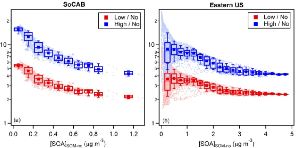
The influence of vapor wall losses on the simulated ambient SOA concentrations is illustrated in Fig. 1c–f as the ratio between the SOA from the low and SOM-high simulations to the SOM-no (no wall losses) simulation. This ratio will be referred to generally as the wall loss impact (Rwall, low orRwall, high). Values ofRwall larger than

one indicate that accounting for vapor wall losses as part of the SOM parameterization

5

leads to an increase in the predicted SOA concentrations. In the SoCAB, theR_{wall, low}

varies from 1.5–4.5, while theR_{wall, high}varies from 3 to more than 10. The largest ratios (indicating the largest impact of accounting for vapor wall losses) tend to occur in more remote locations as this is where concentrations are lower (Fig. 2). However, the impact is still large in downtown Los Angeles and the greater LA region (averageR_{wall, low}∼2.5

10

and R_{wall, high}∼5). In the eastern US, the simulated R_wall vary over a similar range

as in SoCAB, with R_{wall, low} varying from 1.5–5 and R_{wall, high} from 3 to 10. There is again a general, although not exact, inverse relationship betweenR_wall and the abso-lute SOA concentrations; the greater scatter in the eastern US compared to SoCAB at low SOA concentrations likely reflects the larger spatial range considered. The

small-15

est simulated R_wall values occur across the southeast and up the eastern seaboard (R_{wall, low}∼2.5 andR_{wall, high}∼5) while the largest values occur over the Great Lakes

and Michigan, Nebraska, and the Gulf of Mexico and Atlantic Ocean; there is a steep increase going from land to sea.

Regional air quality models have historically overestimated the urban-to-regional

gra-20

dient in total OA concentrations. Robinson et al. (2007) showed that the simulated urban-to-regional gradient could be reduced and made more consistent with observa-tions by treating POA as semi-volatile and adding SVOCs and IVOCs as SOA-forming species. The current results suggest a complementary explanation, namely that the urban-to-regional gradient can be reduced when vapor wall losses are accounted for

25

since Rwall generally decreases with SOA concentration and since POA is identical

(16)

ACPD

15, 30081–30126, 2015

C. D. Cappa et al.

Title Page

Tables Figures

◭ ◮

Back Close

Full Screen / Esc

Discussion

P

a

per

|

Discussion

P

a

per

|

Discussion

P

a

per

|

Discussion

P

a

per

|

coast of LA (regional) and downtown LA (urban) decreases from 2.3 (SOM-no) to 1.5 (SOM-low) to 1.3 (SOM-high), for example. Additionally, it has been suggested that the typical underprediction of SOA by air quality and chemical transport models might increase with photochemical age (Volkamer et al., 2006). The current results suggest the possibility that SOA concentrations in more remote (lower concentration) regions

5

may be underestimated in models to a greater extent than in high-source (higher con-centration) regions due to a lack of accounting for vapor wall losses.

3.2 OA composition and concentrations

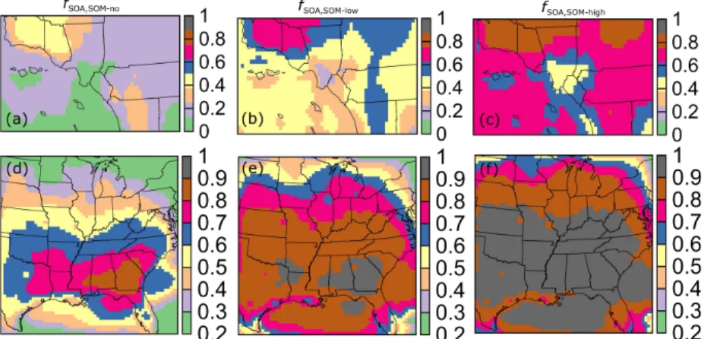
The simulated fraction of total OA that is SOA (f_SOA) is substantially smaller in SoCAB than in the eastern US, especially the southeast US (Fig. 3). The predictedf_SOAvalues

10

vary spatially within a given region, with the SOM-no simulations in the general range of∼0.1–0.3 for SoCAB and∼0.4–0.9 for the eastern US. This di_fference between

re-gions results from the substantial POA emissions in SoCAB and the large emissions of biogenic VOCs across the southeast US. Consequently, accounting for vapor wall losses has a larger impact on the absolute total OA (SOA₊POA) concentrations in the

15

eastern US than it does in SoCAB, although the impact in both regions is substantial. For SoCAB, the predicted 24 h averagef_SOA range increases to ∼0.2–0.5 for

SOM-low and to∼0.4–0.8 for SOM-high simulations. These model results can be compared

with measurements from the 2005 SOAR field study in Riverside, CA, which overlaps with the simulation period. The observedf_SOAduring SOAR ranged from∼0.6 in early

20

morning to∼0.9 in midday, with a campaign-average of∼0.78 (Docherty et al., 2011).

Measurements at Pasadena, CA during a later time period, June 2010 during the Cal-Nex study, give similar results with the campaign-average f_SOA=0.6 (Hayes et al., 2013). (Note that here we are equating SOA with the “oxygenated organic aerosol”, or OOA factors that are obtained from positive matrix factorization of the measured OA

25

(17)

ACPD

15, 30081–30126, 2015

C. D. Cappa et al.

Title Page

Tables Figures

◭ ◮

Back Close

Full Screen / Esc

Discussion

P

a

per

|

Discussion

P

a

per

|

Discussion

P

a

per

|

Discussion

P

a

per

|

For the eastern US, the predictedfSOArange increases from 0.4–0.9 for SOM-no to

∼0.7–0.9 for SOM-low and to∼0.8–1 for SOM-high. These predicted values can be

compared with measurements made at a few locations in the southeastern US (specif-ically, sites in Alabama and Georgia), which show that thefSOA in this region exhibits

a strong seasonal dependence and some spatial variation (Xu et al., 2015b). The

mea-5

surements in spring and summer indicate that the total OA is dominated by SOA, with

f_SOAmeasurements ranging from 0.7 to 1 and with the smaller values observed at the more urban sites. The predictedf_SOAfrom the SOM-low and SOM-high simulations are most consistent with this range, with thef_SOA from the SOM-no simulations being on the low side, especially in comparison with the more rural sites.

10

The simulated total OA concentrations are compared to ambient OA measurements made at the STN (Speciated Trends Network) and IMPROVE (Interagency Monitoring of Protected Visual Environments) (The Visibility Information Exchange Web System (VIEWS 2.0), 2015) air quality monitoring sites in SoCAB and the eastern US; the regional di_fferences in f_SOA should be kept in mind for this model/measurement

com-15

parison. A map of sites is shown in Fig. S3 in the Supplement. STN sites tend to be more urban and have higher OA concentrations compared to IMPROVE sites, which tend to be more remote. OA concentrations are estimated as the measured organic car-bon (OC) concentrations times 2.1 for IMPROVE sites and as 1.6×([OC]−0.5 µg m−3)

for STN sites (Turpin and Lim, 2001). The−0.5 µg m−3o_ffset for the STN sites arises

20

because the IMPROVE data are both artifact and blank corrected while the STN data are only artifact corrected (Subramanian et al., 2004). The difference in scaling factors (2.1 vs. 1.6) approximately accounts for di_fferences in the OA/OC conversion between more urban and more rural networks (Turpin and Lim, 2001). Given the generally re-gional character of OA in much of the eastern US, it may be that the difference in

25

(18)

ACPD

15, 30081–30126, 2015

C. D. Cappa et al.

Title Page

Tables Figures

◭ ◮

Back Close

Full Screen / Esc

Discussion

P

a

per

|

Discussion

P

a

per

|

Discussion

P

a

per

|

Discussion

P

a

per

|

Table 1 lists statistical metrics of fractional bias and normalized mean square er-ror (NMSE) that capture model performance for OA for all simulations for both do-mains across the STN and IMPROVE monitoring networks. Scatter plots are shown in Figs. S4 and S5 in the Supplement; many more sites are considered in the eastern US than in the SoCAB given the larger geographical domain and distribution of sites. In

5

both regions, the SOM-no simulations underpredict the STN and IMPROVE observa-tions, especially in the SoCAB. The negative bias of the SOM-no simulations is gener-ally improved as vapor wall losses are accounted for. For both the STN and IMPROVE sites in the SoCAB the SOM-high simulations give best agreement. For the eastern US STN sites, an average of the SOM-low and SOM-high simulations provides the best

10

agreement. For the eastern US IMPROVE sites, the SOM-low simulations provide the best agreement, although with some overprediction. (If the eastern US STN and IM-PROVE measurements do underestimate the actual OA concentrations, the degree to which accounting for vapor wall losses improves the model-measurement comparison will increase.) The simulated anthropogenic/biogenic SOA split is found to be

approx-15

imately the same at sites within both networks (e.g. Fig. 4). This occurs even though the IMPROVE sites tend to be more remote than the STN sites in the eastern US, and reflects the regional character of SOA in that region. Ultimately, the comparisons suggest that accounting for vapor wall losses can improve model-measurement agree-ment, although there are di_fferences in terms of whether the SOM-high simulations

20

or SOM-low simulations produce the best agreement. That the OA concentrations for the SOM-high simulations remains slightly lower than the observations for STN sites in SoCAB could potentially result from the non-volatile treatment of POA, the exclusion of IVOCs in the current model or uncertainty in the POA emission inventory.

The simulations can also be compared with observations of the OA-to-∆CO

concen-25

(19)

dy-ACPD

15, 30081–30126, 2015

C. D. Cappa et al.

Title Page

Tables Figures

◭ ◮

Back Close

Full Screen / Esc

Discussion

P

a

per

|

Discussion

P

a

per

|

Discussion

P

a

per

|

Discussion

P

a

per

|

namics and accounts for variability in emissions and transport to some extent (De Gouw and Jimenez, 2009). The background-corrected CO concentration is calculated as∆[CO]=[CO]−[CO]_bgd. The estimated [CO]_bgdfor the observations is 105 ppb (with a plausible range from 85–125 ppb) (Hayes et al., 2013). In contrast, the [CO]_bgdfor the model is estimated to be 130 ppb based on the simulated [CO] over the open ocean

5

west of Los Angeles. The observed diurnal profile of OA/∆CO during SOAR exhibits a distinct peak around mid-day, corresponding to the peak in photochemical activity. This indicates a substantial influence of SOA production on the total OA concentration (Fig. 5) (Docherty et al., 2008). The simulated OA/∆CO diurnal profiles around River-side for the SOM-high simulations are most consistent with the observations, exhibiting

10

a distinct peak around mid-day that is similar to the observations (Fig. 5). Unlike the observations, the diurnal OA/∆CO profile for the SOM-no simulation exhibits almost no increase during mid-day and the SOM-low simulation exhibits only a slightly larger daytime increase. The slope of a one-sided linear fit to a graph of the observed [OA] vs. [CO] during daytime (10 a.m. to 8 p.m.) is 69±2 µg m−3ppm−1 (Fig. 5) when

con-15

strained to go through the assumed [CO]_bgd. This can be compared with the simulation results, which have constrained slopes of 23.0±0.4, 34.0±0.8 and 55±2 µg m−3ppm−1 for SOM-no, SOM-low and SOM-high, respectively (Fig. 5g–i). Clearly the SOM-high simulations are in best overall agreement with the SOAR observations. However, the maximum in the simulated OA/∆CO peaks at a smaller value than was observed.

20

The simulated peak also occurs slightly earlier than the maximum in the observations, which could be due to discrepancies in the transport to the Riverside site or to too fast SOA formation in the model. Nonetheless, these results clearly indicate that account-ing for vapor wall losses has the potential to reconcile simulated SOA diurnal behavior with observations. Alternatively or complementarily, daytime increases in the OA/∆CO

25

(20)

ACPD

15, 30081–30126, 2015

C. D. Cappa et al.

Title Page

Tables Figures

◭ ◮

Back Close

Full Screen / Esc

Discussion

P

a

per

|

Discussion

P

a

per

|

Discussion

P

a

per

|

Discussion

P

a

per

|

added S/IVOCs and the properties assigned to the S/IVOCs regarding their SOA for-mation timescale and yield. Consideration of SOA from S/IVOCs in the SoCAB using the SOM framework will be the subject of future work.

3.3 SOA composition

3.3.1 Source/VOC precursor dependence

5

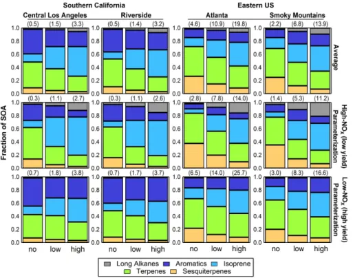
Accounting for vapor wall losses leads to regionally-specific changes in the simulated contributions from the different VOC classes (e.g. TRP1, ARO1) to the SOA burden, as illustrated in Fig. 4 for two sites in SoCAB (central Los Angeles and Riverside) and two in the eastern US (Atlanta and the Smoky Mountains). Focusing first on contribu-tions from the biogenic VOCs, at all locacontribu-tions accounting for vapor wall losses leads to

10

an increase in the fractional contribution of isoprene SOA, typically at the expense of terpene and sesquiterpene SOA. This is true for both the low- and high-NO_x simula-tions. Recent observations suggest that isoprene SOA produced via the low-NO IEPOX (isoprene epoxydiol) pathway can be uniquely identified from analysis of aerosol mass spectrometer measurements when the relative contribution is sufficiently large (&5 %)

15

(e.g. Budisulistiorini et al., 2013; Hu et al., 2015). This observed IEPOX SOA accounts for around 30 % (May) and 40 % (August) of total SOA or around 20 % (May) and 30 % (August) of total OA in Atlanta in the summer (Xu et al., 2015a), albeit not during the same time period as simulated here. IEPOX SOA was also found to account for 17 % of total OA at a rural site in Alabama in 2013 (Hu et al., 2015). The SOM-low and

20

SOM-high simulation results for Atlanta are most consistent with the observations, with a predicted isoprene SOA fraction of 27 and 35 %, respectively, compared to only 17 % for the SOM-no simulations and where the reported values are for the simulations that use the low-NO_xparameterizations since this is the pathway that leads to IEPOX SOA. The related isoprene OA fractions are 10, 21 and 31 % for the SOM-no, -low and -high

25

(21)

ACPD

15, 30081–30126, 2015

C. D. Cappa et al.

Title Page

Tables Figures

◭ ◮

Back Close

Full Screen / Esc

Discussion

P

a

per

|

Discussion

P

a

per

|

Discussion

P

a

per

|

Discussion

P

a

per

|

to 25 and 37 %, respectively. The SOM-no simulations exhibit somewhat greater sensi-tivity to the NO_x parameterization, with the high-NO_x parameterization giving an SOA fraction of 7 %.)

In SoCAB, the predicted average isoprene SOA fraction in central LA is relatively large for the low (36 %) and high (47 %) simulations, compared to the

SOM-5

no simulations (12 %). There is a large difference in SoCAB between the simulations that use the low-NO_x and high-NO_x parameterizations, with the isoprene SOA frac-tions being much larger with the high-NO_x parameterizations (e.g. 58 % for high-NO_x vs. 36 % for low-NO_x for the SOM-high simulations). Measurements at Pasadena dur-ing the 2010 CalNex study did not distinctly identify IEPOX SOA, which is interpreted

10

as the IEPOX SOA contribution being lower than∼5 % of the OA (Hu et al., 2015). It is

possible that additional isoprene SOA had been formed under higher NO_x conditions (compared to the southeast US) such that it is chemically different from IEPOX-SOA and was not identified as a uniquely isoprene-derived SOA component, instead con-tributing generically to the overall oxygenated OA pool. The concentration of isoprene

15

SOA from specific high-NO_xpathways may, however, be limited at higher temperatures, such as found in summertime Pasadena, due to thermal decomposition of intermediate gas-phase species (Worton et al., 2013), although it is not clear to what extent this in-fluenced the CalNex observations or would have affected the model results had it been explicitly considered. Thus, although the CalNex measurements do not provide direct

20

support for such a large isoprene SOA fraction, they also do not rule it out.

While the predicted isoprene SOA fraction increased, the predicted terpene and sesquiterpene SOA fractions decreased in the simulations that accounted for vapor wall losses. Additionally, the terpene SOA/sesquiterpene SOA ratio increased at all loca-tions for the SOM-low and SOM-high simulaloca-tions, in large part because the

sesquiter-25

pene yield is already large and thus accounting for vapor wall losses has a limited influence on the simulated sesquiterpene SOA concentrations.

(22)

an-ACPD

15, 30081–30126, 2015

C. D. Cappa et al.

Title Page

Tables Figures

◭ ◮

Back Close

Full Screen / Esc

Discussion

P

a

per

|

Discussion

P

a

per

|

Discussion

P

a

per

|

Discussion

P

a

per

|

thropogenic fraction is equivalent to the fossil fraction of SOA (termedFSOA,fossil). At the

two eastern US sites (Atlanta and Smokey Mountains) the averageF_SOA,fossilincreases slightly from 14 % (SOM-no) to 22 % (SOM-low) and 25 % (SOM-high). At the two So-CAB sites (downtown LA and Riverside) the predicted average FSOA,fossil decreases

slightly, from 35 % (SOM-no) to 29 % (SOM-low) and 30 % (SOM-high), respectively.

5

In SoCAB the F_SOA,fossil values differ between the low- and high-NO_x parameteriza-tions, with F_SOA,fossil typically larger for the low-NO_x parameterizations (e.g. 35 % for low-NO_x and 25 % for high-NO_x). In the eastern US, the predicted F_SOA,fossil exhibit a stronger response to vapor wall losses for the high-NO_x parameterization than the low-NO_xparameterization, although the absolute values are reasonably similar. Of the

10

anthropogenic SOA (aromatics ₊ alkanes), the high-NO_x parameterizations indicate an increasing alkane SOA fraction as vapor wall losses are accounted for in both re-gions. In contrast, the low-NO_x parameterizations indicate minor contributions from alkane SOA for all of the simulations. In general, chamber SOA yields from aromatic compounds are larger for low-NO_x conditions (Ng et al., 2007a), which could help to

15

explain these differences.

The SoCABF_SOA,fossil values can be compared with estimates of the fossil fraction of “oxidized organic carbon” (F_OOC,fossil) from measurements made during CalNex in Pasadena (Zotter et al., 2014). It should be noted that while F_SOA,fossil includes con-tributions from both oxygen and carbon mass, theF_OOC,fossil includes only the carbon

20

mass. Thus, if there are di_fferences in the O : C atomic ratio between fossil and non-fossil SOA thenF_SOA,fossilandF_OOC,fossilmay not be directly comparable. TheF_OOC,fossil

values were determined from14C analysis of particles collected on filters to allow deter-mination of the fossil fraction of the total carbonaceous material coupled with positive matrix factorization to allow separation of the contributions from the various fossil and

25

non-fossil POA and SOA sources. The uncertainty in the fossil fraction of total OC was reported as 9 %; the uncertainty in theFOOC,fossilwill be larger. Zotter et al. (2014)

(23)

av-ACPD

15, 30081–30126, 2015

C. D. Cappa et al.

Title Page

Tables Figures

◭ ◮

Back Close

Full Screen / Esc

Discussion

P

a

per

|

Discussion

P

a

per

|

Discussion

P

a

per

|

Discussion

P

a

per

|

erage predicted FSOA,fossil (e.g. 30 % for SOM-high). The difference between the

ob-served F_OOC,fossil and predicted F_SOA,fossil could indicate a role for SOA formed from fossil-derived S/IVOC species in the atmosphere, which are not considered here.

3.3.2 The oxygen-to-carbon ratio

The O : C atomic ratios of the SOA have been calculated from the simulated

distribu-5

tions of compounds inN_CandN_Ospace; the O : C atomic ratio is an inherent property of the SOM model and (O : C)_SOAvalues from box model simulations using SOM exhibit generally good agreement with observations (Cappa and Wilson, 2012; Cappa et al., 2013). Few air quality models attempt to simulate O : C ratios for SOA (e.g. Murphy et al., 2011), although a dramatic expansion in observations of O : C ratios for

ambi-10

ent OA has recently occurred (Ng et al., 2011; Canagaratna et al., 2015; Chen et al., 2015). Comparison between intensive properties such as O : C, in addition to absolute OA concentrations, can provide further constraints on the transformation processes and OA sources in a given region. The simulated (O : C)_SOAin the SOM-no simulations are generally larger in SoCAB than in the eastern US (Fig. 6). The simulated (O : C)_SOA

15

from isoprene and aromatics individually are larger than those from mono- or sesquiter-penes due, in large part, to the smaller carbon backbone and the need to add more oxygens to produce su_fficiently low volatility species that partition substantially to the particle phase (Chhabra et al., 2011b; Cappa and Wilson, 2012; Tkacik et al., 2012). Thus, the larger (O : C)_SOAin SoCAB results from larger relative contributions from

iso-20

prene and aromatic compounds to the total SOA burden in this region. The (O : C)_SOA is also generally larger in regions where SOA concentrations are smaller. This may reflect some relationship between SOA source and concentration, but it also reflects the role that continued multi-generational oxidation has on the SOA composition, since lower concentrations can reflect greater dilution and overall more aged SOA.

25

(24)

ACPD

15, 30081–30126, 2015

C. D. Cappa et al.

Title Page

Tables Figures

◭ ◮

Back Close

Full Screen / Esc

Discussion

P

a

per

|

Discussion

P

a

per

|

Discussion

P

a

per

|

Discussion

P

a

per

|

simulated SOA burden in the SOM-low and SOM-high simulations and (ii) differences in the SOM chemical pathways (i.e. the SOM parameters) that lead to the production of condensed-phase material between the parameterizations that do/do not include vapor wall losses. The influence of the latter has been confirmed through box model simula-tions, although the exact behavior is both precursor specific and somewhat dependent

5

on the reaction conditions (e.g. [OH] and the initial precursor concentration). Overall, the former effect likely dominates since the difference in simulated (O : C)_SOA between isoprene and monoterpenes is substantial (Jathar et al., 2015a).

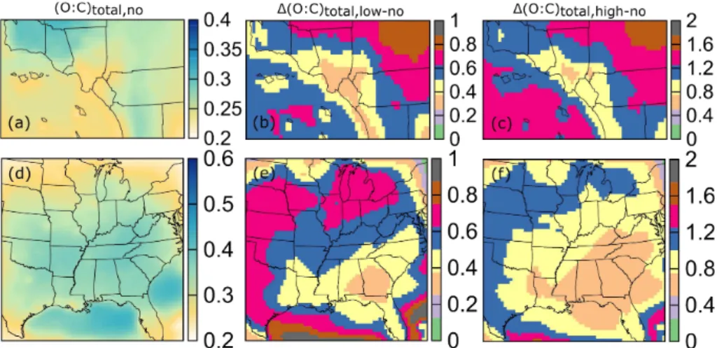
The simulated O : C for the total OA also differs substantially between simulations (Fig. 7), especially in regions where the simulated increase inf_SOA is largest (Fig. 2).

10

The simulated (O : C)_total in both the SoCAB and eastern US increases substantially when vapor wall losses are accounted for. For example, the simulated (O : C)_total val-ues at Riverside were 0.22, 0.3 and 0.42 and at Atlanta were 0.45, 0.65 and 0.85 for SOM-no, SOM-low and SOM-high simulations, respectively. The increase in (O : C)_total is mostly driven by an associated increase inf_SOA. The (O : C)_total value is a weighted

15

average of the (O : C)_SOA and (O : C)_POA, with (O : C)_total=(n_O,SOA+n_O,POA)/(n_C,SOA+

n_C,POA) wheren_O and n_C indicate the number of oxygen and carbon atoms,

respec-tively, that comprise all SOA types and POA. For conceptual purposes, this exact expression for (O : C)_total can be approximated as (O : C)_total∼f_SOA(O : C)_SOA+(1−

f_SOA)(O : C)_POA, where (O : C)_SOArepresents the average over the di_fferent SOA types.

20

Thus, changes in f_SOA lead to changes in (O : C)_total, with some additional smaller changes due to variation in the weighted average (O : C)_SOA between the various sim-ulations (since each SOA type has a particular O : C range). The predicted eastern US (O : C)_totalare generally larger than in SoCAB due to the largerf_SOAin the eastern US and since (O : C)_SOA is typically larger than (O : C)_POA. For example, the average

25

(O : C)_totalin Atlanta for the SOM-no simulations was 0.4 whereas it was 0.22 in River-side.

(25)

reso-ACPD

15, 30081–30126, 2015

C. D. Cappa et al.

Title Page

Tables Figures

◭ ◮

Back Close

Full Screen / Esc

Discussion

P

a

per

|

Discussion

P

a

per

|

Discussion

P

a

per

|

Discussion

P

a

per

|

lution time-of-flight aerosol mass spectrometer (HR-AMS), which determines (O : C)_total with an absolute uncertainty of ±30 % but with very high precision (Docherty et al.,

2008; Dzepina et al., 2009). Values reported here have been corrected according to Canagaratna et al. (2015). The campaign-average observed (O : C)_total was ∼0.45.

The SOM-high (O : C)_total is in very good agreement with the observations, whereas

5

(O : C)_total is too small for both SOM-no and SOM-low. This good correspondence is, of course, sensitive to the assumed (O : C)_POA, here 0.2 based on (Ng et al., 2011). If a smaller (O : C)_POA had been assumed, then either a greater amount of SOA would be required or the simulated (O : C)_SOA would need to be larger to match the SOAR measurements. Docherty et al. (2011) determined there were three POA types during

10

SOAR, with a weighted-average corrected O : C₌0.095, suggesting that the assumed 0.2 is too large. In contrast, Hayes et al. (2013) determined a weighted-average cor-rected O : C=0.25 for the three POA types identified at Pasadena during CalNex. It has been suggested that at least some of the di_fference in the (O : C)_POA between SOAR and CalNex results from greater heterogeneous ageing of the Pasadena POA.

Regard-15

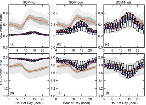
less of the exact (O : C)_POA, a strong improvement in the model-measurement agree-ment when vapor wall losses are accounted for is evident. Of additional consideration is the diurnal dependence of the (O : C)_total. The observed (O : C)_totalexhibited a distinct diurnal dependence, with low values at night, a minimum at∼7 a.m. and maximum

val-ues around midday (Fig. 8). The simulated (O : C)_total diurnal profile for the SOM-high

20

simulations agrees reasonably well with the SOAR observations in terms of both the magnitude of the day-night difference and the absolute (O : C)_total (Fig. 8). In contrast, both the SOM-no and SOM-low exhibit only minor variations with time-of-day due to the controlling influence of (O : C)_POA.

The simulated (O : C)_total values in the eastern US can also be compared with

re-25

(26)

ACPD

15, 30081–30126, 2015

C. D. Cappa et al.

Title Page

Tables Figures

◭ ◮

Back Close

Full Screen / Esc

Discussion

P

a

per

|

Discussion

P

a

per

|

Discussion

P

a

per

|

Discussion

P

a

per

|

0.7, although it should be noted that these values were estimated from measurements made using an Aerodyne aerosol chemical speciation monitor, which increases the uncertainty (Xu et al., 2015b). Measurements made around the southeast US using an HR-AMS onboard the NASA DC8 as part of the SEAC4RS field study indicate the average (O : C)_total₌0.8 when the plane was flying below 1 km (SEAC4RS, 2014). As

5

noted above, the simulated (O : C)_total around Atlanta was 0.45 for SOM-no, increas-ing to∼0.65 for SOM-low and∼0.85 for SOM-high. As with the SoCAB comparison,

the general level of agreement between the observed and simulated (O : C)_tot was im-proved when vapor wall losses were accounted for.

The above simulations included SOA only from VOCs, neglecting contributions from

10

S/IVOCs including oxidation of semi-volatile POA vapors. S/IVOCs and semi-volatile POA vapors are likely ≥C₁₄ carbon species (Jathar et al., 2014; Zhao et al., 2014). As such, little added oxygen is required to produce low-volatility species that will form SOA. Since these species also have relatively large number of carbon atoms, the O : C of the SOA formed from them will be relatively small, most likely with (O : C)_S/IVOC<0.2

15

in the absence of strong heterogeneous oxidation (Cappa and Wilson, 2012; Tkacik et al., 2012); note that this range is lower than what was assumed for the non-volatile POA here. Consequently, had S/IVOCs been included in the simulations the (O : C)_total would have likely decreased. The magnitude of the decrease would depend on the ex-act extent to which the S/IVOCs contributed to the overall SOA burden, the extent to

20

which the simulated POA decreased (due to the semi-volatile treatment), and on the simulated (O : C)_S/IVOC. In the limit that SOA from S/IVOCs dominates the SOA budget, very little variation in the (O : C)_total ratio with time of day would have likely been pre-dicted because (O : C)_POA∼(O : C)_S/IVOC. Additionally, the simulated daytime (O : C)_total

values would have likely been close to 0.2. A lack of diurnal variability and a small

25