Abstract— This work shows the utilization of a coaxial cable for the
fabrication of a long period Bragg grating. The grating is fabricated removing the dielectric in short pieces of the cable so that the discontinuities account for the variation in the medium refractive index. Simulated and experimental results of the grating resonances are shown as a function of the scattering parameters S, demonstrating the feasibility of the technique. By using the sensor in the MHz frequency range cheaper electronics can be employed, which reduce the overall cost of the sensing system.
Index Terms— Long Period Gratings; Coaxial Transmission Lines; Bragg Gratings; Optical Fiber.
I. INTRODUCTION
Transmission lines, by definition, are guided systems used to transmit data and energy in the electromagnetic form [1]. The energy propagates in a longitudinal way, with two or more conductors immersed in a homogenous dielectric connecting a source to a load. For low power applications, transmission lines are used to transmit data in telecommunication systems, whereas they are also used to transport energy in high voltage systems [2-3]. Examples of transmission lines are lines with two parallel or tracing conductors, planar lines or parallel plates, a parallel wire connected to a conductor plane, microstrip lines, optical fiber, and a coaxial cable [4].
Some of these lines are used as sensors for detecting physical quantities such as temperature and strain. For instance, optical fibers have been used with great advantages for this purpose due to its low cost, low signal attenuation and electromagnetic immunity [5-6]. However, they present disadvantages such as the mechanical fragility to transverse stresses and the high cost of the required electro-optical equipment. Although coaxial cables show higher attenuation, they turn out to be more resistant and, depending on the frequency range, they also offer good insulation to electromagnetic interference. At the same time, interrogators and lower cost electronic circuits are available, eliminating the need for expensive electro-optical conversion and contributing to the construction of low-cost sensing systems [7]. Different devices and techniques commonly used in optics for sensing applications, such as Bragg Gratings [8] and Fabry-Perot interferometers [9], have been replicated at lower frequencies in coaxial cables.
Long Period Bragg Grating in Coaxial
Transmission Lines
Sergio Luiz Stevan Jr.1, José Jair Alves Mendes Júnior 1, Frederich Conrad Janzen 1, Murilo Leme Oliveira 1, 1Universidade Tecnológica Federal do Paraná – UTFPR - Ponta Grossa, Brazil,
[email protected],[email protected],[email protected], [email protected], Alexandre de Almeida Prado Pohl 2
2Universidade Tecnológica Federal do Paraná – UTFPR - Curitiba, Brazil,
With this in mind, this work reports on the fabrication and characterization of Long Period Bragg Gratings (LPBG) in coaxial cables, which employ the same concepts of gratings written in optical fibers. Thus, the implementation of Long Period Bragg Gratings in coaxial transmission lines is proposed and described through a mathematical model, simulation and experimental results, demonstrating that they can be used as an option for applications in which gratings fabricated in optical fibers present limitations.
II. COAXIAL TRANSMISSION LINES
A coaxial cable is a transmission line made of a central conductor and a concentric cylindrical ground loop, separated by a dielectric material and extruded to an external polymer-based protection cap [10]. One of the main parameters of coaxial cables is the characteristic impedance, which for commercial cables presents values of either 50 Ω or 75 Ω. The 50 Ω-cable is commonly used for data transmission, while 75 Ω-cables are used in antenna reception systems and broadband networks for transporting digital and analog TV signals [10].
The electric equivalent of the coaxial transmission line of an infinitesimal length Δz is represented by the circuit shown in Figure 1, in which the parameters L, R, C, and G represent its Inductance (H/m), Resistance (Ω/m), Capacitance (F/m), and Conductance (S/m).
LΔz RΔz
CΔz GΔz i(z,t) i(z+Δz,t)
v(z,t) v(z+Δz,t)
Fig. 1: Electric equivalent model of the coaxial transmission line.
Applying Kirchhoff Laws to the circuit shown in Figure 1, one can assess the electric voltage, v(t, z) and the current, i(t, z), along the coaxial line in the time domain. The resulting equations that describe the behavior of v(t, z) and i(t, z) are shown in (1) and (2) [11]
-
dv t,zdt
=R i t,z +L
Δ
z
di t,zdt
,
(1)-
di t,zdt
=G v t,z +C
dv t,zdt
.
(2)Z=
R+jωLG+jωC
.
(3)Solving equations (1) and (2) by means of phasor terms one obtains equations (4) and (5), which refer to the voltage and current in the transmission line along the distance z of the line [11].
d²v(z)
dz²
=
γ
²v(z) ,
(4)d²i(z)
dz²
=
γ
²i(z) .
(5)In such equations γ is the complex propagation constant of the line, given as
γ
=
(R+j
ω
L).(G+j
ω
C)
≡
α
+
j
β
.
(6)The relationship between the cable parameters and the frequency of the signal to be transmitted can also be described by the real part α of (6), which is the attenuation constant given in neper/ meter, and by the imaginary part β, which represents the phase constant in radians/meter. Solving the system of coupled equations given in (4) and (5) one obtains [11]
V(z)=V
0+e
-γz+
V
0-e
γz (7)I(z)=
(V0 +e-γz+ V0-eγz)
Z
=I
0+
e
-γz+ I
0-e
γz,
(8)in such equations V0+ and I0+ represent the amplitude of the signal wave propagating in the positive
direction of z (transmission wave) and V0- e I0- represent the amplitude of the signal wave propagating
in the negative direction of z (reflected wave), respectively.
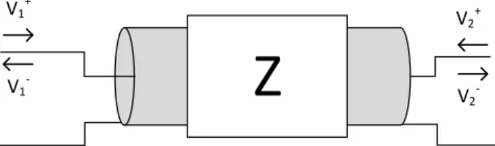
Another method of analyzing the transmission line considers the input and output behavior of the signals in a short path of coaxial cable, along which the fractions of reflected and transmission waves are taken into account. This technique is known in the literature as the Scattering Matrix approach [13-14]. In this case, the path of cable can be represented as a quadrupole (see Figure 2) and the relationship between the input and output signal waves is obtained by the product of matrices, given in (9)
V
1-V
2-=
S
11S
12S
21S
22V
1+Z
V1+
V1
-V2+
V2
-Fig. 2: Coaxial Transmission Line represented by a quadrupole
The Sij coefficients in the 2x2 matrix in (9) are called the Scattering Matrix or simply Scattering
Parameters. S11 and S22 represent the reflection coefficients (Γ), as they quantify how much of one
signal is reflected on either side of the cable patch based on the incident voltage amplitude. On the other hand, the Scattering Parameters S12 e S21 are the transmission coefficients (T), which represent
how much of the input signal on one side is transmitted to the other side. For instance, coefficients S11
and S21 are determined by
Γ
=S
11=
V1-S12V2+ V1+
,
(10)T=S
21=
V2-S22V2+ V1+
,
(11)respectively, in which V1- is the voltage amplitude that is reflected on the left side of the cable patch
seen in Figure 2 and V1+ is the voltage amplitude on the input to the left side. Similarly, V2- represent
the value of the voltage reflected on the right side of the patch and V2+ is the value of voltage
impinging on the right side. Thus, S11 and S21 are the main parameters used to assess the behavior of
the reflected and transmitted waves, respectively, propagating in the transmission line.
III. BRAGG GRATING AND LONG PERIOD BRAGG GRATING
Fig. 3: Interaction of an optical signal band with the Bragg Grating [15]
The fact that the optical properties of gratings are affected by temperature variations and/or mechanical deformations makes them an important and useful sensor [20, 21], which can be applied in different areas, such as biomechanics [22], civil engineering, [23] and aeronautics [24, 25]. The same working principle of gratings, when used in coax cables, presents many advantages, mainly when the final application is devoted to the continuous monitoring of buildings, bridges and other civil engineering constructions.
The behavior of Bragg gratings in optical fibers are described by the Maxwell system of differential equations [11]. In this way, a parallel can be traced between the optical fiber and the coaxial cable, as the signal propagating in them are both governed by the same laws. For instance, when an electromagnetic wave traverses an interface between two different materials, part of it is transmitted and the other is reflected back. The reflectivity accounts for the part that is reflected and is given as
R
F=
(n1-n2)2
(n1+n2)2
,
(12)in which n1 is the refractive index of the incidence medium and n2 is the refractive index of the
transmission medium, respectively. When the discontinuity of the refractive index between the two media is small (n2 ≈n1 - Δn) the reflectivity can be written as
R
F=
n
1- n
1-
Δ
n
n
1+ n
1-
Δ
n
2
=
Δ
n
2
-
Δ
n
2(13)
sum of the reflected power is concentrated in a small band of specific wavelengths, whose maximum value is given by the Bragg relationship
λ
B=2n
effΛ
(14)in which λB is the peak wavelength of the reflection band, neff is the effective index of the propagating
mode in the fiber, and Λ is the spatial period of the refractive index discontinuity. Therefore, these two parameters (effective refractive index and period) have paramount importance on the employment of the Bragg grating in optical fibers and coaxial cables.
Still, the grating behavior [18] can also be explained using the Bragg condition for two interacting modes in the fiber, which propagate in opposite directions, given as
Δβ=β
+-
β
-= 2β= 2π Λ
⁄
.
(15)In (15) β is the propagation constant of a guided mode, the same parameter that appears in (6); β+
and β- represent the constants of the forward propagating and the backward propagating modes,
respectively; Λ is the period of the refractive index discontinuity that characterizes the Bragg grating and Δβ is the difference of the propagation constants involved in the mode coupling. Since the propagation constants are a function of the wavelength, the corresponding phase is highly selective to it [18].
The propagation constant of the fundamental forward propagating mode is given as
β
01=
2πneff,
(16)in which β01 is the fundamental forward constant, λ is the wavelength and
n
effis the effective
refractive index of that mode
. For the reverse (backward) propagating mode, the propagation constant has the same magnitude but opposite sign, as shown in (15). Replacing (15) in (16) one finds the phase matching condition for these two interacting modes given as [18]λ
B=
2neffΛN
,
(17)which leads to the expression in (14) when N = 1. The wavelength λB is the Bragg wavelength in
function of the period of the grating, Λ, and the mode refractive index, neff. In this way, by submitting
the grating to external effects (change of temperature and/or application of strain), both parameters can be changed and the Bragg wavelength will be shifted [26].
These concepts are valid for modes in optical fibers as well as for modes propagating in coaxial cables [27]. The expression
2
β
=
2
π
m
Λ
(18)is similar to (15) and can be used to describe the mode coupling in coaxial cables in which discontinuities are present with m as an integer representing the interaction order [28]. For coaxial cables the propagation constant is evaluated as [29]
β
=2
π
f
√
LC
(19)The expression above describes the propagation constant β, in which f is the frequency related to the propagating mode and L and C are the inductance and capacitance parameters of the coaxial cable. The capacitance can be obtained from the cable datasheet and L can be calculated, for instance, from equation (3) as long as the impedance and attenuation of the coaxial cable are known.
Replacing (19) in (18) gives
2 2
π
f
√
LC =
2mπ Λ∴
f
=
m
2Λ√LC
.
(20)Making vp≡ 1/√LC, in which vp is the phase velocity of the wave in the continuous medium, one obtains =vp/2Λ, for m = 1. That is, the fundamental resonance frequency of the grating structure is directly proportional to the phase velocity and inversely proportional to the grating period. Wei et al [27] derived such equation, which exhibits an efficient form to realize the mode conversion in coaxial cables with periodic discontinuities.
IV. SIMULATION
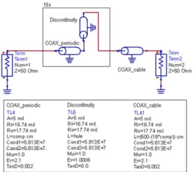
A simulation of the transmission line with discontinuities was performed using the software Agilent Advanced Design System, version 2013.6. Figure 4 shows a schematic diagram of the coaxial transmission line (RG58; 50 Ω) simulated in 5 meters length, in which discontinuities of 2 mm length intercalated along 18 stretches of coaxial cable determine the period Λ of the long period grating. A larger stretch of cable finishes the 5 m length. Simulations with Λ = 7.7 cm, 8.5 cm and 8.7 cm were performed. The discontinuities are represented by the absence of the polyethylene dielectric, and the dielectric constant is set at 1.0006 (air) and the loss tangent is zero. The main parameters of coax cable used in the simulation are: A is the radius of inner conductor; Ri is the inner radius of outer conductor; Ro is the outer radius of outer conductor; L is the length; Cond1 is the plating metal conductivity; Cond2 is the base metal conductivity; Mur is the relative permeability of dielectric; Er is the dielectric constant of the dielectric between the inner and outer conductors; and TanD is the dielectric loss tangent; and the attributed values are presented in figure 4. The parameter comp represents the length between discontinuities and the parameter hole, the length of the discontinuity.
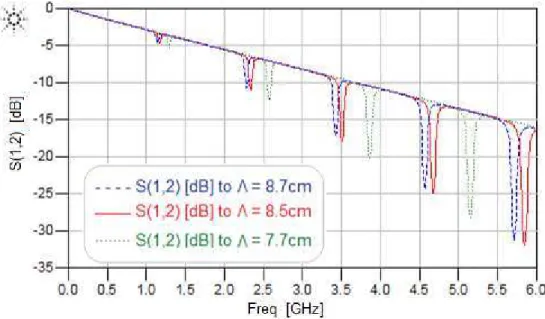
The simulation aims to analyze the propagation of a signal whose frequency varies between 100 MHz to 6 GHz and to observe the transmission and reflection behavior by means of the Scattering Parameters S11 and S12. Figure 5 shows the results of the S12 coefficient for Λ = 7.7 cm (doted curve),
8.5 cm (continuous curve) and 8.7 cm (traced curve), in which an alteration in the discontinuities results in the alteration of the resonance frequency by the grating. One notices that resonances appear at a fundamental frequency and at subsequent harmonics.
Fig. 5: Graphic of parameter S12 by the frequency given by response of the simulations of periods of length of cm and 7.5cm
Considering the distributed parameters L=0.262 µH/m and C=93.5 pF/m for the RG58 cable and using (20), one estimates the phase velocity approximately as 2.02×10⁸ m/s. In this case, the estimated
fundamental resonance frequency is fo=1.141 GHz for Λ=8.7 cm, 1.171 GHz for Λ=8.5 cm and
fo=1.291 GHz for Λ=7.7 cm, respectively. From Figure 5 one notices that the reflection becomes
stronger at higher-order harmonics. However, due to the cable loss, the increase is not linear [30].
V. FABRICATION AND EXPERIMENTAL RESULTS
The LPBG was fabricated removing the dielectric in a stretch of cable so that the discontinuities always have the same width and depth. For this purpose, a circular saw and mold were used, as illustrated in Figure 6. Figures 7a) and 7b) show, respectively, a top and side view of the discontinuity in the cable.
Using a Vector Network Analyzer (VNA), Agilent Model ENA E5071C, set to scan the frequency range between 100 MHz and 3.3 GHz, the parameters S11, S12, S21, and S22 were measured considering
different discontinuity periods in the RG58 (50 Ω) coax cable. Experiments were conducted considering periods of 7.7 cm, 8.7 cm and 25 cm, respectively.
(a) (b)
Fig. 6: Process of making uniform discontinuities Fig. 7: Discontinuities inserted in coaxial cable: a) lateral view; b) upper view.
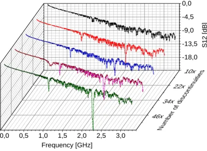
Especially regarding the period Λ=8.7 cm, measurements were conducted for different numbers of discontinuities. Figure 8 shows the evolution of the grating rejection peaks considering the period of 8.7 cm, within the same frequency range, as the number of discontinuities inserted in the cable is increased: 10, 22, 34, 46 and 58, respectively. Thus, one observes that the higher the number of discontinuities, the deeper the resonance amplitude. The portion of the wave matching the reflected part is found as multiple frequencies of 1.141 GHz.
0,0 0,5 1,0 1,5 2,0 2,5 3,0
-18,0 -13,5 -9,0 -4,5 0,0
10x
22x
34x
46x
Frequency [GHz]
S
1
2
[
d
B
]
Num ber
of d isco
ntin uitie
s
Fig. 8: Behavior of parameter S12 as a function of the frequency and the number of discontinuities (grating period Λ=8.7 cm).
Figure 9 shows the comparison between the simulated (continuous line) and experimental (dotted line) values of S12 for the period of 25 cm. One observes that, even if the resonance strength is not
high, multiple frequencies of 400 MHz are seen over the frequency range, whose amplitude are more intense for the higher order harmonics.
VI. CONCLUSION
This paper demonstrates that Long Period Bragg Gratings in coaxial transmission lines can be successfully fabricated, enabling the use of cheaper circuits and sensors. Fabrication of the grating is made possible as changes in the dielectric can be accomplished by removing short pieces of the material along a stretch of cable.
For instance, by fabricating a grating of period 8.7 cm in a RG58 coax type cable, the fundamental 1.141 GHz resonance with 4 dB intensity and resonances deeper than 10 dB for the first harmonic (at 2.281 GHz) have been experimentally observed. It has been also observed that the larger the period of the grating, the lower is the fundamental resonance for sensing purposes. Increasing the number of discontinuities in the stretch of cable also leads to deeper resonance peaks as shown in Figure 8.
Future work on this topic can approach the modeling of discontinuities (such as its number and length) in order to verify their influence on the intensity of the resonance peaks. Moreover, one can improve the design for the sensing element, as the present technique of removing portions of the dielectric is invasive and imposes mechanical variations in the cable structure. Furthermore, one can also investigate the design of cheaper electronic circuits for applications concerning frequencies in the megahertz range, leading to sensing systems that can be implemented as simple and cheap solutions.
REFERENCES
[1] S. M. Wentworth, Eletromagnetismo aplicado: abordagem antecipada das linhas de transmissão, Bookman: São Paulo, 2007, pp. 47-53
[2] G. Miamo, and A. Maffucci, Transmission Lines and Lumped Circuits: Fundamental and Applications. Academic Press: San Diego, California, 2001, pp. 17-21
[3] E. Fontana, “Capítulo 9 Linhas de Transmissão”, Eletromagnetismo – Parte II, Univ. Federal de Pernambuco, http://www.ufpe.br/fontana/ Eletromagnetismo2/EletromagnetismoWebParte02/mag2cap9.htm (current Mar. 25, 2014).
[4] G. S. N. Raju, Electromagnetic field Theory and Transmission Lines. India Pearson Education: Dehli, 2006, pp 414-422.
[5] Hoffmann, Lars, et al. "Applications of fibre optic temperature measurement."Proc. Estonian Acad. Sci. Eng 13.4 (2007): 363-378.
[6] Jin, Long, et al. "An embedded FBG sensor for simultaneous measurement of stress and temperature." Photonics
Technology Letters, IEEE 18.1 (2006): 154-156.
[7] Jie Huang, Tao Wei, Xinwei Lan, Jun Fan and Hai Xiao, “Coaxial cable Bragg grating sensors for large strain measurement with high acuuracy” Proc. SPIE 8345, Sensors and Smart Structures Technologies for Civil, Mechanical, and Aerospace Systems 2012, 83452Z (April, 26, 2012); doi: 10.1117/12.915035.
[8] Huang, Jie, et al. "Coaxial Cable Bragg Grating Sensors for Structural Health Monitoring." International Journal of
Pavement Research and Technology 5.5 (2012): 338-342
[9] Huang J, Wang T, Hua L, Fan J, Xiao H, Luo M. A coaxial cable Fabry-Perot interferometer for sensing applications. Sensors (Basel). 2013, 13, 15252-15260, doi:10.3390/s131115252
[10] E. Salvati and M. A. Ricardo. Estudo de Defeitos em Cabos Coaxiais Através do Método FDTD – Finite Difference Time Domain, monograph, Univ. Federal do Paraná, Curitiba, 2004.R. Nicole, “Title of paper with only first word capitalized,” J. Name Stand. Abbrev., in press.
[11] M. N. O. Sadiku. Elementos de Eletromagnetismo. 5th ed, Bookman, Porto Alegre, 2012, pp.429-481.M. Young, The Technical Writer’s Handbook. Mill Valley, CA: University Science, 1989.
[12] W. H. Hayt Jr. Eletromagnetismo. 3rd. Rio de Janiro: LTC-Livros Técnicos e Científicos Editora Ltda., 1983, pp 329-343.
[13] S. Ramo, J. R. Whinnery, T. V. Duzer. Campos e Ondas em Eletrônica das Comunicações. Guanabara Dois: Rio de Janeiro, 1981, pp 457-461
[14] J.Staples. “Scattering Matrices”. U.S. Particle Accelerator Scholl, http://uspas.fnal.gov/materials/08UCSC/mml14_scattering_matrices.pdf, (current Mar, 31 2014)
[15] L.Y. Shao, J. Zhao, X. Dong, H. Y. Tam, C. Lu, and S. He. “Long Period prating fabricate by periodically tapering standard single-mode fiber”, The Hong Kong Polytechnic University, http://repository.lib.polyu.edu. hk/jspui/bitstream/10397/4331/1/ShaoLong-periodgratingfabricated.pdf. (current Apr. 7, 2014)
[17] S. A. Vasiliev, and O. I. Medvedkov, “Long Period refractive index fiber gratings: properties, applications, and
fabrication techniques” Russian Academy of Sciences,
http:// http://gratings.fo.gpi.ru/pdf/SPIE_2000_4083_212_Vasiliev.pdf (current Apr. 9, 2014)
[18] R. Kashyap, Fiber Bragg Grating. Academic Press: London, 1999.
[19] V. Bhatia, “Properties and Sensing Applications of Long-Period Gratings”, doctoral dissertation, Faculty of the Virginia Polytechnic Institute and State University, Blacksburg, Virginia, 1996.
[20] R. C. S. B. Allil, Sensores a fibra óptica com tecnologia FBG para medida de temperatura e alta tensão, doctoral dissertation, Univ. Federal do Rio de Janeiro. 2010.
[21] S. M. M. Quintero, Aplicações de Sensores a Rede de Bragg em Fibras Ópticas na Medição de pH e Deformação de Filmes Finos de Alta Dureza, máster’s thesis , Pontifícia Univ. Católica do Rio de Janeiro, 2006.
[22] P. Mégret, S. Bette, C. Crunelle, and C. Caucheteur, “Fiber Bragg Gratings: fundamentals and applications”, Univ. de Mons, Electromagnetism & Telecom Department, http://www.telecom.fpms.ac.be/PhotonDoctoralSchool2007/ doc/doct-school07-PMegret-FBG-paper.pdf (current Feb. 23, 2014).
[23] E.Al-Fakih, N. A. A. Osman, F. R. M. Adikan. The use of Fiber Grating sensors in biomechanics and rehabilitation appications: the state-of-the-art and ongoing research topics. Sensors, 2012, pp.12890-12926.
[24] W. L. Schulz, J. P. Conte, E. Udd, J. M. Seim. Static and dynamic testing of bridges and highways using long-gage fiber Bragg grating based strain sensors, Proc. SPIE, Industrial Sensing Systems, Boston, Mass, 2000.
[25] A. Panopoulou, D. Roulias, T. H. Loutas and V. Kostopoulos. “Health monitoring of aerospace structures using Fiber Bragg Gratings Combined with advanced signal processing and pattern recognition techniques”, Strain, Vol. 48, Nº3, June 2012, pp. 267-277.2
[26] James, Stephen W., and Ralph P. Tatam. "Optical fibre long-period grating sensors: characteristics and application." Measurement Science and Technology 14.5 (2003): R49-R61.
[27] T. Wei, S. Wu, J. Huang, H. Xiao, and J. Fan, “Coaxial cable Bragg grating”, Applied Physics Letters, Vol. 99, Issue 11, 2011
[28] Z. Zhou, Y. Li, P. Zhao, and D. Anton, “Novel Coaxial Cable Bragg Grating”, Pacific Science Review, Vol 13, Nº 3, 2011, pp. 196-199
[29] Songping Wu; Tao Wei; Jie Huang; Hai Xiao; Jun Fan, "Modeling of Coaxial Cable Bragg Grating by Coupled Mode Theory," Microwave Theory and Techniques, IEEE Transactions on , vol.62, no.10, pp.2251-2259, Oct. 2014 doi: 10.1109/TMTT.2014.2342672

![Fig. 3: Interaction of an optical signal band with the Bragg Grating [15]](https://thumb-eu.123doks.com/thumbv2/123dok_br/18888033.424302/5.892.275.620.106.348/fig-interaction-optical-signal-band-bragg-grating.webp)