Novel mixed finite element models for nonlinear analysis of
plates
Abstract
In this study, mixed finite element models of plate bend-ing are developed to include other variables (e.g., the mem-brane forces and shear forces) in addition to the general-ized displacements to investigate their effect on nonlinear response. Various finite element models are developed us-ing the weighted-residual statements of suitable equations. The classical plate theory and the first-order shear deforma-tion plate theory are used in this study and the von Karman nonlinear strains are accounted for. Each newly developed model is examined and compared with displacement finite element models to evaluate their performance. Numerical re-sults show that the new mixed models developed herein show better accuracy than existing displacement based models. Keywords
plates, nonlinear analysis, finite elements, mixed nodes, least-squares method.
Wooram Kim+ and J. N. Reddy∗
Advanced Computational Mechanics Labora-tory, Department of Mechanical Engineering, Texas A&M University, College Station, TX 77843-3123 – USA
Received 2 Feb 2010; In revised form 15 Mar 2010
∗Author email: [email protected]
+
currently at Department of Me-chanical Engineering, Korea Army Academy at Yeong cheon, Yeong cheon, 770-849 South Korea
1 INTRODUCTION
The basic idea of mixed finite element model is to treat stresses or stress resultants as dependent unknowns in addition to the generalized displacements. Certain mixed finite element models of plates were developed more than two decades ago by Putcha and Reddy [3, 4] to overcome the drawbacks of the displacement based models. The mixed finite element models [3, 4] were developed in the past by including bending moments as independent variables to reduce the differentiability of the transverse displacement. The mixed models can provide the same level of accuracy for the bending moments as that for the displacements, whereas in the displacement based model the bending moments are calculated at points other than nodes in the post-processing. Thus, the displacement finite element models cannot provide the same level of accuracy for force-like variables as the mixed finite element models.
are used to develop alternative finite element models to the conventional displacement-based finite element models [5, 7, 8].
In the present study, mixed finite element models are developed to include other variables (i.e., the membrane forces and shear forces) in addition to the bending moments, and to see the effect of them on the nonlinear analysis. The effect of including other variables will be compared with different mixed models to show the advantage of the one type of model over other models. Two different mixed models based on the classical plate theory and two mixed models based on the first-order shear deformation plate theory are developed. The performance of the newly developed finite element models is evaluated by comparing the solutions with those of the existing displacement finite element models [9, 10].
2 REVIEW OF PLATE THEORIES
Here we derive governing equations of the classical plate theory (CPT) and first-order shear deformation theory (FSDT) of plates with the von Karman strains. The principle of virtual displacements is used to derive the equilibrium equations in terms of the stress resultants and then the stress resultants are expressed in terms of the displacements using elastic constitutive relations. We only summarize the pertinent equations in this section without presenting the details of the derivation.
The classical plate theory (CPT) is based on the Kirchhoff hypothesis, which consists of the following three assumptions: (1) straight lines perpendicular to the mid-surface (i.e. transverse normals) before deformation, remain straight after deformation; (2) the transverse normals do not experience elongation (i.e. they are in-extensible); (3) the transverse normals rotate such that they remain perpendicular to the mid-surface after deformation. On the other hand, the first-order shear deformation plate theory (FSDT) is based on the assumption the normals before deformation do not remain normal after deformation. Thus, the major difference between the kinematics of the CPT and FSDT is that the normality condition of CPT is relaxed in the FSDT, as illustrated in Fig. 1.
The equations of equilibrium expressed in terms of the stress resultants are the same in both theories, and they are given by
−∂Nxx
∂x − ∂Nxy
∂y =0,
−∂Nxy
∂x − ∂Nyy
∂y =0, ∂
∂x(Nxx ∂w0
∂x +Nxy ∂w0
∂y +Qx)+ ∂ ∂y(Nxy
∂w0
∂x +Nyy ∂w0
∂y +Qy)+q(x)=0, Qx−(
∂Mxx ∂x +
∂Mxy ∂y )=0,
Qy−( ∂Mxy
∂x + ∂Myy
Figure 1 Undeformed and deformed edges in the CPT and FSDT theories (from [10]).
where the stress resultants are defined by
⎧⎪⎪⎪ ⎨⎪⎪⎪ ⎩
Nxx Nyy Nxy
⎫⎪⎪⎪ ⎬⎪⎪⎪ ⎭
=∫ h
2
−h 2
⎧⎪⎪⎪ ⎨⎪⎪⎪ ⎩
σxx σyy σxy
⎫⎪⎪⎪ ⎬⎪⎪⎪ ⎭
dz,
⎧⎪⎪⎪ ⎨⎪⎪⎪ ⎩
Mxx Myy Mxy
⎫⎪⎪⎪ ⎬⎪⎪⎪ ⎭
=∫ h
2
−h 2
⎧⎪⎪⎪ ⎨⎪⎪⎪ ⎩
σxx σyy σxy
⎫⎪⎪⎪ ⎬⎪⎪⎪ ⎭
zdz,
{ Qy Qx }
=∫ h
2
−h 2
{ yz xz }
dz. (2)
Here h denotes the total thickness of the plate and the (x,y)-plane is taken to coincide
with the middle plane of the plate and thez-coordinate is taken perpendicular to the plane of
the plate. The difference in the kinematics of each plate theory is responsible for the difference in the relationships between the stress resultants and the generalized displacements.
2.1 The Classical Plate Theory
u1=u(x, y, z)=u0(x, y)−z(
∂w0(x, y)
∂x ),
u2=v(x, y, z)=v0(x, y)−z(
∂w0(x, y)
∂y ),
u3=w(x, y, z)=w0(x, y). (3)
Under the assumption of small strain but moderately large rotation, we can simplify the components of the nonlinear strain tensor [6, 9, 10]. The components of the Green strain tensor for this case, with the assumed displacement field in (3), are given by
εxx= ∂u0
∂x +
1 2(
∂w0
∂x )
2
−z∂
2w 0
∂x2 ,
εyy= ∂v0
∂y +
1 2(
∂w0
∂y )
2
−z∂
2w 0
∂y2 ,
εxy=
1
2(
∂u0
∂y + ∂v0
∂x + ∂w0
∂x ∂w0
∂y −2z ∂2w
0
∂x∂y). (4)
We assume that the plate is made of linear elastic material and that the plane stress exists. Then the plane stress-reduced elastic constitutive equations are given by
⎧⎪⎪⎪ ⎨⎪⎪⎪ ⎩
σxx σyy σxy
⎫⎪⎪⎪ ⎬⎪⎪⎪ ⎭
=
⎡⎢ ⎢⎢ ⎢⎢ ⎣
Q11 Q12 0
Q12 Q22 0
0 0 Q66
⎤⎥ ⎥⎥ ⎥⎥ ⎦
⎧⎪⎪⎪ ⎨⎪⎪⎪ ⎩
εxx εyy
2εxy
⎫⎪⎪⎪ ⎬⎪⎪⎪ ⎭
, (5)
where the components of the elasticity matrix[Q] are given by
Q11=
E1 1−ν12ν21
, Q12=
ν12E2 1−ν12ν21
= ν21E1
1−ν12ν21
,
Q22= E2
1−ν12ν21
, Q66= G12. (6)
HereE1andE2denote the elastic moduli along the principal material coordinate directions,
which are assumed to coincide with the plate x and y-directions, ν12 and ν21 are Poisson’s
ratios, andG12 is the shear modulus.
Nxx=A11[
∂u0
∂x +
1 2(
∂w0
∂x )
2
]+A12[
∂v0
∂y +
1 2(
∂w0
∂y )
2 ],
Nyy=A12[
∂u0
∂x +
1 2(
∂w0
∂x )
2
]+A22[
∂v0
∂y +
1 2(
∂w0
∂y )
2 ],
Nxy=A66(
∂u0
∂y + ∂v0
∂x + ∂w0
∂x ∂w0
∂y ),
Mxx=−D11(
∂2w0
∂x2 ) −D12(
∂2w0
∂y2 ),
Myy=−D12(
∂2w0
∂x2 )−D22(
∂2w0
∂y2 ),
Mxy=−2D66(
∂2w0
∂x∂y), (7)
where the plate extensional and bending stiffnesses are defined as
(Aij, Dij)=∫ h/2 −h/2
Qij(1, z)dz. (8)
fori, j=1, 2, 6 .
2.2 The First Order Shear Deformation Theory
The displacement field of the FSDT is given by
u1=u(x, y, z)=u0(x, y)+zϕx(x, y), u2=v(x, y, z)=v0(x, y)+zϕy(x, y),
u3=w0(x, y). (9)
The von Karman nonlinear strains of the FSDT are given by
εxx= ∂u0
∂x +
1 2(
∂w0
∂x )
2
+z∂ϕx ∂x ,
εyy= ∂v0
∂y +
1 2(
∂w0
∂y )
2
+z∂ϕy ∂y ,
εxy =
1 2[
∂u0
∂y + ∂v0
∂x + ∂w0
∂x ∂w0
∂y +z( ∂ϕx
∂y + ∂ϕy
∂x )],
εxz= ∂w0
∂x +ϕx, εyz= ∂w0
The plate constitutive equations in the FSDT are given by
Nxx=A11[∂u0 ∂x +
1 2(
∂w0
∂x )
2
]+A12[
∂v0
∂y+
1 2(
∂w0
∂y )
2 ],
Nyy=A12[
∂u0
∂x+
1 2(
∂w0
∂x )
2
]+A22[
∂v0
∂y +
1 2(
∂w0
∂y )
2 ],
Nxy=A66(
∂u0
∂y + ∂v0
∂x + ∂w0
∂x ∂w0
∂y ),
Qx=KsA55(
∂w0
∂x +ϕx) Qy=KsA44(
∂w0
∂y +ϕy) Mxx=D11(
∂ϕx
∂x )+D12( ∂ϕy
∂y ),
Myy=D12(
∂ϕx
∂x )+D22( ∂ϕy
∂y ),
Mxy =D66(∂ϕx ∂y +
∂ϕy
∂x ), (11)
where,Ks(=5/6) is the shear correction factor. We introduce the effective shear forces as
Vx=Qx+(Nxx ∂w0
∂x +Nxy ∂w0
∂y ),
Vy=Qy+(Nxy ∂w0
∂x +Nyy ∂w0
∂y ). (12)
3 FINITE ELEMENT MODELS
3.1 Summary of equations
Governing equations of the CPT
−∂Nxx
∂x − ∂Nxy
∂y =0,
−∂Nxy
∂x − ∂Nyy
∂y =0,
−∂Vx
∂x − ∂Vy
∂y −q(x)=0,
Vx−( ∂Mxx
∂x + ∂Mxy
∂y +Nxx ∂w0
∂x +Nxy ∂w0
∂y )=0,
Vy−( ∂Mxy
∂x + ∂Myy
∂y +Nxy ∂w0
∂x +Nyy ∂w0
∂y )=0, (13)
and
A∗
11Nxx+A
∗
12Nyy=[ ∂u0
∂x +
1 2(
∂w0
∂x )
2 ]
A∗
12Nxx+A
∗
22Nyy=[ ∂v0
∂y +
1 2(
∂w0
∂y )
2 ],
A∗
66Nxy =( ∂u0
∂y + ∂v0
∂x + ∂w0
∂x ∂w0
∂y ),
D∗
11Mxx+D
∗
12Myy=−(∂ 2w
0
∂x2 ),
D∗
12Mxx+D
∗
22Myy=−( ∂2w
0
∂y2 ),
D∗
66Mxy=−2( ∂2w0
∂x∂y). (14)
Governing equations of the FSDT
−∂Nxx
∂x − ∂Nxy
∂y =0,
−∂Nxy
∂x − ∂Nyy
∂y =0, ∂
∂x(Nxx ∂w0
∂x +Nxy ∂w0
∂y +Qx)+ ∂ ∂y(Nxy
∂w0
∂x +Nyy ∂w0
∂y +Qy)+q(x)=0, Qx−(
∂Mxx ∂x +
∂Mxy ∂y )=0,
Qy−( ∂Mxy
∂x + ∂Myy
and
A∗
11Nxx+A
∗
12Nyy=[∂u0 ∂x +
1 2(
∂w0
∂x )
2 ] ,
A∗
12Nxx+A
∗
22Nyy=[ ∂v0
∂y +
1 2(
∂w0
∂y )
2 ],
A∗
66Nxy =(∂u0 ∂y +
∂v0
∂x + ∂w0
∂x ∂w0
∂y ),
0=− Qx
KsA55
+(∂w0
∂x +ϕx),
0=− Qy
KsA44
+(∂w0
∂y +ϕy), D∗
11Mxx+D
∗
12Myy=(
∂ϕx ∂x ),
D∗
12Mxx+D
∗
22Myy=(
∂ϕy ∂y ),
D∗
66Mxy=(
∂ϕx ∂y +
∂ϕy
∂x ). (16)
where A∗
ij and D
∗
ij are inverses of the stiffness matrices: A
∗
=A−1 and D∗=D−1.
3.2 Finite Element Model I (CPT)
In this mixed finite model of the CPT, eleven variables, u0, v0, w0, Nxx, Nyy, Nxy, Vx, Vy,
Mxx, Myy and Mxy, are treated as independent variables. The following weighed-residual
statements are used:
∫Ω
e
(∂W1
∂x N a xx+
∂W1
∂y N a
xy)dxdy−∮
Γe
W1{nxNxx+nyNxy}ds=0,
∫Ω
e
(∂W2
∂x N a xy+
∂W2
∂y N a
yy)dxdy−∮
Γe
W2{nxNxy+nyNyy}ds=0,
∫Ωe(∂W∂x3Vxa+∂W3
∂y V a
y −W3q(x))dxdy−∮ Γe
W3{nxVx+nyVy}ds=0,
∫Ω
e
W4{−A ∗
11Nxxa −A
∗
12Nyya +[ ∂ua
0
∂x +
1 2(
∂wa
0
∂x )
2
]}dxdy=0,
∫Ω
e
W5{−A ∗
12Nxxa −A
∗
22Nyya +[ ∂va0
∂y +
1 2(
∂wa0 ∂y )
2
]}dxdy=0,
∫Ω
e
W6[−A ∗
66Nxya +( ∂ua
0
∂y + ∂va
0
∂x +
1 2
∂wa
0
∂x ∂wa
0
∂y +
1 2
∂wa
0
∂x ∂wa
0
∫Ω
e
W7(−Vxa+
∂Mxxa ∂x +
∂Mxya ∂y +N
a xx
∂wa0 ∂x +Nxy
∂wa0
∂y )dxdy=0,
∫ΩeW8(−Vya+
∂Mxya ∂x +
∂Myya ∂y +N
a xy
∂w0a ∂x +N
a yy
∂wa0
∂y )dxdy=0,
∫Ωe(−D∗
11W9Mxxa −D
∗
12W9Myya + ∂W9
∂x ∂wa0
∂x )dxdy −∮Γe
W9(nx ∂w0
∂x )ds=0,
∫Ω
e
(−D∗
12W10Mxxa −D
∗
22W10Myya + ∂W10
∂y ∂wa
0
∂y )dxdy−∮Γe
W10(ny ∂w0
∂y )ds=0,
∫Ω
e
(−D∗
66W11Mxya +
∂W11
∂x ∂wa0
∂y + ∂W11
∂y ∂wa0
∂x )dxdy
−∮ Γe
W11(nx ∂w0
∂y +ny ∂w0
∂x )ds=0. (17)
where, Γeis the boundary of a typical element region Ωe, variables with a superscript ‘a’ denote
the approximated variables, and nx and ny denote the x and y components (i.e. direction
cosines) of the unit normal vector on the boundary. The primary variables and the secondary variable of the formulation are as follows.
Primary variables Secondary variables
u0 nxNxx+nyNxy v0 nxNxy+nyNyy w0 nxVx+nyVy Mxx nx∂w∂x0 Myy ny∂w∂y0 Mxy nx∂w∂y0+ny∂w∂x0
With the weighted residual statements in (17), we can develop the finite element model, denoted as Model I, of the CPT by approximating the 11 variables with known interpolation functions and unknown nodal values. The Lagrange interpolation functions are admissible for
all variables (i.e.,C0 continuity of all variables is required). We take
u0≅ua0=
m
∑
j=1
ψu0
j (x, y)uj, W1=ψiu0(x, y),
v0≅v0a=
m
∑
j=1
ψv0
j (x, y)vj, W2=ψiv0(x, y),
w0≅w0a=
n
∑
j=1
ψw0
j (x, y)wj, W3=ψiw0(x, y),
Nxx≅Nxxa = p
∑
j=1
ψNxxj (x, y)N1j, W4=ψNxx
Nyy≅Nyya = p
∑
j=1
ψNyyj (x, y)N2j, W5=ψ
Nyy
i (x, y),
Nxy≅Nxya = p
∑
j=1
ψNxyj (x, y)N3j, W6=ψNxy
i (x, y),
Vx≅Vxa= q
∑
j=1
ψjVx(x, y)V1
j, W7=ψiVx(x, y),
Vy≅Vya= q
∑
j=1
ψjVy(x, y)V2j, W8=ψiVy(x, y),
Mxx≅Mxxa = r
∑
j=1
ψMxxj (x, y)M1j, W9=ψMxx
i (x, y),
Myy≅Myya = r
∑
j=1
ψjMyy(x, y)M2j, W10=ψMyyi (x, y),
Mxy≅Mxya = r
∑
j=1
ψjMxy(x, y)M3j, W11=ψMxy
i (x, y). (18)
By substituting the expressions from (18) into the weighted-residual statements of (17), we obtain the finite element equations
⎡⎢ ⎢⎢ ⎢⎢ ⎢⎢ ⎢⎢ ⎢⎣
[K(1)(1)] ⋯ [K(1)( 6)]
⋮ ⋱ ⋮
[K(6)(1)] ⋯ [K(6)( 6)]
⋯ [K( 1)( 11)]
⋰ ⋮
⋯ [K( 6)( 11)]
⋮ ⋰ ⋮
[K(11)(1)] ⋯ [K(11)(6)]
⋱ ⋮
⋯ [K(11)(11)]
⎤⎥ ⎥⎥ ⎥⎥ ⎥⎥ ⎥⎥ ⎥⎦ ⎧⎪⎪⎪⎪ ⎪⎪⎪⎪ ⎨⎪⎪⎪ ⎪⎪⎪⎪⎪ ⎩
{uj}
⋮
{N3j}
⋮
{M3j}
⎫⎪⎪⎪⎪ ⎪⎪⎪⎪ ⎬⎪⎪⎪ ⎪⎪⎪⎪⎪ ⎭ = ⎧⎪⎪⎪⎪ ⎪⎪⎪⎪ ⎨⎪⎪⎪ ⎪⎪⎪⎪⎪ ⎩
{F(1)}
⋮
{F(6)}
⋮
{F(11)}
⎫⎪⎪⎪⎪ ⎪⎪⎪⎪ ⎬⎪⎪⎪ ⎪⎪⎪⎪⎪ ⎭ . (19) where
[K14]=∫
Ωe
{∂ψui0 ∂x ψ
Nxx
j }dxdy, [K
16]= ∫Ω
e
{∂ψui0 ∂y ψ
Nxy
j }dxdy,
[K25]=∫
Ωe
{∂ψvi0 ∂y ψ
Nyy
j }dxdy, [K
26]= ∫Ω
e
{∂ψvi0 ∂x ψ
Nxy
j }dxdy,
[K37]=∫
Ωe
{∂ψwi0 ∂x ψ
Vx
j }dxdy, [K
38]=
∫Ωe{∂ψ
w0
i ∂y ψ
Vy
j }dxdy,
[K41]=∫
Ωe
{ψiNxx∂ψ u0
j
∂x }dxdy, [K
43]
=∫
Ωe
{1
2(
∂w0a
∂x )ψ
Nxx i
∂ψw0
j
∂x }dxdy
[K44]=∫
Ωe
{−A∗ 11ψ
Nxx i ψ
Nxx
j }dxdy, [K
45]=
∫Ωe{−A∗ 12ψ
Nxx i ψ
Nyy
j }dxdy,
[K52]=∫
Ωe
{ψiNyy∂ψ v0
j
∂y }dxdy, [K
53]
=∫
Ωe
{1
2(
∂w0a ∂y )ψ
Nyy i
∂ψw0
j
[K54]=∫
Ωe
{−A∗ 12ψ
Nyy i ψ
Nxx
j }dxdy, [K
55]= ∫Ω
e
{−A∗ 22ψ
Nyy i ψ
Nyy
j }dxdy,
[K61]=∫
Ωe
{ψNxyi ∂ψ u0
j
∂y }dxdy, [K
62]
=∫
Ωe
{ψiNxy∂ψ v0
j
∂x }dxdy,
[K66]=∫
Ωe
{−A∗ 66ψ
Nxy i ψ
Nxy
j }dxdy,
[K63]= ∫Ω
e
{1 2[(
∂wa0 ∂x )ψ
Nxy i
∂ψjw ∂y +(
∂wa0 ∂y )ψ
Nxy i
∂ψjw
∂x ]}dxdy,
[K74]=∫
Ωe
{(∂wa0 ∂x )ψ
Vx i ψ
Nxx
j }dxdy, [K
76]
=∫
Ωe
{(∂wa0 ∂y )ψ
Vx i ψ
Nxy
j }dxdy,
[K77]=∫
Ωe
{−ψiVxψjVx}dxdy, [K79]=∫
Ωe ⎧⎪⎪ ⎨⎪⎪ ⎩ψ Vx i
∂ψjMxx ∂x
⎫⎪⎪ ⎬⎪⎪ ⎭dxdy, [K7(11)]=∫
Ωe ⎧⎪⎪ ⎨⎪⎪ ⎩ψ Vx i
∂ψjMxy ∂y
⎫⎪⎪ ⎬⎪⎪ ⎭dxdy, [K85]=∫
Ωe
{(∂wa0 ∂y )ψ
Vy i ψ
Nyy
j }dxdy, [K
86]
=∫
Ωe
{(∂wa0 ∂x )ψ
Vy i ψ
Nxy
j }dxdy,
[K88]=∫
Ωe
{−ψVyi ψVyj }dxdy, [K8(10)]=∫
Ωe
⎧⎪⎪ ⎨⎪⎪ ⎩
ψiVy∂ψ Myy j ∂y ⎫⎪⎪ ⎬⎪⎪ ⎭ dxdy,
[K8(11)]=∫
Ωe ⎧⎪⎪ ⎨⎪⎪ ⎩ψ Vy i
∂ψjMxy ∂x
⎫⎪⎪ ⎬⎪⎪ ⎭dxdy, [K93]=∫
Ωe
{∂ψiMxx ∂x
∂ψw0
j
∂x }dxdy, [K
99]
=∫
Ωe
{−D∗
11ψiMxxψ Mxx
j }dxdy,
[K9(10)]=∫
Ωe
{−D∗ 12ψ
Mxx i ψ
Myy j }dxdy
[K(10)3]=∫
Ωe
{∂ψMxxi ∂y
∂ψw0
j
∂y }dxdy, [K
(10)9]= ∫Ω
e
{−D∗ 12ψ
Myy i ψ
Mxx
j }dxdy,
[K(10)(10)]=∫
Ωe
{−D∗ 22ψ
Myy i ψ
Myy
j }dxdy,
[K(11)3]= ∫Ω
e
⎧⎪⎪ ⎨⎪⎪ ⎩
∂ψiMxy ∂x
∂ψw0
j ∂y +
∂ψiMxy ∂y
∂ψw0
j ∂x
⎫⎪⎪ ⎬⎪⎪ ⎭dxdy, [K(11)(11)]=∫
Ωe
{−D∗ 66ψ
Mxy i ψ
Mxy
j }dxdy.
{F1}=∮
Γe
ψui {nxNxx+nyNxy}ds , {F2}=∮
Γe
ψiv{nxNxy+nyNyy}ds ,
{F3}=∫
Ωe
{ψiwq(x)}dxdy+∮ Γe
ψwi Qnds {F9}=∮
Γe
ψiMxx(∂w0
{F(10)}=∮
Γe
ψiMyy(∂w0
∂y ny)ds,
{F(11)}=∮
Γe
{ψiMxy(∂w0 ∂y nx+
∂w0
∂x ny)}ds. (20)
The rest of the coefficients matrices and force vectors are zero.
3.3 Finite Element Model II (CPT)
The shear forcesVx andVycan be eliminated by substituting the forth and the fifth equilibrium
equations into the third equilibrium equation of the CPT. The following 9 weighted-residual statements are used:
∫Ωe(∂W∂x1Nxxa +∂W1
∂y N a
xy)dxdy−∮
Γe
W1{nxNxx+nyNxy}ds=0,
∫Ω
e
(∂W2
∂x N a xy+
∂W2
∂y N a
yy)dxdy−∮
Γe
W2{nxNxy+nyNyy}ds=0,
∫Ω
e
{∂W3
∂x ( ∂Mxxa
∂x + ∂Mxya
∂y +N a xx
∂wa0 ∂x +Nxy
∂w0a ∂y )
+∂W3
∂y ( ∂Mxya
∂x + ∂Myya
∂y +N a xy
∂wa0 ∂x +N
a yy
∂wa0
∂y )−W3q(x)}dxdy
−∮ Γe
W3{nxVx+nyVy}ds=0,
∫Ω
e
W4{−A ∗
11Nxxa −A
∗
12Nyya +[ ∂ua
0
∂x +
1 2(
∂wa
0
∂x )
2
]}dxdy=0
∫Ω
e
W5{−A ∗
12Nxxa −A
∗
22Nyya +[ ∂va0
∂y +
1 2(
∂wa0 ∂y )
2
]}dxdy=0,
∫Ω
e
W6[−A ∗
66Nxya +( ∂ua
0
∂y + ∂va
0
∂x +
1 2
∂wa
0
∂x ∂wa
0
∂y +
1 2
∂wa
0
∂x ∂wa
0
∂y )]dxdy=0,
∫Ω
e
(−D∗
11W7Mxxa −D ∗
12W7Myya +
∂W7
∂x ∂wa0
∂x )dxdy−∮Γe
W7(nx ∂w0
∂x )ds=0,
∫Ωe(−D∗
12W8Mxxa −D
∗
22W8Myya + ∂W8
∂y ∂wa0
∂y )dxdy−∮Γe
W8(ny ∂w0
∂y )ds=0,
∫Ωe(−D∗
66W9Mxya + ∂W9
∂x ∂wa0
∂y + ∂W9
∂y ∂wa0
∂x )dxdy−∮Γe
W9(nx ∂w0
∂y +ny ∂w0
∂x )ds=0, (21)
⎡⎢ ⎢⎢ ⎢⎢ ⎢⎢ ⎢⎢ ⎢⎣
[K(11)] ⋯ [K(14)]
⋮ ⋱ ⋮
[K(41)] ⋯ [K(44)]
⋯ [K(19)]
⋰ ⋮
⋯ [K(69)]
⋮ ⋰ ⋮
[K(91)] ⋯ [K(96)]
⋱ ⋮
⋯ [K(99)]
⎤⎥ ⎥⎥ ⎥⎥ ⎥⎥ ⎥⎥ ⎥⎦ ⎧⎪⎪⎪⎪ ⎪⎪⎪⎪ ⎨⎪⎪⎪ ⎪⎪⎪⎪⎪ ⎩
{uj} ⋮
{N1
j} ⋮
{M3
j} ⎫⎪⎪⎪⎪ ⎪⎪⎪⎪ ⎬⎪⎪⎪ ⎪⎪⎪⎪⎪ ⎭ = ⎧⎪⎪⎪⎪ ⎪⎪⎪⎪ ⎨⎪⎪⎪ ⎪⎪⎪⎪⎪ ⎩
{F(1)}
⋮
{F(4)}
⋮
{F(9)}
⎫⎪⎪⎪⎪ ⎪⎪⎪⎪ ⎬⎪⎪⎪ ⎪⎪⎪⎪⎪ ⎭ . (22)
where the coefficients can be easily identified from the weighted-residual statements in (20).
3.4 Finite Element Model III (FSDT)
Model III is based on the following 13 weighed-residual statements of the FSDT:
∫Ω
e
(∂W1
∂x N a xx+ ∂W1 ∂y N a
xy)dxdy−∮
Γe
W1(nxNxx+nyNxy)ds=0,
∫Ωe(∂W∂x2Nxya +∂W2
∂y N a
yy)dxdy−∮
Γe
W2(nxNxy+nyNyy)ds=0,
∫Ω
e
[∂W3
∂x Q a x + ∂W3 ∂y Q a y+ ∂W3
∂x (N a xx
∂wa
0
∂x +N a xy
∂wa
0
∂y )+ ∂W3
∂y (N a xy
∂wa
0
∂x +N a yy
∂wa
0
∂y )
−W3q(x)]dxdy
+∮ Γe
W3[(Qx+Nxx ∂w0
∂x +Nxy ∂w0
∂y )nx+(Qy+Nxy ∂w0
∂x +Nyy ∂w0
∂y )ny]ds=0,
∫Ωe(∂W∂x4Mxxa +∂W4
∂y M a
xy+W4Qax)dxdy+∮
Γe
W4(Mxxnx+Mxyny)ds=0,
∫Ω
e
(∂W5
∂x M a xy+ ∂W5 ∂y M a
yy+W5Qay)dxdy+∮ Γe
W5(Mxynx+Myyny)ds=0,
∫Ω
e
W6{−A ∗
11Nxxa −A
∗
12Nyya +[ ∂ua0
∂x +
1 2(
∂w0a ∂x )
2
]}dxdy=0,
∫ΩeW7{−A ∗ 12N
a xx−A
∗ 22N
a yy+[
∂va0 ∂y +
1 2(
∂wa0 ∂y )
2
]}dxdy=0,
∫Ω
e
W8[−A ∗
66Nxya +( ∂ua0
∂y + ∂v0a
∂x +
1 2
∂w0a ∂x
∂w0a ∂y +
1 2
∂wa0 ∂x
∂w0a
∂y )]dxdy=0,
∫Ω
e W9(−
Qa x KsA55
+∂w
a
0
∂x +ϕ a
∫Ω
e
W10(−
Qay KsA44
+∂w
a
0
∂y +ϕ a
y)dxdy=0,
∫Ω
e
W11(−D ∗
11Mxxa −D
∗ 12Myya +
partialϕa x
∂x )dxdy=0,
∫ΩeW12(−D ∗
12M
a xx−D
∗
22M
a yy+
partialϕay
∂y )dxdy=0,
∫ΩeW13(−D ∗ 66Mxya +
∂ϕax ∂y +
∂ϕay
∂x )dxdy=0. (23)
where Ωe and Γe denote the element region and its boundary, respectively. The primary
variables and the secondary variable of the Model III can be specified as follows:
Primary variable Secondary variable
u0 nxNxx+nyNxy v0 nxNxy+nyNyy w0 Vxnx+Vyny ϕx Mxxnx+Mxyny ϕy Mxynx+Myyny
The finite element model is of the form
⎡⎢ ⎢⎢ ⎢⎢ ⎢⎢ ⎢⎢ ⎢⎣
[K(1)(1)] ⋯ [K( 1)( 7)]
⋮ ⋱ ⋮
[K(7)(1)] ⋯
⋯ [K(1)( 13)]
⋰ ⋮
⋯ [K(7)( 13)]
⋮ ⋰ ⋮
[K(13)(1)] ⋯ [K(13)(6)]
⋱ ⋮
⋯ [K(13)(13)]
⎤⎥ ⎥⎥ ⎥⎥ ⎥⎥ ⎥⎥ ⎥⎦
⎧⎪⎪⎪⎪ ⎪⎪⎪⎪ ⎨⎪⎪⎪ ⎪⎪⎪⎪⎪ ⎩
{uj} ⋮
{N2
j} ⋮
{M3
j} ⎫⎪⎪⎪⎪ ⎪⎪⎪⎪ ⎬⎪⎪⎪ ⎪⎪⎪⎪⎪ ⎭
=
⎧⎪⎪⎪⎪ ⎪⎪⎪⎪ ⎨⎪⎪⎪ ⎪⎪⎪⎪⎪ ⎩
{F(1)}
⋮
{F(7)}
⋮
{F(13)}
⎫⎪⎪⎪⎪ ⎪⎪⎪⎪ ⎬⎪⎪⎪ ⎪⎪⎪⎪⎪ ⎭
. (24)
The coefficients can be identified with the help of the weighted-residual statements in (23).
3.5 Finite Element Model IV (FSDT)
The in-plane forces (Nxx, Nxyand Nyy) can be eliminated by substituting from the first two
equilibrium equations into the remaining equations of equilibrium. The weighted-residual statements of the resulting 10 equations are summarized below:
∫Ω
e
{∂W1
∂x [A11( ∂ua0
∂x +
1 2(
∂wa0 ∂x )
2
)+A12(
∂va0 ∂y +
1 2(
∂wa0 ∂y )
2 )]
+∂W1
∂y [A66( ∂ua0
∂y + ∂va0
∂x + ∂w0a
∂x ∂wa0
∂y )]}dxdy−∮Γe
W1(nxNxx+nyNxy)ds=0,
∫Ω
e
{∂W2
∂y [A12( ∂ua0
∂x +
1 2(
∂w0a ∂x )
2
)+A22(
∂v0a ∂y +
1 2(
∂w0a ∂y )
2 )]
+∂W2
∂x [A66( ∂ua0
∂y + ∂v0a
∂x + ∂wa0
∂x ∂w0a
∂y )]}dxdy−∮Γe
∫Ω
e
[∂W3
∂x Q a x + ∂W3 ∂y Q a y+ ∂W3 ∂x ∂wa 0
∂x [A11( ∂ua 0 ∂x + 1 2( ∂wa 0 ∂x ) 2
)+A12(
∂va 0 ∂y + 1 2( ∂wa 0 ∂y ) 2 )]
+∂W3
∂x ∂wa0
∂y [A66( ∂ua0
∂y + ∂v0a
∂x + ∂wa0
∂x ∂w0a
∂y )]
+∂W3
∂y ∂wa0
∂x [A66( ∂ua0
∂y + ∂v0a
∂x + ∂wa0
∂x ∂w0a
∂y )]
+∂W3
∂y ∂wa0
∂y [A12( ∂ua0
∂x +
1 2(
∂wa0 ∂x )
2
)+A22(
∂va0 ∂y +
1 2(
∂wa0 ∂y )
2 )]
−W3q(x)]dxdy
+∮ Γe
W3[(Qx+Nxx ∂w0
∂x +Nxy ∂w0
∂y )nx+(Qy+Nxy ∂w0
∂x +Nyy ∂w0
∂y )ny]ds=0,
∫Ωe(∂W∂x4Mxxa +∂W4
∂y M a
xy+W4Qax)dxdy+∮
Γe
W4(Mxxnx+Mxyny)ds=0,
∫Ω
e
(∂W5
∂x M a xy+ ∂W5 ∂y M a
yy+W5Qay)dxdy+∮ Γe
W5(Mxynx+Myyny)ds=0,
∫Ω
e W6(−
Qa x KsA55
+∂w
a
0
∂x +ϕ a
x)dxdy=0,
∫ΩeW7(−
Qay KsA44
+∂w
a
0
∂y +ϕ a
y)dxdy=0,
∫ΩeW8(−D ∗
11M
a xx−D
∗
12M
a yy+
∂ϕax
∂x )dxdy=0,
∫Ω
e
W9(−D ∗
12Mxxa −D
∗ 22Myya +
∂ϕa y
∂y )dxdy=0,
∫Ω
e
W10(−D ∗ 66Mxya +
∂ϕa x ∂y +
∂ϕa y
∂x )dxdy=0. (25)
The primary and the secondary variables of Model IV are the same as in Model III. The finite element model is of the form
⎡⎢ ⎢⎢ ⎢⎢ ⎢⎢ ⎢⎢ ⎢⎣
[K(1)(1)] ⋯ [K( 1)( 7)]
⋮ ⋱ ⋮
[K(5)(1)] ⋯
⋯ [K(1)( 10)]
⋰ ⋮
⋯ [K(5)( 10)]
⋮ ⋰ ⋮
[K(10)(1)] ⋯ [K(10)(6)]
⋱ ⋮
⋯ [K(10)(10)]
⎤⎥ ⎥⎥ ⎥⎥ ⎥⎥ ⎥⎥ ⎥⎦ ⎧⎪⎪⎪⎪ ⎪⎪⎪⎪ ⎨⎪⎪⎪ ⎪⎪⎪⎪⎪ ⎩
{uj} ⋮
{p2
j}
⋮
{M3
j} ⎫⎪⎪⎪⎪ ⎪⎪⎪⎪ ⎬⎪⎪⎪ ⎪⎪⎪⎪⎪ ⎭ = ⎧⎪⎪⎪⎪ ⎪⎪⎪⎪ ⎨⎪⎪⎪ ⎪⎪⎪⎪⎪ ⎩
{F(1)}
⋮
{F(5)}
⋮
{F(10)}
⎫⎪⎪⎪⎪ ⎪⎪⎪⎪ ⎬⎪⎪⎪ ⎪⎪⎪⎪⎪ ⎭ . (26)
[K11]=∫
Ωe
{A11
∂ψu0
i
∂x ∂ψu0
j
∂x +A66
∂ψu0
i
∂y ∂ψu0
j
∂y }dxdy
[K12]=∫
Ωe
{A12
∂ψu0
i
∂x ∂ψv0
j
∂y +A66 ∂ψu0
i
∂y ∂ψv0
j
∂x }dxdy
[K13]= 1
2∫Ωe
{∂ψui0
∂x (A11 ∂wa
0 ∂x
∂ψw0
j
∂x +A12
∂wa 0 ∂y
∂ψw0
j
∂y )+A66 ∂ψu0
i
∂y (
∂wa 0 ∂x
∂ψw0
j
∂y +
∂wa 0 ∂y
∂ψw0
j
∂x )}dxdy
[K22]=∫
Ωe
{A22
∂ψv0
i
∂y ∂ψv0
j
∂y +A66 ∂ψv0
i
∂x ∂ψv0
j
∂x }dxdy
[K21]=∫
Ωe
{A12
∂ψv0
i
∂y ∂ψu0
j
∂x +A66
∂ψv0
i
∂x ∂ψu0
j
∂y }dxdy
[K23]=1
2∫Ωe
{∂ψvi0
∂y (A22 ∂wa
0 ∂y
∂ψw0
j
∂y +A12
∂wa 0 ∂x
∂ψw0
j
∂x )+A66 ∂ψv0
i
∂x (
∂wa 0 ∂x
∂ψw0
j
∂y +
∂wa 0 ∂y
∂ψw0
j
∂x )}dxdy
[K31]=∫
Ωe
{∂ψwi0
∂x (A11 ∂wa
0 ∂x
∂ψu0
j
∂x +A66
∂wa 0 ∂y
∂ψu0
j
∂y )+
∂ψw0
i
∂y (A66 ∂wa
0 ∂x
∂ψu0
j
∂y +A12
∂wa 0 ∂y
∂ψu0
j
∂x )}dxdy
[K32]=∫
Ωe
{∂ψwi0
∂y (A22 ∂wa
0 ∂y
∂ψv0
j
∂y +A66 ∂wa
0 ∂x
∂ψv0
j
∂x )+
∂ψw0
i
∂x (A66 ∂wa
0 ∂y
∂ψv0
j
∂x +A12
∂wa 0 ∂x
∂ψv0
j
∂y )}dxdy
[K33]= 1
2∫Ωe{[
A11(
∂wa 0
∂x )
2
+A66(
∂wa 0
∂y )
2
]∂ψw
0
i
∂x ∂ψw0
j
∂x
+[A66(∂w a 0
∂x )
2
+A22(∂w
a 0
∂y )
2
]∂ψw
0
i
∂y ∂ψw0
j
∂y
+(A12+A66)∂w
a 0 ∂x
∂w0a
∂y (
∂ψw0
i
∂x ∂ψw0
j
∂y +
∂ψw0
i
∂y ∂ψw0
j
∂x )}dxdy
[K36]=∫
Ωe
{∂ψiw0
∂x ψ
Qx
j }dxdy [K
37]
=∫
Ωe
{∂ψiw0
∂y ψ
Qy j }dxdy
aaa[K66]=∫
Ωe ⎧⎪⎪ ⎨⎪⎪ ⎩ −ψ Qx i ψ Qx j
(KsA55)
⎫⎪⎪ ⎬⎪⎪
⎭dxdy [K
63]
=∫
Ωe{
ψQxi ∂ψ
w0
j
∂x }dxdy
[K64]=∫
Ωe
{ψQxi ψjφx}dxdy [K75]=∫
Ωe
{ψQyi ψφyj }dxdy
[K77]=∫
Ωe
⎧⎪⎪ ⎨⎪⎪ ⎩ −
ψiQyψjQy
(KsA44)
⎫⎪⎪ ⎬⎪⎪
⎭dxdy [K
73]
=∫
Ωe
{ψQyi ∂ψ
w0
j
∂y }dxdy
[K88]=∫
Ωe{
−D∗
11ψ
Mxx i ψ
Mxx
j }dxdy [K
89]
=∫
Ωe{
−D∗
12ψ
Mxx i ψ
Myy j }dxdy
[K84]=∫
Ωe ⎧⎪⎪ ⎨⎪⎪ ⎩ψ Mxx i
∂ψφxj ∂x
⎫⎪⎪ ⎬⎪⎪
⎭dxdy [K
95] =∫ Ωe ⎧⎪⎪ ⎨⎪⎪ ⎩ψ Myy i
∂ψjφy
∂y ⎫⎪⎪ ⎬⎪⎪
⎭dxdy
[K98]=∫
Ωe{
−D∗12ψMyy
i ψ Mxx
j }dxdy [K
99]
=∫
Ωe{
−D∗22ψMyy
i ψ Myy j }dxdy
[K(10)4]=∫
Ωe ⎧⎪⎪ ⎨⎪⎪ ⎩ψ Mxy i
∂ψφxj ∂y
⎫⎪⎪ ⎬⎪⎪
⎭dxdy [K
(10)5]
=∫ Ωe ⎧⎪⎪ ⎨⎪⎪ ⎩ψ Mxy i
∂ψφyj ∂x
⎫⎪⎪ ⎬⎪⎪
⎭dxdy
[K(10)(10)]=∫
Ωe
{−D∗
66ψ
Mxy i ψ
{F1}=∮
Γe
ψui {nxNxx+nyNxy}ds, {F2}=∮
Γe
ψv0
i {nxNxy+nyNyy}ds,
{F3}=∫
Ωe
{ψw0
i q(x)}dxdy+∮
Γe
ψw0
i [(Vx)nx+(Vy)ny]ds,
{F4}=∮
Γe
ψφxi {Mxxnx+Mxyny}ds, {F5}=∮
Γe
ψφyi {Mxynx+Myyny}ds, (27)
4 NUMERICAL RESULTS
In this section we will discuss the numerical results obtained with the finite element models developed in Section 3. Comparisons of various models are presented with linear and nonlinear solutions available in the literature. The Newton’s iterative technique is used to solve the non-linear equations. The tangent stiffness coefficients are computed from the stiffness coefficients (see Reddy [6] for details).
We consider a square plate with the following material properties:
a=b=10 in, h=1 in, E=7.8 ×10⁶ psi,
ν=0.3 (or 0.25 for linear analysis) (28)
Due to the biaxial symmetry of the geometry, boundary conditions, and applied load, only a quadrant of the plate was used as the computational domain. Three types of boundary conditions are considered with common boundary conditions along the symmetry lines of the quadrant. The specific boundary conditions are shown in Fig. 2.
4.1 Linear analysis
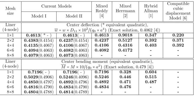
To verify the accuracy of the newly developed plate bending models, solutions obtained with the new models are compared with those of the existing models [1, 2, 6] and analytic solutions. First, the linear solutions of the mixed CPT models will be discussed by comparing the results obtained with displacement based model [4, 6].
The comparison of the results of the various models under the simple support I (SS1) and clamped (CC) boundary conditions are given in Tables 1 and 2. For the simple support boundary condition (SS1), Model II showed best accuracy for the center vertical deflection, while Model I provided better accuracy for the center bending moment, as shown in Table 1. For the clamped (CC) boundary condition, the Model I showed best accuracy both for the center vertical deflection and the center bending moment as shown in Table 2. By including
the shear forces (i.e., Vx and Vy) as nodal values in Model I, more accurate center bending
moment and center vertical deflection were obtained.
Table 1 Comparison of the linear solution of various CPT Models, isotropic (ν=0.3) square plate, simple supported (SS1).
Mesh size
Current Models Mixed
Reddy [4]
Mixed Herrmann
[2]
Hybrid Allman
[1]
Compatible cubic displacement
Model [6]
Model I Model II
Liner (4-node)
Center deflection (* equivalent quadratic), w=w×D11×102/(q0×a4)(Exact solution, 0.4062 [4])
1×1 0.4613( * - ) 0.4613( - ) 0.4613 0.9018 0.347 0.220
2×2 0.4383(0.4154) 0.4237(0.4154) 0.4237 0.5127 0.392 0.371
4×4 0.4135(0.4067) 0.4106(0.4067) 0.4106 0.4316 0.403 0.392
6×6 0.4094(0.4063) 0.4082(0.4063) 0.4082 0.4172 -
-8×8 0.4079(0.4063) 0.4073(0.4063) - - -
-Liner (4-node)
Center bending moment (equivalent quadratic), M =M×10/(q0×a2)(Exact solution, 0.479 [4])
1×1 0.7196( - ) 0.7196( - ) 0.7196 0.328 0.604
-2×2 0.5029(0.4906) 0.5246(0.4096) 0.5246 0.446 0.515
-4×4 0.4850(0.4797) 0.4892(0.4796) 0.4892 0.471 0.487
-6×6 0.4816(0.4790) 0.4834(0.4790) 0.4834 0.476 -
-8×8 0.4804(0.4788) 0.4814(0.4789) - - -
Table 2 Comparison of the linear solution of various CPT Models, isotropic (ν=0.3) square plate, clamped
(CC).
Mesh size
Current Models Mixed
Reddy [4]
Mixed Herrmann
[2]
Hybrid Allman
[1]
Compatible cubic displacement
Model [6]
Model I Model II
Liner (4-node)
Center deflection (* equivalent quadratic), w=w×D11×102/(q0×a4)(Exact solution,0.1265[4])
1×1 0.1576(* - ) 1.6644( - ) 1.6644 0.7440 0.087 0.026
2×2 0.1502(0.1512) 0.1528(0.1512) 0.1528 0.2854 0.132 0.120
4×4 0.1310(0.1279) 0.1339(0.1278) 0.1339 0.1696 0.129 0.121
6×6 0.1284(0.1268) 0.1299(0.1268) 0.1299 0.1463 -
-8×8 0.1265(0.1265) 0.1270(0.1266) - - -
-Liner (4-node)
Center bending moment (equivalent quadratic), M =M×10/(q0×a2)(Exact0.230[4])
1×1 0.4918( - ) 0.5193( - ) 0.5193 0.208 0.344
-2×2 0.2627(0.2552) 0.3165(0.2552) 0.3165 0.242 0.314
-4×4 0.2354(0.2312) 0.2478(0.2310) 0.2478 0.235 0.250
-6×6 0.2318(0.2295) 0.2374(0.2295) 0.2374 0.232 -
-8×8 0.2286(0.2290) 0.2310(0.2291) - - -
-Next, the numerical results of the Model III and IV are compared with the results of Reddy’s mixed model [4] in Table 3. The mixed model developed by Reddy [4] included bending moments as independent nodal value in the finite element model, while current Model
III and IV included vertical shear resultants (i.e., Qx and Qy), as independent nodal value.
Note that the difference between Model III and VI comes from the presence or absence of
membrane forces (i.e., Nxx,Nyy and Nxy) in the finite element models. Thus, the solution of
the linear bending of each model is essentially the same as shown in Table 3.
Table 3 Comparison of the current mixed FSDT linear solution with that of the other mixed model (Reddy [4]), with isotropic (ν=0.25, Ks=5/6) square plate, simple supported (SS1).
Mesh size
Current Models ReddyMixed
[4]
Current Models ReddyMixed
[4]
Model(III) Model(IV) Model III Model IV
Liner (4-node)
Center deflection, Center bending moment
w=wD11×102/(q0a4), M =M×10/(q0a2),
(Exact0.427 [5]) (Exact0.479[5])
1×1 0.4174(* - ) 0.4174( - ) 0.4264 0.6094( - ) 0.6094( - ) 0.6094
-4.2 Nonlinear analysis
A total of 12 load steps were used with the following values of the load parameter
P =q0a4/ (E22h4):
P ={ 6.25, 12.5, 25.0, 25.0, 25.0, 25.0, 25.0, 25.0, 25.0, 25.0, 25.0, 25.0 } (29)
A tolerance ϵ=0.01 was used for convergence in the Newton’s iteration scheme. Model I
and II was compared with the CPT displacement base model to see its non-linear behavior.
The center defection,w0, of the newly developed models are presented in Table 4. In every load
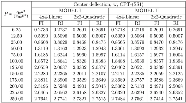
step, the converged solution was obtained within 4 iterations. Results of full integration and the reduced integration are presented in Table 4. In both models both membrane and shear locking are not severe, as judged against the published solutions, and the effect of reduced integration is not significant.
Table 4 Effect of reduced integration in Model I and II.
P = q0a
4
(E22h4)
Center deflection, w, CPT-(SS1)
MODEL I MODEL II
4x4-Linear 2x2-Quadratic 4x4-Linear 2x2-Quadratic
FI RI FI RI FI RI FI RI
6.25 0.2736 0.2737 0.2691 0.2691 0.2718 0.2719 0.2691 0.2691
12.50 0.5090 0.5096 0.5005 0.5007 0.5059 0.5064 0.5005 0.5007
25.00 0.8608 0.8629 0.8468 0.8475 0.8565 0.8579 0.8470 0.8476
50.00 1.3119 1.3163 1.2923 1.2943 1.3061 1.3093 1.2932 1.2947
75.00 1.6185 1.6244 1.5960 1.5997 1.6114 1.6157 1.5977 1.6004
100.00 1.8572 1.8641 1.8328 1.8383 1.8488 1.8539 1.8357 1.8394
125.00 2.0559 2.0637 2.0302 2.0377 2.0462 2.0521 2.0339 2.0391
150.00 2.2280 2.2365 2.2011 2.2107 2.2171 2.2235 2.2059 2.2125
175.00 2.3811 2.3900 2.3529 2.3649 2.3689 2.3757 2.3588 2.3669
200.00 2.5196 2.5289 2.4901 2.5045 2.5062 2.5133 2.4971 2.5068
225.00 2.6465 2.6562 2.6158 2.6327 2.6320 2.6394 2.6240 2.6352
250.00 2.7641 2.7741 2.7321 2.7515 2.7484 2.7561 2.7414 2.7541
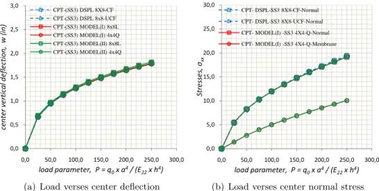
The nonlinear load vs. deflection and load vs. stress are presented in Fig. 3. For the SS3 boundary condition, both vertical deflection and stresses of Models I and II showed very close agreement with the displacement finite element model. The normal stresses and the membrane stresses were computed at points (0,0,0.5h) and (0,0,0), respectively. The 9-node quadratic element mesh showed closer agreement with the displacement FSDT model.
The nonlinear center deflection, normal and membrane stresses of Models I and II are compared with the results of the displacement model. The results are presented in Table 5.
0,0 0,5 1,0 1,5 2,0 2,5 3,0
0,0 50,0 100,0 150,0 200,0 250,0 300,0
ce
n
te
r
ve
rt
ic
a
l
d
e
fl
e
ct
io
n
,
w
(
in
)
load parameter, P = q0x a4/ (E22x h4)
CPT-(SS3) DSPL 8X8-CF CPT-(SS3) DSPL 8x8-UCF CPT-(SS3) MODEL(I) 8x8L CPT-(SS3) MODEL(I) 4x4Q CPT-(SS3) MODEL(II) 8x8L CPT-(SS3) MODEL(II) 4x4Q
(a) Load verses center deflection
0,0 5,0 10,0 15,0 20,0 25,0 30,0
0,0 50,0 100,0 150,0 200,0 250,0 300,0
S
tr
e
ss
e
s,
σxx
load parameter, P = q0x a4/ (E 22x h4)
CPT- DSPL-SS3 8X8-CF-Normal
CPT- DSPL-SS3 8X8-UCF-Normal CPT- MODEL(I) -SS3 4X4-Q-Normal CPT- MODEL(I) -SS3 4X4-Q-Membrane
(b) Load verses center normal stress
Figure 3 Plots of the membrane and normal stress of Model I, II and CPT displacement model under SS3 boundary condition.
model, as shown in Fig. 4. To see the convergence of the various models, center deflections
of previously developed models with 2×2 quadratic and 4×4 linear meshes under SS1 and SS3
boundary conditions are compared in Table 6. Every model showed good convergence with a
toleranceϵ=0.01, except for the Model IV. The Model IV showed acceptable convergence with
SS3 boundary condition but with SS1 boundary condition it took slightly more iterations to converge. This is due to the fact that plates with SS1 boundary conditions are more flexible and exhibit greater nonlinearity.
0,0 0,5 1,0 1,5 2,0 2,5 3,0
0,0 50,0 100,0 150,0 200,0 250,0 300,0
ce
n
te
r
ve
rt
ic
a
l
d
e
fl
e
ct
io
n
,
w
0
(i
n
)
load parameter, P = q0x a4/ (E22x h4)
FSDT-(SS1) DSPL 4x4Q FSDT-(SS3) DSPL 4x4Q FSDT-(SS1) MODEL(III) 8x8L FSDT-(SS1) MODEL(III) 4x4Q FSDT-(SS3) MODEL(III) 8x8L FSDT-(SS3) MODEL(III) 4x4Q
(a) Load verses center deflection
0,0 5,0 10,0 15,0 20,0 25,0 30,0
0,0 50,0 100,0 150,0 200,0 250,0 300,0
S
tr
e
ss
e
s,
σxx
load parameter, P = q0x a4/ (E22x h4)
FSDT- DSPL-SS1 4X4-Q-Normal FSDT- DSPL-SS3 4X4-Q-Normal FSDT- MODEL(III) -SS1 4X4-Q-Normal FSDT- MODEL(III) -SS1 4X4-Q-Membrane FSDT- MODEL(III) -SS3 4X4-Q-Normal FSDT- MODEL(III) -SS3 4X4-Q-Membrane
(b) Load verses center normal and mem-brane stress
Table 5 Comparison of the center deflection and normal stress of Model I and II with the CPT displacement model.
P = q0a
4
(E22 h4) Center deflection, w, CPT-(SS3)
MODEL I MODEL II DSPL DSPL
8×8-L 4×4-Q 8×8-L 4×4-Q 8×8-CF 8×8-UCF
0.00 0.0000 0.0000 0.0000 0.0000 0.0000 0.0000
25.00 0.6836 0.6774 0.6966 0.6771 0.6690 0.6700
50.00 0.9581 0.9501 0.9743 0.9497 0.9450 0.9460
75.00 1.1388 1.1296 1.1572 1.1293 1.1270 1.1280
100.00 1.2775 1.2675 1.2977 1.2672 1.2670 1.2680
125.00 1.3919 1.3813 1.4137 1.3809 1.3830 1.3830
150.00 1.4902 1.4791 1.5134 1.4787 1.4830 1.4830
175.00 1.5770 1.5654 1.6015 1.5650 1.5710 1.5710
200.00 1.6552 1.6432 1.6809 1.6428 1.6510 1.6510
225.00 1.7265 1.7142 1.7533 1.7138 1.7240 1.7240
250.00 1.7923 1.7796 1.8201 1.7793 1.7910 1.7910
P = q0a
4
(E22 h4) Normal stresses,σ
normal
xx (0,0,0.5h)×a2/E11, CPT-(SS3)
MODEL I MODEL II DSPL DSPL
8×8-L 4×4-Q 8×8-L 4×4-Q 8×8-CF 8×8-UCF
0.00 0.0000 0.0000 0.0000 0.0000 0.0000 0.0000
25.00 5.5195 5.5008 5.3402 5.4980 5.4260 5.4230
50.00 8.2751 8.2782 8.0297 8.2741 8.2470 8.2270
75.00 10.2633 10.2937 9.9885 10.2901 10.3090 10.2710
100.00 11.8988 11.9589 11.6072 11.9541 12.0170 11.9610
125.00 13.2682 13.4106 13.0238 13.4098 13.5130 13.4400
150.00 14.6077 14.7273 14.3036 14.7196 14.8670 14.7770
175.00 15.8033 15.9322 15.4838 15.9311 16.1170 16.0090
200.00 16.8734 17.0628 16.5872 17.0613 17.2870 17.1620
225.00 17.8924 18.1308 17.6290 18.1271 18.3930 18.2510
250.00 18.9188 19.1385 18.6199 19.1411 19.4460 19.2870
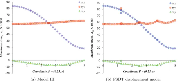
The distributions of various quantities are presented in Figs. 5 and 6. The data was post-processed inside of each element using 10 Gauss points ranging from -0.975 to 0.975, for both newly developed models (i.e., Models I and III) and FSDT displacement model. Converged
solutions of SS3 at load parameter P = 250.0 are used for the post processing.
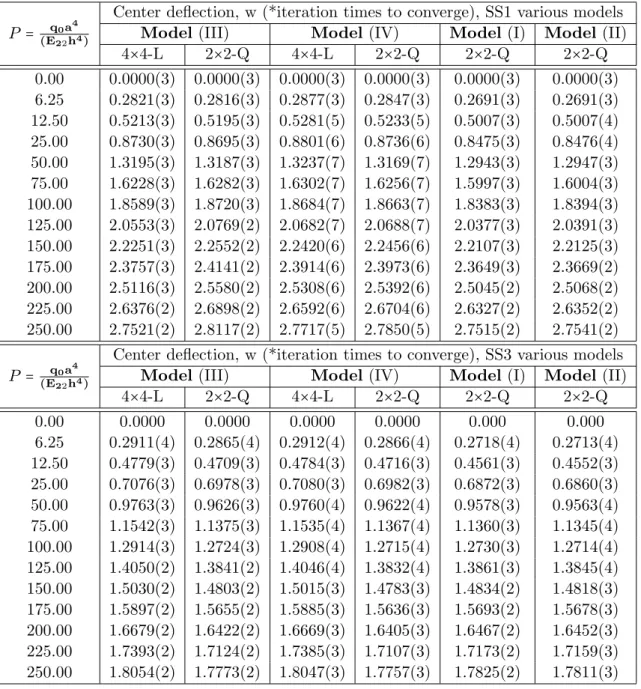
Table 6 Comparison of the convergence of Model I, II , III and IV under the SS1 and SS3 boundary conditions.
P = q0a
4
(E22h4)
Center deflection, w (*iteration times to converge), SS1 various models
Model (III) Model (IV) Model (I) Model (II)
4×4-L 2×2-Q 4×4-L 2×2-Q 2×2-Q 2×2-Q
0.00 0.0000(3) 0.0000(3) 0.0000(3) 0.0000(3) 0.0000(3) 0.0000(3)
6.25 0.2821(3) 0.2816(3) 0.2877(3) 0.2847(3) 0.2691(3) 0.2691(3)
12.50 0.5213(3) 0.5195(3) 0.5281(5) 0.5233(5) 0.5007(3) 0.5007(4)
25.00 0.8730(3) 0.8695(3) 0.8801(6) 0.8736(6) 0.8475(3) 0.8476(4)
50.00 1.3195(3) 1.3187(3) 1.3237(7) 1.3169(7) 1.2943(3) 1.2947(3)
75.00 1.6228(3) 1.6282(3) 1.6302(7) 1.6256(7) 1.5997(3) 1.6004(3)
100.00 1.8589(3) 1.8720(3) 1.8684(7) 1.8663(7) 1.8383(3) 1.8394(3)
125.00 2.0553(3) 2.0769(2) 2.0682(7) 2.0688(7) 2.0377(3) 2.0391(3)
150.00 2.2251(3) 2.2552(2) 2.2420(6) 2.2456(6) 2.2107(3) 2.2125(3)
175.00 2.3757(3) 2.4141(2) 2.3914(6) 2.3973(6) 2.3649(3) 2.3669(2)
200.00 2.5116(3) 2.5580(2) 2.5308(6) 2.5392(6) 2.5045(2) 2.5068(2)
225.00 2.6376(2) 2.6898(2) 2.6592(6) 2.6704(6) 2.6327(2) 2.6352(2)
250.00 2.7521(2) 2.8117(2) 2.7717(5) 2.7850(5) 2.7515(2) 2.7541(2)
P = q0a
4
(E22h4)
Center deflection, w (*iteration times to converge), SS3 various models
Model (III) Model (IV) Model (I) Model (II)
4×4-L 2×2-Q 4×4-L 2×2-Q 2×2-Q 2×2-Q
0.00 0.0000 0.0000 0.0000 0.0000 0.000 0.000
6.25 0.2911(4) 0.2865(4) 0.2912(4) 0.2866(4) 0.2718(4) 0.2713(4)
12.50 0.4779(3) 0.4709(3) 0.4784(3) 0.4716(3) 0.4561(3) 0.4552(3)
25.00 0.7076(3) 0.6978(3) 0.7080(3) 0.6982(3) 0.6872(3) 0.6860(3)
50.00 0.9763(3) 0.9626(3) 0.9760(4) 0.9622(4) 0.9578(3) 0.9563(4)
75.00 1.1542(3) 1.1375(3) 1.1535(4) 1.1367(4) 1.1360(3) 1.1345(4)
100.00 1.2914(3) 1.2724(3) 1.2908(4) 1.2715(4) 1.2730(3) 1.2714(4)
125.00 1.4050(2) 1.3841(2) 1.4046(4) 1.3832(4) 1.3861(3) 1.3845(4)
150.00 1.5030(2) 1.4803(2) 1.5015(3) 1.4783(3) 1.4834(2) 1.4818(3)
175.00 1.5897(2) 1.5655(2) 1.5885(3) 1.5636(3) 1.5693(2) 1.5678(3)
200.00 1.6679(2) 1.6422(2) 1.6669(3) 1.6405(3) 1.6467(2) 1.6452(3)
225.00 1.7393(2) 1.7124(2) 1.7385(3) 1.7107(3) 1.7173(2) 1.7159(3)
250.00 1.8054(2) 1.7773(2) 1.8047(3) 1.7757(3) 1.7825(2) 1.7811(3)
Displacement based FSDT Model III (FSDT) - 4 ⅹ4 Q Model I (CPT) - 4 ⅹ4 Q
-20 -10 0 10 20 30 40 50 60 70 80 90
0 1 2 3 4 5
M
e
m
b
ra
n
e
st
re
ss
,
x
x
X
1
0
0
0
0
Coordinate, P = (0.25, y)
xx
yy
xy
(a) Model III
-20 -10 0 10 20 30 40 50 60 70 80 90
0 1 2 3 4 5
M
em
b
ra
n
e
st
re
ss
,
x
x
X
1
0
0
0
0
Coordinate, P = (0.25, y)
xx
yy
xy
(b) FSDT displacement model
Figure 6 Plots of the non-linear membrane stresses of Model III and FSDT displacement model along thex
= 2.5.
-8 -6 -4 -2 0 2 4 6 8 10 12 14
0 1 2 3 4 5
B
en
d
in
g
M
o
m
en
ts
X
1
0
0
0
0
Coordinates, P = ( 2.5, y)
Myy
Mxy
Mxx
(a) Model III
-8 -6 -4 -2 0 2 4 6 8 10 12 14
0 1 2 3 4 5
B
en
d
in
g
M
o
m
en
ts
X
1
0
0
0
0
Coordinates, P = ( 2.5, y)
Myy
Mxy
Mxx
(b) FSDT displacement model
Figure 7 Plots of the non-linear bending moments of Model III and FSDT displacement model along thex= 2.5.
5 CONCLUSIONS
In this study, advantages and disadvantages of newly developed nonlinear finite element models of plate bending are investigated. In almost every case, newly developed mixed plate bending models provided better accuracy for linear and nonlinear solutions of deflections and stress resultants. Model IV showed poor convergence compared with other models because of the absence of typical displacement variables. An important observation of the present study is that the mixed models do not experience significant locking.
requirements for the transverse deflection in CPT and the increase of the accuracy for the stress resultants. Of course, there is a slight increase in computational cost due to the increased number of degrees of freedom per node.
Acknowledgement. The second author gratefully acknowledges the support of this research by Army Research Office.
References
[1] D. J. Allman. Triangular finite element for plate bending with constant and linearly varying bending moments. High Speed Computing of Elastic Structures I, pages 106–136, 1971.
[2] L. R. Herrmann. Finite element bending analysis for plates. J. Engng. Mech. Div. , ASCE, 93(EM5), 1967.
[3] N. S. Putcha and J. N. Reddy. A refined mixed shear flexible finite element for the nonlinear analysis of laminated plates. Computers & Structures, 22(4):529–538, 1986.
[4] J. N. Reddy. Mixed finite element models for laminated composite plate. Journal of Engineering for Industry, 109:39–45, 1987.
[5] J. N. Reddy. Energy Principles and Variational Methods in Applied Mechanics. John Wiley & Sons, New York, 2 edition, 2002.
[6] J. N. Reddy. An Introduction to Nonlinear Finite Element Analysis. Oxford University Press, Oxford, New York, 2004.
[7] J. N. Reddy.Mechanics of Laminated Composite Plates and Shells : Theory and Analysis. CRC Press, Boca Raton, 2 edition, 2004.
[8] J. N. Reddy. An Introduction to the Finite Element Method. McGraw-Hill, New York, 3 edition, 2006.
[9] J. N. Reddy. Theory and Analysis of Elastic Plates and Shells. CRC Press, Boca Raton, FL, 2007.
![Figure 1 Undeformed and deformed edges in the CPT and FSDT theories (from [10]).](https://thumb-eu.123doks.com/thumbv2/123dok_br/18884370.423476/3.892.209.625.122.507/figure-undeformed-deformed-edges-cpt-fsdt-theories.webp)

![Table 3 Comparison of the current mixed FSDT linear solution with that of the other mixed model (Reddy [4]), with isotropic (ν = 0.25, K s = 5/6) square plate, simple supported (SS1).](https://thumb-eu.123doks.com/thumbv2/123dok_br/18884370.423476/19.892.85.766.765.948/table-comparison-current-linear-solution-reddy-isotropic-supported.webp)