Finding candidate locations for aerosol pollution monitoring at street level using a data-driven methodology

(1)

AMTD

8, 3321–3356, 2015

Finding candidate locations for aerosol pollution monitoring

V. Moosavi et al.

Title Page

Abstract Introduction

Conclusions References

Tables Figures

◭ ◮

Back Close

Full Screen / Esc

Printer-friendly Version Interactive Discussion

Discussion

P

a

per

|

Discussion

P

a

per

|

Discussion

P

a

per

|

Discussion

P

a

per

|

Atmos. Meas. Tech. Discuss., 8, 3321–3356, 2015 www.atmos-meas-tech-discuss.net/8/3321/2015/ doi:10.5194/amtd-8-3321-2015

This discussion paper is/has been under review for the journal Atmospheric Measurement Techniques (AMT). Please refer to the corresponding final paper in AMT if available.

Finding candidate locations for aerosol

pollution monitoring at street level using

a data-driven methodology

V. Moosavi1,2, G. Aschwanden2,3, and E. Velasco4

1

Chair for Computer Aided Architectural Design (CAAD), ETH Zurich, 8092 Zurich, Switzerland

2

Future Cities Laboratory, ETH Zurich, 8092 Zurich, Switzerland

3

McCaughey VicHealth Community Wellbeing Unit, Melbourne School of Population and Global Health, University of Melbourne, Australia

4

Singapore-MIT Alliance for Research and Technology (SMART), Center for Environmental Sensing and Modeling (CENSAM), Singapore

Received: 14 October 2014 – Accepted: 5 March 2015 – Published: 26 March 2015 Correspondence to: V. Moosavi (svm@arch.ethz.ch)

(2)

AMTD

8, 3321–3356, 2015

V. Moosavi et al.

Title Page

Tables Figures

◭ ◮

Back Close

Full Screen / Esc

Discussion

P

a

per

|

Discussion

P

a

per

|

Discussion

P

a

per

|

Discussion

P

a

per

|

Abstract

Finding the number and significant locations of fixed air quality monitoring stations at ground level is challenging because of the complexity of the urban environment and the large number of factors a_ffecting the pollutants concentration. Datasets of urban param-eters such as land use, building morphology and street geometry in high resolution grid 5

cells in combination with direct measurements of airborne pollutants in high frequency (1–10 s) along a reasonable number of streets can be used to interpolate concentra-tion of pollutants in a whole gridded domain and determine the optimum number of monitoring sites and best locations for a network of fixed monitors at ground level. In this context, a data-driven modeling methodology is developed based on the appli-10

cation of Self Organizing Map (SOM) to approximate the nonlinear relations between urban parameters (80 in this work) and aerosol pollution data, such as mass and num-ber concentrations measured along streets of a commercial/residential neighborhood of Singapore. Cross-validations between measured and predicted aerosol concentra-tions based on the urban parameters at each individual grid cell showed satisfying 15

results. The urban parameters used in this case proved to be an appropriate indirect measure of aerosol concentrations within the studied area. The potential locations for fixed air quality monitors are identified through clustering of areas (i.e. group of cells) with similar urban patterns. The typological center of each cluster corresponds to the most representative cell for all other cells in the cluster. In the studied neighborhood 20

four different clusters were identified and for each cluster potential sites for air quality monitoring at ground level are identified.

1 Introduction

Air quality monitoring is needed to guide regulations for public health protection (Craig et al., 2008). At city scale air quality monitoring is performed through networks of mon-25

(3)

sta-AMTD

8, 3321–3356, 2015

V. Moosavi et al.

Title Page

Tables Figures

◭ ◮

Back Close

Full Screen / Esc

Discussion

P

a

per

|

Discussion

P

a

per

|

Discussion

P

a

per

|

Discussion

P

a

per

|

tions are placed above the urban canopy layer, where pollution measurements are not directly impacted by local emissions or obstructed wind flow (i.e. adjacent build-ings). Usually rooftops provide adequate monitoring locations. They provide informa-tion about the average urban ambient polluinforma-tion at district scale to which the general population is exposed, which is used for both, regulatory and advisory purposes (Hidy 5

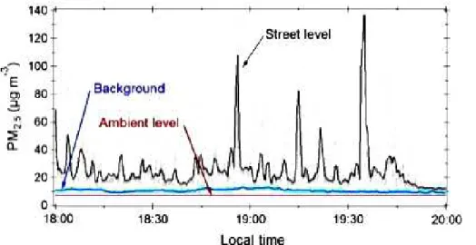
and Pennell, 2010). However, the ambient pollutants reported by these stations do not always represent the pollution to which people are exposed during their daily activities (Nerriere et al., 2005). The highest outdoor exposure to pollutants for many dwellers occurs while commuting or carrying out activities in proximity to emission sources at ground level (e.g. walking along busy streets). Figure 1 contrasts the di_fference be-10

tween concentrations of particles measured along the streets and at a site over the urban canopy layer of the neighborhood of Singapore used as a case study in this work.

Despite the stark difference between ambient and ground level pollution concentra-tions, monitoring networks include only a few ground level monitoring stations with the 15

purpose of characterizing tra_ffic emissions rather than for policy advisory. Considering the urban heterogeneity in terms of land use, buildings morphology and distribution of emission, the deployment of comprehensive monitoring networks at ground level is hampered by the required large number of monitors and their associated costs (i.e. equipment, operation and maintenance). To overcome this limitation and expand ex-20

isting air quality monitoring networks a new method is presented that determines the minimum number of ground level monitoring stations and their best potential locations. Modeling techniques, such as computational fluid dynamics (CFD) and large eddy simulation (LES) have been used to investigate the dispersion and distribution of pollu-tants under the urban canopy (e.g. Li et al., 2006; Tominaga and Stathopoulos, 2013). 25

(4)

AMTD

8, 3321–3356, 2015

V. Moosavi et al.

Title Page

Tables Figures

◭ ◮

Back Close

Full Screen / Esc

Discussion

P

a

per

|

Discussion

P

a

per

|

Discussion

P

a

per

|

Discussion

P

a

per

|

With recent advancements in computational and sensing technologies, data-driven approaches, also known as inverse or empirical modeling are an alternative to solve the problem of modeling in complex systems (Kolehmainen et al., 2001; Voukantsis et al., 2010), such as those, imposed by the urban heterogeneity on the distribution of air pol-lutants at street level. The basic idea of these models is that if there are underlying rules 5

controlling a system they can be found from a set of data by means of statistical and probabilistic methods. Therefore, with a statistically reasonable amount of air pollution observations and data on urban parameters, a data-driven mathematical model can be constructed to interpolate the pollutants concentration to a whole gridded domain with an acceptable level of accuracy. However, these models are not necessarily identifying 10

the causal elements as the source of emission, but identify a reasonable robust system of elements, based on the measured factors, that correlate with emissions.

Considering the number of potential urban parameters, controlling the pollution dis-tribution at ground level the modeling challenge turns into the challenge to identify functions that describe the nonlinear relations between the urban parameters and con-15

centration of atmospheric pollutants. This view inverts the problem of modeling from a deductive and theory-grounded approach to an inductive and data-driven approach as it is similarly described in Inverse Problem Theory (Tarantola, 2005).

In this work, Self Organizing Map (SOM) as a data-driven modeling approach is applied to find the association between particulate matter concentrations at the ground 20

level and urban parameters in its vicinity. The model (the trained SOM) is then applied to approximate the concentration of pollutants in a whole gridded domain based on the urban parameters of each particular cell. The resulting maps showing the spatial distribution of concentration of pollutants are expected to provide valuable information for epidemiological and risk assessments, as well as to identify hot spots of pollution. 25

(5)

AMTD

8, 3321–3356, 2015

V. Moosavi et al.

Title Page

Tables Figures

◭ ◮

Back Close

Full Screen / Esc

Discussion

P

a

per

|

Discussion

P

a

per

|

Discussion

P

a

per

|

Discussion

P

a

per

|

The proposed data-driven model is tested using a dataset of over 80 urban param-eters and high frequency (Either 1 or 10 s) measurements of aerosol pollution along a reasonable number of streets in a heterogeneous residential/commercial neighbor-hood of Singapore, selected as a case study. Fine-grained urban parameters are spa-tially distributed in grid cells of 100 m×100 m. The selected parameters include informa-5

tion on street networks, land-use patterns, demographics, vehicular traffic, building and street topology, etc. The aerosol pollution measurements were performed using a set of portable and battery operated sensors. The measured variables were mass concen-tration of particles with aerodynamic diameters≤10, 2.5 and 1 µm (PM₁₀, PM_2.5 and PM₁), particle number concentration (PN), active surface area (ASA), and mass con-10

centrations of black carbon (BC) and particle-bound polycyclic aromatic hydrocarbons (pPAHs).

Note that the proposed methodology is not a receptor model and does not determine any source apportionment. Receptor models utilize chemical measurements to calcu-late the relative contributions from major sources at specific locations (e.g. Viana et al., 15

2008).

The article first describes the main features of SOM methodology and its capabili-ties for multidimensional data visualization, nonlinear function approximation, and data clustering. Then the urban parameters and aerosol pollution measurements are in-troduced. The application of SOM to our case is presented in three sections. The first 20

section describes the application of SOM as a nonlinear function approximation method between urban parameters and measured aerosol concentrations. The efficiency of the approximation functions is evaluated through cross-validations between predicted and observed data. The second section explains the application of SOM to interpolate the measured pollution data from selected grid cells to the complete gridded domain. The 25

(6)

AMTD

8, 3321–3356, 2015

V. Moosavi et al.

Title Page

Tables Figures

◭ ◮

Back Close

Full Screen / Esc

Discussion

P

a

per

|

Discussion

P

a

per

|

Discussion

P

a

per

|

Discussion

P

a

per

|

stations for each one of the identified types of urban patterns (i.e. the detected clus-ters) are indicated in a final map showing also the representativeness of each grid cell within its respective cluster.

2 Methods

This section starts with a brief description of SOM as a data-driven modeling approach. 5

The following section describes the selected neighborhood of Singapore as the study area and provides details of the urban parameters, used for model evaluation. Then, the aerosol pollution measurements are introduced.

2.1 Self Organizing Map

Self Organizing Map is a data driven modeling method, introduced by Kohonen (1982). 10

From a mathematical point of view, SOM acts as a nonlinear data transformation, in which data from a high-dimensional space is transformed to a low-dimensional space (usually a space of two or three dimensions), while the topology of the original high dimensional space is preserved. Topology preservation means that if two data points are similar (i.e. close) in the high-dimensional space, they are necessarily close in the 15

low-dimensional space. This low-dimensional space, which is normally represented by a planar grid with a fixed number of points, is called a map. Each node of this map has its own coordinates (xi1,xi2) and a high-dimensional vector (Wi ={wi1,. . .,win}) where

the original observed data arendimensional vectors.

In comparison with other data transformation methods, SOM has the advantage of 20

(7)

AMTD

8, 3321–3356, 2015

V. Moosavi et al.

Title Page

Tables Figures

◭ ◮

Back Close

Full Screen / Esc

Discussion

P

a

per

|

Discussion

P

a

per

|

Discussion

P

a

per

|

Discussion

P

a

per

|

In the field of environmental modeling, data-driven methods such as supervised neu-ral networks (e.g. Multi Layer Perceptron Learning), Support Vector Machines (SVM) and time series forecasting methods such as ARIMA, have been previously applied based on the availability of massive measurements (e.g. Kolehmainen et al., 2000, 2001). In a recent study Nguyen et al. (2014) used low-resolution satellite images in 5

combination with SVM to estimate aerosol concentration at ground level from urban surfaces. Although their approach does not require direct measurements, it cannot identify the influence of urban parameters on the aerosol concentration, in contrast to our approach based on SOM. Similarly, Hirtl et al. (2014) used satellite images, ground-based measurements and the support vector regression method to improve air quality 10

forecasts at regional scale.

In summary, SOM is a generic, robust and powerful method that has been employed in several application domains (Kohonnen, 2013). It can be used for visualization of high-dimensional data and data exploration (Kolehmainen, 2004), state space model-ing and clustermodel-ing (Biermodel-inger, 2013) and most importantly, as a nonlinear function ap-15

proximation method without reducing the complexity of the system (Barreto and Souza, 2006).

2.2 Study area and urban parameters

The availability of parameters such as urban topology, land use, vehicular traffic, roads dimensions, etc. at fine spatial resolution makes Singapore a suitable place to inves-20

tigate the influence of those parameters in the air quality at ground level. For the se-lected domain of 35.1 km2, divided in cells of 100 m×100 m, 80 urban parameters were tested. The main categories of parameters are listed in Table 1. The complete list of parameters is provided in the Supplement.

Figure 2 shows the urban area, selected to test the data-driven method proposed 25

(8)

AMTD

8, 3321–3356, 2015

V. Moosavi et al.

Title Page

Tables Figures

◭ ◮

Back Close

Full Screen / Esc

Discussion

P

a

per

|

Discussion

P

a

per

|

Discussion

P

a

per

|

Discussion

P

a

per

|

Little India, which is characterized by two types of building typologies: shop-houses and residential towers. Shop-houses are multifunctional row houses of 3–5 stories, while the residential towers are up to 30 stories and can be built on a multi-story base with retail function. Rochor contains multiple urban land uses that range from residential to small-scale industrial workshops. The urban parameters used to train SOM were those 5

listed in the land use section of the Singapore Master Plan 2008 within each grid cell. Land use is derived as the number of square meters for each category.

The studied area is formed by di_fferent street layouts. Some roads are eight-lane transit streets, others shopping streets or back lanes only used for service functionality (e.g. garbage collection). To identify the individual street typology, different graph mea-10

sures (Hillier et al., 1976) were applied to the street graph encompassing the entire city-state of Singapore with different distance ranges to identify the major and minor roads.

2.3 Particles pollution measurements

For the evaluation of the data-driven method, proposed here we measured a number of 15

variables that characterize the aerosols pollution at ground level. Particles were chosen among the typical monitored air pollutants in cities because they are responsible for driving the worst air quality conditions in Singapore, as well as in many other cities (Velasco and Roth, 2012).

The aerosol pollution data were collected at ground level along streets, alleys and 20

public areas of Rochor and from a site, placed above the urban canopy (a balcony in a 28th floor) called thereafter the background site. The purpose of this site was to mea-sure particles concentrations at ambient level, as typical monitoring stations do. The route followed during the ground measurements and the location of the background site is shown in Fig. 2. The ground level route was designed to cover as much as possible 25

the different land uses and urban topologies of the selected neighborhood.

(9)

Moni-AMTD

8, 3321–3356, 2015

V. Moosavi et al.

Title Page

Tables Figures

◭ ◮

Back Close

Full Screen / Esc

Discussion

P

a

per

|

Discussion

P

a

per

|

Discussion

P

a

per

|

Discussion

P

a

per

|

tors (TSI 8534) to measure size segregated mass-fraction concentrations (PM₁, PM_2.5 and PM₁₀) at ground level and at the background site. Similarly, two handheld Con-densation Particle Counters (TSI 3007) were used to measure the PN concentration (only particles with a diameter<1 µm). Concentrations of BC and pPAHs, and the joint ASA of all particles were only measured at ground level using a Micro-Aethalometer 5

(AE51, AethLabs), a Photoelectric Aerosol Sensor (Ecochem Analytics PAS-2000 CE), and a Diffusion Charging Sensor (Ecochem Analytics DC-2000 CE), respectively. All sensors were synchronized and programmed for 1 s readings, with the exception of the sensors measuring pPAHs and ASA, which were programmed for 10 s readings. For the ground level measurements, the instruments measuring mass and number concentra-10

tions were hand carried near breathing height, while the other instruments were carried in a backpack with sampling line inlets at the same height. A Global Positioning System (GPS) was used to geo-reference the aerosol pollution readings. Additional information about the instruments and data post-processing is provided in the Supplement.

The measurements were limited to the evening period from 18:00 to 20:00 h on 15

weekdays. Public transport data from the surrounding bus and subway stations (see Fig. 2) showed that this is the period of major influx of people, and therefore of major interest from a health risk point of view. The ground level route of 3.5 km was cov-ered 20 times along 10 days of June 2013. None of the measurement days were af-fected by rain or smoke-haze from wildfires in neighboring islands (e.g. Sumatra and 20

Kalimantan). Constant meteorological conditions, as well as constant intensity of an-thropogenic activities (i.e. aerosol emissions) were assumed during the two hours of measurements.

Using the location of each measurement, obtained by the GPS readings that were properly synchronized with the particle sensors, an identification flag was assigned to 25

each measurement point using as reference the closest grid cell and its corresponding urban parameters.

(10)

AMTD

8, 3321–3356, 2015

V. Moosavi et al.

Title Page

Tables Figures

◭ ◮

Back Close

Full Screen / Esc

Discussion

P

a

per

|

Discussion

P

a

per

|

Discussion

P

a

per

|

Discussion

P

a

per

|

ground-level measurements were used to train SOM. Two reasons explain this: (1) the di_fferences between the concentrations measured at ground level and the background site showed a small variability and had therefore an insignificant influence on training SOM. Statistically, the combination of a random functionf(x)=µ(x)±σand a constant functiong(x)₌cwould result inf(x)₊g(x)₌µ(x)₊c±σthat has the same variation 5

asf(x), and consequently has no effect on the function approximation problem. (2) The urban parameters are informative to explain the variations at ground level, but not at ambient level, where pollutants are usually well-mixed and chemical reactions are also important.

3 Application of SOM as a nonlinear function approximation method between 10

urban parameters and aerosol pollution data

This section describes step by step the application of SOM as a data-driven method to approximate the nonlinear functions between the urban parameters and aerosol pollution data measured at ground level. The model is validated by cross-validations between the values predicted by SOM and the measured values. The involved steps 15

are basically three:

Step 1: Data transformation from a high to a low dimensional space;

Step 2: Modeling the nonlinear functions between urban parameters and aerosol variables;

Step 3: Validation and hypothesis testing. 20

3.1 Step 1: Data transformation from a high to a low dimensional space

(11)

AMTD

8, 3321–3356, 2015

V. Moosavi et al.

Title Page

Tables Figures

◭ ◮

Back Close

Full Screen / Esc

Discussion

P

a

per

|

Discussion

P

a

per

|

Discussion

P

a

per

|

Discussion

P

a

per

|

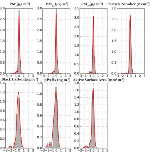
terns are observed, one linearly correlated for PM₁, PM_2.5and PM₁₀, and one nonlin-early correlated between the other variables (PN concentration, BC, pPAHs and ASA). The first pattern starts with high values in the lower-right corner of the trained map, in-creasing toward the opposite upper-left corner of the map. The second pattern shows high values in the lower-left corner increasing towards the opposite upper-right cor-5

ner. In general, when variables are grouped based on different distinct patterns, one can argue that there might be different underlying mechanisms behind the observed variables.

In this case, however the two different patterns are not surprising and can be ex-plained through the different origin of the two pollutants. In areas influenced by traffic 10

emissions, such as the district of Rochor, ultrafine particles (UFP≤100 nm in diame-ter) typically represent>90 % of PN concentration (Morawska et al., 2008). The UFP emitted directly by combustion processes or formed in the air as the hot exhaust gases are expelled from the vehicles tailpipes represent the main source of BC and pPAHs, and are strongly correlated with both PN concentration and total ASA. Because the 15

mass concentration of PM₁, PM_2.5 and PM₁₀ are several orders of magnitude larger than UFP, their concentrations do not correlate with the other measured aerosol vari-ables. Further, as within these two distinct patterns, variables have the similar patterns, we can conclude that measurements of only two aerosol parameters would have been necessary. Considering the instruments’ cost and importance of the parameters for 20

health and risk assessments, we recommend considering only measurements of BC or PN concentration in addition to PM₁for future studies.

In addition to the smooth pattern created by the SOM, the probabilistic distribution of the original data set (i.e. measurement vectors of each grid cell) can be also obtained from the trained map, as shown in Fig. 4. In this diagram, called the “hit-map”, each 25

(12)

AMTD

8, 3321–3356, 2015

V. Moosavi et al.

Title Page

Tables Figures

◭ ◮

Back Close

Full Screen / Esc

Discussion

P

a

per

|

Discussion

P

a

per

|

Discussion

P

a

per

|

Discussion

P

a

per

|

which the frequency of observed patterns (proportional to the size of the black points) can be used for resampling and simulation of the observed patterns. For a detailed description of this idea one can refer to Bieringer et al. (2013).

3.2 Step 2: Modeling the nonlinear functions between urban parameters and aerosol variables

5

The already trained SOM in combination with algorithms such as the K-Nearest Neigh-borhood (KNN) and Radial Basis Function (RBF) represents a powerful nonlinear function approximation method. For example, suppose we have a data setZ=X∪Y

in whichX ={x₁,. . .,xn} and Y ={y1,. . .,ym} under the assumption of yj=f(X). For

a new data set without y_j, a trained SOM based on data setZ, can predict the most 10

likelyyj based on the observedX (Barreto and Souza, 2006). Hence, our assumption

of nonlinear relations betweenX: {all the urban parameters} andY: {all the measured aerosol variables}. To overcome the limitation imposed by not collecting aerosol data over the complete domain (only 98 out of 3510 grid cells were monitored), we consid-ered similar aerosol concentrations for grid cells with similar urban parameters. Under 15

these assumptions the SOM was trained only with urban parameters, producing pat-terns based on the grid cells’ similarity in terms of these parameters and not of aerosol concentrations. For a grid cell with no direct measurements, the aerosol concentra-tions were predicted as the weighted average of the concentraconcentra-tions in grid cells with measurements and similar node (urban parameters) in the trained SOM. The weighted 20

averages were computed using normalized similarity values between cells of the same node. Obviously, if a projected cell presents a null similarity with any cells with measure-ments, the approach cannot predict its concentrations. The following steps describe the prediction process in detail:

1. Train a SOM based only on urban parameters (with normalized values for each 25

(13)

AMTD

8, 3321–3356, 2015

V. Moosavi et al.

Title Page

Tables Figures

◭ ◮

Back Close

Full Screen / Esc

Discussion

P

a

per

|

Discussion

P

a

per

|

Discussion

P

a

per

|

Discussion

P

a

per

|

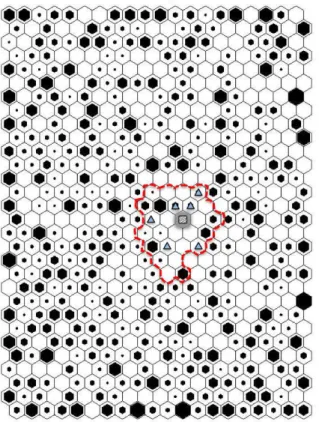
2. For each grid celli with urban parametersX_i:

2.1. Project the grid celli into the trained SOM and find theK most similar nodes in terms of urban parameters through the computation of Euclidean distances between the weighted vectors in the trained SOM andX_i (see Fig. 4).

2.2. Within the selected region of nodes (red contour in Fig. 4) find the grid cells 5

with aerosol measurements (Xr) (triangles in Fig. 4).

2.3. Calculate the normalized similarity between the selected cells and those with measurements (i.e. X_i and X_r). Similarity is calculated based on the Eu-clidean distance between each pair of high dimensional vectors.

2.4. Based on either of the two following options calculate the aerosol concentra-10

tions for celli:

– Calculate the weighted average concentrations from the selected cells with measurements. The weight is based on the normalized similarity of the urban parameters between cell i and those selected cells with measurements (i.e.Xr).

15

– If weights are close to each other with no dominant weights from a few of the selected cells, use the measurement median instead of the mean to prevent bias from extreme values, when calculating the average concen-trations. Geometric means are also an option.

With the assumption of existing relationships between urban parameters and aerosol 20

concentrations, the SOM creates a smooth map of emergent urban patterns. It is worth mentioning that in the trained SOM map, the grid cells representing the spatial surface of the neighborhood in the physical space are not necessarily placed in the same region if they do not have similar urban patterns.

The number of nodes in the SOM, defined as the width and height of the trained 25

(14)

AMTD

8, 3321–3356, 2015

V. Moosavi et al.

Title Page

Tables Figures

◭ ◮

Back Close

Full Screen / Esc

Discussion

P

a

per

|

Discussion

P

a

per

|

Discussion

P

a

per

|

Discussion

P

a

per

|

cells and 500 nodes, on average each node will represent around 7 similar grid cells, if they follow a uniform distribution). However, di_fferent grid sizes did not show to be im-portant, but very large or very small map sizes showed direct effects on the quality of the training algorithm in terms of quantization and topographic errors (Kohonen, 2001). The number of similar nodes in neighborhood search, K, is also important in order 5

to optimize the process of data-driven modeling. We tested different K values finding that values between 1 and 5 are good enough for cross-validation. Another assumption that we had in the current implementation was that all the urban parameters are equally important. However, performing the feature (i.e. urban parameter) selection and extrac-tion in a systematic manner could also optimize the training procedure as suggested 10

by Guyon and Elissee_ff (2003). Feature selection and extraction is a computationally complex problem. The number of potential combinations of urban parameters is on the order of 2n−1, wherenis the number of features including all the possible transforma-tions (e.g.z=a+b.log(x)). Methods such as the Genetic Algorithm can help to solve this optimization issue in a reasonable time (Niska et al., 2004).

15

3.3 Step 3: Validation and hypothesis testing

Before applying the SOM to predict the aerosol concentrations in the entire domain, the nonlinear relationships between the di_fferent urban parameters and aerosol con-centrations approximated by the SOM must be tested. We performed cross-validations between the predicted values and the real values to validate the proposed data-driven 20

modeling approach.

Because of the limited number of grid cells with measurements, the cross-validation was performed using 10 % of the samples in 20 iterations. This means that in each iter-ation we randomly separated 10 % of the cells with measurements from the training set and predicted their aerosol concentrations based on the remaining cells with measure-25

(15)

AMTD

8, 3321–3356, 2015

V. Moosavi et al.

Title Page

Tables Figures

◭ ◮

Back Close

Full Screen / Esc

Discussion

P

a

per

|

Discussion

P

a

per

|

Discussion

P

a

per

|

Discussion

P

a

per

|

concentrations are tightly distributed around zero with a relatively longer left tail for all of the particles, indicating a tendency to underestimate real values.

4 Application of SOM as a data-driven model to interpolate concentrations of aerosols in a gridded domain

Once the cross-validation has demonstrated satisfying results, we can proceed to in-5

terpolate the aerosol concentrations in the complete gridded domain. The interpolation methodology is essentially the same as the methodology used in the previous section for the cross-validation. The only difference is the addition of a confidence measure for the predicted concentrations. This confidence measure is based on the level of similar-ity between the urban parameters and grid cells with measurements. If no similar grid 10

cell with direct measurements is available for a particular set of grid cells with a similar urban pattern, a null confidence value will be obtained and no concentration will be predicted. In our study case, this situation occurred for regions with no urban similarity with the region where the measurements were performed. The confidence value for each cell was computed following the next steps:

15

1. The grid cells from the complete domain are divided into cells with measured data (X_M) and no measured data (X_NM).

2. The X_M cells are projected into the trained SOM to calculate the Euclidean dis-tance of each grid cell (disti) with itsK most similar nodes of SOM.

3. The median of the calculated distances forX_Mcells is used as a norm for theX_NM

20

cells, (called, the norm_dist). If the Euclidian distance for aX_NMcell is smaller or equal to this norm, the confidence will be one, in contrast if it is larger (i.e. less similarity with theX_M cells) the confidence will tend to zero. The confidence value forX_NMcells is computed as:

(16)

AMTD

8, 3321–3356, 2015

V. Moosavi et al.

Title Page

Tables Figures

◭ ◮

Back Close

Full Screen / Esc

Discussion

P

a

per

|

Discussion

P

a

per

|

Discussion

P

a

per

|

Discussion

P

a

per

|

Figure 6 shows the confidence values of each grid cell overlaid on a map of the stud-ied domain. As expected, the cells with high confidence values were those with similar patterns to cells with measured data. The distribution of cells with confidence values

>0.5 are relatively equally distributed over the built-up regions. Regions with null confi-dence correspond primarily to open spaces, such as public parks where measurements 5

were not conducted. In general, we can affirm that the proposed method is capable of interpolating aerosol pollution data at ground level within the built-up areas of a hetero-geneous neighborhood of 35.1 km2using measured data from less than 3 of the total gridded domain.

5 Potential locations for fixed monitors based on clusters of grid cells with 10

similar urban patterns

Similar to previous sections, after the good cross-validation results between the pre-dicted values by the nonlinear approximations and the measured aerosol pollution data, we can apply a clustering algorithm based on the urban parameters to determine the optimum number of fixed monitoring sites and their best locations (grid cells) in terms 15

of representativeness and maximum information gain over the whole domain.

Clustering algorithms have the task of finding the optimum number of groups from a given data set. The members (i.e. grid cells) of a group must be as much as possible similar to each other and dissimilar to the members of other groups. Each cluster must represent an individual group with a specific set of parameters. The clustering algorithm 20

must also be capable of identifying the most informative (representative) members of that cluster within each cluster.

TheK means clustering algorithm is frequently used in combination with a SOM. The SOM acts like a first step filtering and smoothing of the data points and thenK means is applied to nodes of the trained SOM, knowing the number of clusters in advance. 25

(17)

AMTD

8, 3321–3356, 2015

V. Moosavi et al.

Title Page

Tables Figures

◭ ◮

Back Close

Full Screen / Esc

Discussion

P

a

per

|

Discussion

P

a

per

|

Discussion

P

a

per

|

Discussion

P

a

per

|

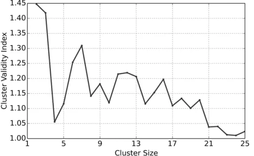
four clusters are enough for the whole gridded domain. It means that four main types of urban settings define the neighborhood of Rochor. As shown in Fig. 7, the clustering index (a metric to evaluate the clusters compactness and separation) decreases dras-tically with four clusters, but more clusters do not represent any major improvement.

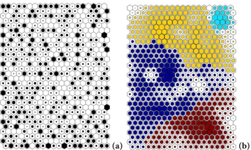
Figure 8a shows the distribution of grid cells within the trained map of SOM. The 5

size of the black spot is proportional to the number of training data in each node. After applying the K means clustering algorithm the cells grouped in four clusters can be observed in Fig. 8b. The size of the internal spots indicates the representativeness degree of the cells to their clusters. The centroid point of each cluster (the mean or median vector across all the dimensions) can be considered as its most representative 10

point. In this context, the grid cells with the highest representativeness degree within each cluster should be considered as candidate locations for monitoring air quality stations.

6 Results

The proposed methodology developed in this work offers two outcomes of potential 15

relevance for the air quality management in cities. Maps showing the spatial distribution of aerosol concentrations at ground level within the whole gridded domain represent the first outcome. The second outcome and the main goal of this work is to find the optimum number of fixed monitoring stations and their potential best locations to cover the di_fferent types of urban settings (i.e. clusters) of the studied neighborhood.

20

Figure 9 shows the spatial distribution of PM_2.5 within the gridded domain including measured and estimated data as an example of the first outcome. Similar to Fig. 6, the grid cells with no data correspond to cells with null interpolation confidence, where no prediction was possible due to the lack of similarity in terms of urban parameters with the grid cells with direct measurements. Constraining the analysis to grid cells 25

(18)

AMTD

8, 3321–3356, 2015

V. Moosavi et al.

Title Page

Tables Figures

◭ ◮

Back Close

Full Screen / Esc

Discussion

P

a

per

|

Discussion

P

a

per

|

Discussion

P

a

per

|

Discussion

P

a

per

|

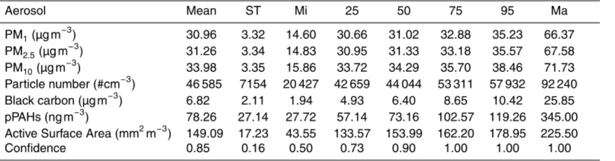
evening period from 18:00 to 20:00 h. This concentration is 1.25 times higher than the 24 h average concentration of 25 µg m−3recommended as guideline by the World Health Organization (WHO). Similarly, only 10 % of the grid cells report concentrations below the WHO guideline and 75 % are higher than 31.0 µg m−3. In comparison with the average concentration of 18.8 µg m−3 measured at the background site, only two 5

cells present smaller concentrations. Table 3 shows detailed statistics of the aerosol concentrations predicted for the whole gridded domain.

Although the measurements were conducted during the period of major influx of people, and therefore of major interest from a health risk point of view, the nonlinear relations between urban parameters and aerosol pollution data obtained by SOM can-10

not be representative for the whole diurnal course. They are only representative of the rush-hour period monitored. The nonlinear relationships will vary throughout the day as a consequence of the variability in the emissions’ intensity within the studied neighborhood. However, the aerosol measurements during the evening rush-hour had the unique purpose of testing SOM. The proposed methodology is expected to be 15

used in the design of future long term studies. Maps showing the spatial distribution of pollutants concentration at ground level in fine-grained domains will provide valu-able information for epidemiological and risk assessments. We already discussed the poor ability of typical ambient monitoring stations to represent the pollution levels at the height where urban dwellers carry out the majority of their activities. This is of particular 20

concern in the ubiquitous environments a_ffected by vehicular emissions. Many epidemi-ological studies have found significant health effects due to exposure to vehicular traffic (e.g. Lipfert and Wyzga, 2008). Although these studies have investigated various expo-sure criteria, including tra_ffic intensity and proximity, control strategies have generally not yet been proposed on a widespread basis, in part due to the lack of long term air 25

(19)

AMTD

8, 3321–3356, 2015

V. Moosavi et al.

Title Page

Tables Figures

◭ ◮

Back Close

Full Screen / Esc

Discussion

P

a

per

|

Discussion

P

a

per

|

Discussion

P

a

per

|

Discussion

P

a

per

|

useful for urban planning, in particular when designing strategies to improve urban mo-bility promoting walking and cycling as means to cover the so called first and last miles (distances that commuters must cover in getting to and from public transportation).

Figure 10 summarizes the application of SOM as a data-driven method to find the optimum number of monitoring stations and their potential locations in terms of repre-5

sentativeness. The top candidate grid cell(s) for each one of the four different urban settings that form the residential/commercial neighborhood of Rochor are marked over the individual maps of each urban cluster. The grid cells were brought back to the real two-dimensional space using as reference their latitude and longitude data. The next step in the selection of sites is to visit the candidate locations and verify that enough 10

space is available for a fixed monitoring station, the security conditions and continuous access to power. If we select more than one candidate location for each cluster (say three top candidates, each selected independently), another optimization step would be necessary to find the best four monitoring stations out of 12 candidate points (three locations for four clusters) in a way to minimize the overlap between stations of di_fferent 15

clusters and maximize the total physical coverage of the monitoring stations.

7 Conclusions

The capability of SOM as a data-driven modeling method to approximate nonlinear re-lationships between multiple urban parameters and air pollution data at ground level was demonstrated using a database of urban parameters spatially distributed in high 20

resolution grid cells created with purposes different to air quality monitoring (e.g. ur-ban planning) and aerosol pollution data collected during a short field study. The good agreement between measured and predicted aerosol concentrations showed that the group of urban parameters used in this work provides a good indirect measure of aerosol pollution at ground level within the studied neighborhood. The same methodol-25

(20)

AMTD

8, 3321–3356, 2015

V. Moosavi et al.

Title Page

Tables Figures

◭ ◮

Back Close

Full Screen / Esc

Discussion

P

a

per

|

Discussion

P

a

per

|

Discussion

P

a

per

|

Discussion

P

a

per

|

The satisfying results of SOM to approximate nonlinear relationships from multidi-mensional data gave opportunity to apply SOM as a method to interpolate aerosol pollution data in a complete gridded domain, including grid cells with no direct mea-surements. In the same context, SOM in combination with a clustering algorithm was used to determine the optimum number of locations for monitoring sites to cover the 5

different urban settings or clusters forming the studied neighborhood, as well as to find their best candidate locations in terms of representativeness of urban patterns within their clusters.

The data-driven modeling methodology developed in this work must be relatively easy to implement to other urban domains if such urban parameters as street net-10

works, land-use patterns, demographics, transportation data, and building and street topology are available in databases of high spatial resolution. The aerosol pollution measurements should not represent a major cost if portable and battery-operated sen-sors are used, as in this work. We evaluated seven di_fferent aerosol parameters, but measurements only of black carbon or particle number concentration in addition to 15

PM₁would have only been necessary according to the nonlinear correlations between aerosol parameters, identified visually by SOM.

The Supplement related to this article is available online at doi:10.5194/amtd-8-3321-2015-supplement.

Acknowledgements. This research was supported by the National Research Foundation

Sin-20

(21)

AMTD

8, 3321–3356, 2015

V. Moosavi et al.

Title Page

Tables Figures

◭ ◮

Back Close

Full Screen / Esc

Discussion

P

a

per

|

Discussion

P

a

per

|

Discussion

P

a

per

|

Discussion

P

a

per

|

References

Barreto, G. A. and Souza, L. G. M.: Adaptive filtering with the self-organizing map: a perfor-mance comparison, Neural Networks, 19, 785–798, 2006.

Bieringer, P. E., Longmore, S., Bieberbach, G., Rodriguez, L. M., Copeland, J., and Hannan, J.: A method for targeting air samplers for facility monitoring in an urban environment, Atmos.

5

Environ., 80, 1–12, 2013.

Craig, L., Brook, J. R., Chiotti, Q., Croes, B., Gower, S., Hedley, A., Krewsky, D., Krupnik, A., Kryzanowski, M., Moran, M. D., Pennell, W., Samet, J. M., Schneider, J., Shortreed, J., and Williams, M.: Air pollution and public health: a guidance document for risk managers, J. Toxicol. Env. Heal. A, 71, 588–698, 2008.

10

Guyon, I. and Elisseeff, A.: An introduction to variable and feature selection, J. Mach. Learn. Res., 3, 1157–1182, 2003.

Hidy, G. M. and Pennell, W. T.: Multipollutant air quality management, J. Air Waste Manage., 60, 645–674, 2010.

Hillier, B., Leaman, A., Stansall, P., and Bedford, M.: Space syntax, Environ. Plann. B, 3, 147–

15

185, 1976.

Hirtl, M., Mantovani, S., Krüger, B. C., Triebnig, G., Flandorfer, C., Bottoni, M., and Cavicchi, M.: Improvement of air quality forecasts with satellite and ground based particulate matter ob-servations, Atmos. Environ., 84, 20–27, 2014.

Kohonen, T.: Self-organized formation of topologically correct feature maps, Biol. Cybern., 43,

20

59–69, 1982.

Kohonen, T.: Self-Organizing Maps, Vol. 30, Springer, 2001.

Kohonen, T.: Essentials of the self-organizing map, Neural Networks, 37, 52–65, 2013.

Kukkonena, J., Partanena, L., Karppinena, A., Ruuskanenb, J., Junninenb, H., Kolehmainenb, M., Niskab, H., Dorlingc, S., Chattertonc, T., Foxalld, R., and Cawleyd, G.: Extensive

evalua-25

tion of neural network models for the prediction of NO₂and PM₁₀concentrations, compared with a deterministic modeling system and measurements in central Helsinki, Atmos. Environ., 37, 4539–4550, 2003.

Kolehmainen, M., Martikainen, H., Hiltunen, T., and Ruuskanen, J.: Neural networks and peri-odic components used in air quality forecasting, Atmos. Environ., 35, 815–825, 2001.

30

(22)

AMTD

8, 3321–3356, 2015

V. Moosavi et al.

Title Page

Tables Figures

◭ ◮

Back Close

Full Screen / Esc

Discussion

P

a

per

|

Discussion

P

a

per

|

Discussion

P

a

per

|

Discussion

P

a

per

|

Li, X. X., Liu, C. H., Leung, D. Y. C., and Lam, K. M.: Recent progress in CFD modeling of wind field and pollutant transport in street canyons, Atmos. Environ., 40, 5640–5658, 2006. Li, X. X., Britter, R. E., Norford, L. K., Koh, T.-Y., and Entekhabi, D.: Flow and pollutant transport

in urban street canyons of different aspect ratios with ground heating: large Eddy Simulation, Bound.-Lay. Meteorol., 142, 289–304, 2012.

5

Lipfert, F. and Wyzga, R. E.: On exposure and response relationships for health effects associ-ated with exposure to vehicular traffic, J. Expo. Sci. Env. Epid., 18, 588–599, 2008.

Morawska, L., Ristovski, Z., Jayaratne, E., R., Keogh, D. U., and Ling, X.: Ambient nano and ultrafine particles from motor vehicle emissions: characteristics, ambient processing and im-plications on human exposure, Atmos. Environ., 42, 8113–8138, 2008.

10

Nerriere, É., Zmirou-Navier, D., Blanchard, O., Momas, I., Ladner, J., Le Moullec, Y., Person-naz, M. B., Lameloise, P., Delmas, V., Target, A., and Desqueyroux, H.: Can we use fixed ambient air monitors to estimate population long-term exposure to air pollutants? The case of spatial variability in the Genotox ER study, Environ. Res., 97, 32–42, 2005.

Nguyen, T. N. T., Ta, V. C., Le, T. H., and Mantovani, S.: Particulate matter concentration

es-15

timation from satellite aerosol and meteorological parameters: data-driven approaches, in: Knowledge and Systems Engineering, Springer International Publishing, 351–362, 2014. Niska, H., Hiltunen, T., Karppinen, A., Ruuskanen, J., and Kolehmainen, M.: Evolving the neural

network model for forecasting air pollution time series, Eng. Appl. Artif. Intel., 17, 159–167, 2004.

20

Tarantola, A.: Inverse Problem Theory and Methods for Model Parameter Estimation, SIAM, 2005.

Tibshirani, R., Walther, G., and Hastie, T.: Estimating the number of clusters in a data set via the gap statistic, J. Roy. Stat. Soc. B, 63, 411–423, 2001.

Tominaga, Y. and Stathopoulos, T.: CFD simulation of near-field pollutant dispersion in the

25

urban environment: a review of current modeling techniques, Atmos. Environ., 79, 716–730, 2013.

Ultsch, A.: U*-Matrix: a Tool to Visualize Clusters in High Dimensional Data, Fachbereich Math-ematik und Informatik, 2003.

Velasco, E. and Roth, M.: Review of Singapore’s air quality and greenhouse gas emissions:

30

current situation and opportunities, J. Air Waste Manage., 62, 625–641, 2012.

(23)

AMTD

8, 3321–3356, 2015

V. Moosavi et al.

Title Page

Tables Figures

◭ ◮

Back Close

Full Screen / Esc

Discussion

P

a

per

|

Discussion

P

a

per

|

Discussion

P

a

per

|

Discussion

P

a

per

|

Vecci, R., Miranda, A. I., Kasper-Giebl, A., Maenhaut, W., and Hitzenberger, R.: Source ap-portionment of particulate matter in Europe: a review of methods and results, J. Aerosol Sci., 39, 827–849, 2008.

Voukantsis, D., Niska, H., Karatzas, K., Riga, M., Damialis, A., and Vokou, D.: Forecasting daily pollen concentrations using data-driven modeling methods in Thessaloniki, Greece, Atmos.

5

(24)

AMTD

8, 3321–3356, 2015

V. Moosavi et al.

Title Page

Tables Figures

◭ ◮

Back Close

Full Screen / Esc

Discussion

P

a

per

|

Discussion

P

a

per

|

Discussion

P

a

per

|

Discussion

P

a

per

|

Table 1.Main categories of urban parameters with influence on the aerosols concentration at ground level of the residential/commercial neighborhood of Rochor, Singapore, used as a study case.

Category Data source

Land use Singapore Master Plan 2008 Street network and connectivity Singapore Land Transport Authority Building topology NAVTEQ Building Footprint

(25)

AMTD

8, 3321–3356, 2015

V. Moosavi et al.

Title Page

Tables Figures

◭ ◮

Back Close

Full Screen / Esc

Discussion

P

a

per

|

Discussion

P

a

per

|

Discussion

P

a

per

|

Discussion

P

a

per

|

Table 2.Efficiency of SOM to approximate nonlinear relationships between urban parameters and aerosol concentrations. The cross-validation was performed using 10 % of the samples in 20 interactions as explained in the text.

Aerosol Based on median values Based on arithmetic mean variable of similar grid cells values of similar grid cells Median of Mean of Median of Mean of accuracy (%) accuracy (%) accuracy (%) accuracy (%)

PM1 92.18 85.81 93.03 87.13

PM2.5 92.16 85.87 92.98 87.21

PM10 92.64 87.27 93.21 87.20

Particle number 89.34 85.97 90.24 86.48

Black carbon 78.08 69.37 79.10 67.34

pPAHs 78.72 70.67 82.42 70.98

Active surface area 88.36 75.06 88.67 76.81

Average accuracy (%) 87.35 80.00 88.52 80.45

Min accuracy (%) 78.08 69.37 79.10 67.34

(26)

AMTD

8, 3321–3356, 2015

V. Moosavi et al.

Title Page

Tables Figures

◭ ◮

Back Close

Full Screen / Esc

Discussion

P

a

per

|

Discussion

P

a

per

|

Discussion

P

a

per

|

Discussion

P

a

per

|

Table 3.Statistics of the aerosol concentrations predicted by SOM for the complete gridded domain of the neighborhood of Rochor on weekdays during the evening rush hour (18:00– 20:00 h). The analysis considers only grid cells with measured or extrapolated data with confi-dence values≥0.5.

Aerosol Mean ST Mi 25 50 75 95 Ma

PM1(µg m−3) 30.96 3.32 14.60 30.66 31.02 32.88 35.23 66.37

PM2.5(µg m− 3

) 31.26 3.34 14.83 30.95 31.33 33.18 35.57 67.58

PM10(µg m− 3

) 33.98 3.35 15.86 33.72 34.29 35.70 38.46 71.73

Particle number (#cm−3) 46 585 7154 20 427 42 659 44 044 53 311 57 932 92 240 Black carbon (µg m−3) 6.82 2.11 1.94 4.93 6.40 8.65 10.42 25.85 pPAHs (ng m−3) 78.26 27.14 27.72 57.14 73.16 102.57 119.26 345.00 Active Surface Area (mm2m−3) 149.09 17.23 43.55 133.57 153.99 162.20 178.95 225.50

(27)

AMTD

8, 3321–3356, 2015

V. Moosavi et al.

Title Page

Tables Figures

◭ ◮

Back Close

Full Screen / Esc

Discussion

P

a

per

|

Discussion

P

a

per

|

Discussion

P

a

per

|

Discussion

P

a

per

|

Figure 1.Time series of PM2.5mass concentration measured above the urban canopy

(28)

AMTD

8, 3321–3356, 2015

V. Moosavi et al.

Title Page

Tables Figures

◭ ◮

Back Close

Full Screen / Esc

Discussion

P

a

per

|

Discussion

P

a

per

|

Discussion

P

a

per

|

Discussion

P

a

per

|

(29)

AMTD

8, 3321–3356, 2015

V. Moosavi et al.

Title Page

Tables Figures

◭ ◮

Back Close

Full Screen / Esc

Discussion

P

a

per

|

Discussion

P

a

per

|

Discussion

P

a

per

|

Discussion

P

a

per

|

(30)

AMTD

8, 3321–3356, 2015

V. Moosavi et al.

Title Page

Tables Figures

◭ ◮

Back Close

Full Screen / Esc

Discussion

P

a

per

|

Discussion

P

a

per

|

Discussion

P

a

per

|

Discussion

P

a

per

|

(31)

AMTD

8, 3321–3356, 2015

V. Moosavi et al.

Title Page

Tables Figures

◭ ◮

Back Close

Full Screen / Esc

Discussion

P

a

per

|

Discussion

P

a

per

|

Discussion

P

a

per

|

Discussion

P

a

per

|

(32)

AMTD

8, 3321–3356, 2015

V. Moosavi et al.

Title Page

Tables Figures

◭ ◮

Back Close

Full Screen / Esc

Discussion

P

a

per

|

Discussion

P

a

per

|

Discussion

P

a

per

|

Discussion

P

a

per

|

(33)

AMTD

8, 3321–3356, 2015

V. Moosavi et al.

Title Page

Tables Figures

◭ ◮

Back Close

Full Screen / Esc

Discussion

P

a

per

|

Discussion

P

a

per

|

Discussion

P

a

per

|

Discussion

P

a

per

|

(34)

AMTD

8, 3321–3356, 2015

V. Moosavi et al.

Title Page

Tables Figures

◭ ◮

Back Close

Full Screen / Esc

Discussion

P

a

per

|

Discussion

P

a

per

|

Discussion

P

a

per

|

Discussion

P

a

per

|

Figure 8. (a)Distribution of grid cells after applying the K means clustering algorithm. Each cluster is represented by a different color. The size of the internal spots indicates the represen-tativeness degree of each cell to its cluster. Cells with larger spots are more representative.(b)

(35)

AMTD

8, 3321–3356, 2015

V. Moosavi et al.

Title Page

Tables Figures

◭ ◮

Back Close

Full Screen / Esc

Discussion

P

a

per

|

Discussion

P

a

per

|

Discussion

P

a

per

|

Discussion

P

a

per

|

Figure 9.Spatial distribution of PM2.5at the studied neighborhood of Rochor during the evening

(36)

AMTD

8, 3321–3356, 2015

V. Moosavi et al.

Title Page

Tables Figures

◭ ◮

Back Close

Full Screen / Esc

Discussion

P

a

per

|

Discussion

P

a

per

|

Discussion

P

a

per

|

Discussion

P

a

per

|