Inferring Strain Mixture within Clinical
Plasmodium falciparum
Isolates from
Genomic Sequence Data
John D. O’Brien1*, Zamin Iqbal2, Jason Wendler3, Lucas Amenga-Etego2,4
1Mathematics Department, Bowdoin College, Brunswick, Maine, United States of America,2Wellcome Trust Centre for Human Genetics, University of Oxford, Oxford, Oxfordshire, United Kingdom,3Pacific Northwest National Laboratory, Richland, Washington, United States of America,4Navrongo Health Research Centre, Navrongo, Upper East Region, Ghana
Abstract
We present a rigorous statistical model that infers the structure ofP. falciparummixtures— including the number of strains present, their proportion within the samples, and the amount of unexplained mixture—using whole genome sequence (WGS) data. Applied to simulation data, artificial laboratory mixtures, and field samples, the model provides reasonable infer-ence with as few as 10 reads or 50 SNPs and works efficiently even with much larger data sets. Source code and example data for the model are provided in an open source fashion. We discuss the possible uses of this model as a window into within-host selection for clinical and epidemiological studies.
Author Summary
Since the 1960’s researchers have observed thatPlasmodium falciparuminfections, the
cause of most severe malaria, are frequently composed of several different strains of the parasite. In this work, the authors use Bayesian methods on whole genome sequence data to model the structure of these mixtures. Results from this method are consistent with pre-vious approaches but provide finer resolution of these mixtures. As whole genome data in malaria research becomes increasingly common, this work will allow researchers to delve further into the within-host dynamics of the parasite, a much-discussed but previously dif-ficult-to-access aspect of this disease.
This is aPLOS Computational BiologyMethods paper.
a11111
OPEN ACCESS
Citation:O’Brien JD, Iqbal Z, Wendler J, Amenga-Etego L (2016) Inferring Strain Mixture within Clinical
Plasmodium falciparumIsolates from Genomic Sequence Data. PLoS Comput Biol 12(6): e1004824. doi:10.1371/journal.pcbi.1004824
Editor:Sergei L. Kosakovsky Pond, Temple University, UNITED STATES
Received:August 13, 2015
Accepted:February 17, 2016
Published:June 30, 2016
Copyright:This is an open access article, free of all copyright, and may be freely reproduced, distributed, transmitted, modified, built upon, or otherwise used by anyone for any lawful purpose. The work is made available under theCreative Commons CC0public domain dedication.
Data Availability Statement:These data are available via the PF3K data release 3:www. malariagen.net/data/pf3k-3and the European Nucleotide Archive:www.ebi.ac.uk/ena. The sample numbers are included in the manuscript.
Introduction
The protozoan parasitePlasmodium falciparum(Pf) is the cause of the vast majority of fatal
malaria cases, killing at least half a million people a year [1–3]. The parasite’s ability to develop
resistance to drugs and the rapid spread of that resistance across geographically-separated
pop-ulations presents a constant threat to international control efforts [4–6]. While research has
elucidated many genetic factors this process, much of the genetic epidemiology of the parasite
—including the effective recombination rate and the rate of gene flow across populations—is
still unclear [5,7,8].
Understanding the implications of multiplicity of infection (MOI), where multiple strains
appear to be present within a single patient’s bloodstream, is a long-standing challenge [9–13].
While MOI-focused studies implicate MOI levels with a range of conditions, including clinical
severity [14], age-specific severity [15–18], parasitemia levels during pregnancy [19], and other
effects [20–23], there is no broad consensus about its role in controlling the course of an
infec-tion. Still, a wide variety of studies and genetic assays—most commonly through typing the
MSPgenes—show MOI as a regular feature of clinical Pf isolates [24–26].
WGS technologies applied to Pf extracted directly from infected patients’bloodstreams
pro-vide an unprecedented window into the structure of genetic mixture within samples [27,28].
Initial work on this data shifted focus from estimating MOI to analysis based on inbreeding
coefficients [13,29–31]. These metrics, a form ofF-statistic, give an estimate of the departure
of within-sample allele frequencies from those expected under a Hardy-Weinberg-type
equilib-rium with the ambient population. From this perspective, each patient’s bloodstream is seen as
a subpopulation comprised of an admixture of all strains in the local environment, ranging from a perfectly random sampling of all nearby strains (panmixia) to the repeated sampling of just a single strain (unmixed).
The initial study applying WGS to clinical Pf isolates from eight countries on three conti-nents showed the parasite to exhibit significant population structure at continental scales, with
the amount of subpopulation structure varying significantly among regions [27]. Employing
an F-statistic approach to measure the inbreeding coefficient from thousands of single nucleo-tide polymorphisms (SNPs), this work also argued that the degree of mixture varies signifi-cantly across populations, with highly mixed samples occurring relatively frequently in west Africa but only occasionally in Papua New Guinea. The authors suggest an association between increased levels of observed mixture and increased transmission intensity in the local environ-ment. Transmission intensity, the rate at which individuals are infected with Pf, likely deter-mines some part of the frequency of out-crossing within parasite populations and so may be
critical to understanding gene flow and strategies for resistance control [32].
In this paper, we present a statistically rigorous model that synthesizes these two distinct and previously disparate approaches to analyzing Pf clinical mixtures: assessing the number of
distinct genetic types within a sample (the MOI approach [31]) and measuring the degree of
panmixia with respect to the local population (the panmixia approach [33]). The model makes
two significant innovations: first, a reversible jump Markov Chain Monte Carlo (MCMC) implementation to capture uncertainty in the number of strains, and second the inclusion of a panmixia term to deal with unexplained variation in the mixture. This work possesses
similari-ties in character to the COIL algorithm [34], but can capture more complex mixture structure
and is geared toward analyzing WGS data (>1000 SNPs) rather than a small number of SNPs
(*50 SNPs).
This model centers around how the two sub-models—MOI and panmixia—contribute to
the observedwithin-samplenon-reference allele frequencies (WSAF) as they relate to the
popu-lation-levelnon-reference allele frequencies (PLAF). For clarity, we will deprecate the use of
(http://www.mrc.ac.uk/funding/). The funders had no role in study design, data collection and analysis, decision to publish, or preparation of the manuscript.
non-referencein front of the term allele frequency, since they are all calibrated in this fashion. We will use the acronyms WSAF to denote the within-sample allele frequency and PLAF to denote population-level allele frequency to avoid confusion about the particularly allele
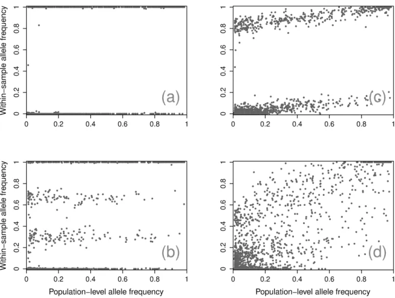
fre-quency being indicated. The goal of the model is to explain observed‘bands’that emerge when
examining SNPs WSAF as a function of their PLAF (Fig 1).
The model assumes (1) that the number of bands is a consequence of the number of distinct strains present within a sample, (2) that SNPs are unlinked, and (3) that unexplained variation is assumed to be due to a small fraction of genomes sampled under panmixia. To distinguish
from an inbreeding coefficient—a similar but distinct concept—we refer to this fraction as a
panmixia coefficient. The collection of WSAF bands then appears as a function of the finite mixture of the strains, with the slope in WSAF bands with respect to the PLAF explained by both the SNP distribution and the panmixia coefficient.
Fig 1. Example samples.Four representative samples with WSAF for each SNP plotted against the PLAF, showing an absence of mixture (a), a partially panmixed sample (b), a simple mixture (c), and a complex mixture (d).
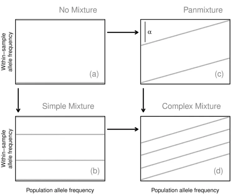
Fig 2lays out how the consequent banding patterns can arise. In the simplest case, a sample
is composed of a single, unmixed strain, and all SNPs exhibit a WSAF of zero or one (seeFig 2
(a)), based on whether they agree with the reference. Consequently, the WSAF is independent
of PLAF, leading to two flat bands at these values. We call these samples unmixed, since this is how a single strain with some divergence from the reference will appear. In the case where there are a finite number of strains mixed within a sample, then at a given SNP position some number of the strains will exhibit a reference allele and some a non-reference allele. The WSAF for that SNP is determined by the proportions of non-reference strains in the sample mixture.
Observing many SNPs displays‘bands’of constant WSAF across the PLAF. Thus, forK
com-ponent strains there are 2Kpossible combinations of biallelic states, leading to that number of
bands.
Fig 2. Model diagram.The structure of the model can be understood in terms of four related states connecting the WSAF to the PLAF: no mixture (upper left); simple mixture (lower left); panmixture (upper right); and complex mixture (lower right).αis exaggerated for explanation; realistic values are less than 0.05.
A fraction of the Pf organisms present within the blood may not be from any of the domi-nant strains. We model these as randomly sampled from the local population according to sim-ple panmixia. Observationally, this leads to a consistent change in the slope of each of the bands. To see this, consider an admixture of two distinct Pf populations: a single strain,
repre-senting 1−αof the within-sample genomes, and the remainingαthat we assume follow
pan-mixia. Theαtilt in the WSAF arises from the fact that for this proportion of organisms the
probability of sampling non-reference allele is proportional to the PLAF (Figs1(c)and2(c)).
Samples with highKappear to have additional tilt due to the higher probability of
non-refer-ence alleles occurring at high PLAF (Figs1(d)and2(d)).
The paper proceeds as follows. We first detail the structure of the WGS data, introduce some notation, and the essential mathematical structure of the model. We then present an extensive simulation study on the performance of the model, an application of the model to artificial laboratory mixtures, and an examination of its application to field isolates collected from northern Ghana. We conclude by discussing the strengths and weaknesses of the model, a means of experimental validation, and potential consequences for the etiology of clinical malaria.
Materials and Methods
Data
The field WGS data come from Illumina HiSeq sequencing applied to Pf extracted from 419 clinical blood samples collected from infected patients in the Kassena-Nankana district (KND) region of Upper East Region of northern Ghana. Collection occurred over approximately 2 years, from June 2009-June 2011. The raw sequence reads for these data are accessible through
the PF3K projecthttps://www.malariagen.net/projects/parasite/pf3k. This includes data from
the MalariaGEN Plasmodium falciparum Community Project onwww.malariagen.net/
projects/parasite/pf. On the website for this method, we provide read count data subsampled from the full data set. The artificial laboratory samples were sequenced and called per protocols
given in [35]. The raw sequence data is available through the European Nucleotide Archive
with the accessions available in theS1 Text.
The full sequencing protocol and collection regime are described in [27]. After quality
con-trol measures, all samples were examined, and following a documented protocol comparing against world-wide variation, 198,181 single-nucleotide polymorphisms (SNPs) were called
[27]. These are exclusively coding SNPs found outside of the telomeric and subtelomeric
regions that exhibit unusual structural properties. Each SNP xcall provides the number of refer-ence and non-referrefer-ence read counts observed at each variant position within the genome,
ascertained against the the 3D7 reference [36]. These data were exhaustively examined for
spu-rious heterozygosity and evidence of DNA contamination, with mixed calls verified using
time-of-flight mass spectrometry at greater than 99% accuracy [27].
For this project, we further filtered the data. First, multiallelic positions were reclassed as biallelic. We then excluded positions that exhibited no variation within the KND samples, any level of missingness (no read counts observed), or minor allele frequency less than 0.01. To remove low quality samples, we removed those with more than 4,000 SNPs missing and fewer
than 20 read counts, following an inflection point observed inS1 Fig. These cleaning measures
left 2,429 SNPs in 168 samples. These SNPs exhibit desirable properties for model inference—
high and consistent coverage across all samples—that could likely be expanded to non-coding
or less stringent cleaning standards without issue. More than 95% of the remaining samples’
neighbor-joining tree of the pairwise difference among samples (S2 Fig). The data preparation
scripts are available with the source code for the model,https://github.com/jacobian1980/
pfmix/.
Notation
Following the data preparation and cleaning, our analysis begins with a set ofN= 168 clinical
samples, each composed ofM= 2,429 SNPs. At each SNPjwithin each clinical samplei, we
observerijreads that agree with the reference genome andnijreads that do not agree. The total
number of read counts in sampleiat SNPjis thennij+rij. For a samplei, we write the
com-plete data across all SNPs asDi ¼ ½ðri1;ni1Þ; ;ðriM;niMÞ. For each SNPj, we associate a
PLAFpj. The collection of allpjwe refer to asP.
Conditional upon the number of strainsK, there are 2Kbands, indexed byr= 1, , 2K. The
full collection of bands we callQ, withqijrindicating the WSAF for sampleiat SNPjin bandr.
The probability of a SNP lying within the distinct bands across the PLAF is specified by a
mix-ture componentλr, which is a function of the PLAF detailed below. The degree of panmixia in
a sample is given byα, a value between zero and one. A complete list of the model parameters
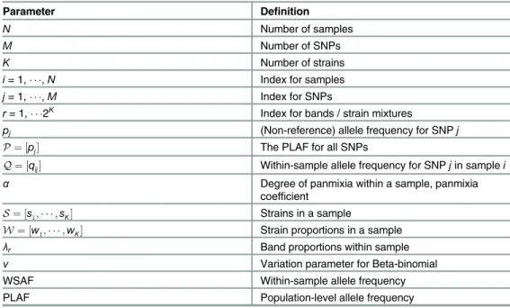
is given inTable 1.
Model
Statistically, the model takes the form of a finite mixture model with the mixture components
associated with individual bands [37,38]. We take a Bayesian approach to inference and
con-struct the model by giving an overall rationale for the decomposition of the posterior distribu-tion, and then justify the appropriate choice of probability distributions for each of the terms [39].
Table 1. Parameters and definitions for the model and its description.
Parameter Definition
N Number of samples
M Number of SNPs
K Number of strains
i= 1, ,N Index for samples
j= 1, ,M Index for SNPs
r= 1, 2K
Index for bands / strain mixtures
pj (Non-reference) allele frequency for SNPj
P¼ ½pj The PLAF for all SNPs
Q¼ ½qij Within-sample allele frequency for SNPjin samplei
α Degree of panmixia within a sample, panmixia
coefficient
S¼ ½s1; ;sK Strains in a sample
W¼ ½w1; ;wK Strain proportions in a sample
λr Band proportions within sample
ν Variation parameter for Beta-binomial
WSAF Within-sample allele frequency
PLAF Population-level allele frequency
Decomposition. We assume that samples are independent of each other and that the SNP
data for each sample depends solely on the number of bands (K), the WSAF (Q), the PLAF
(P), and a shape parameterν. As samples are treated independently, we deprecate
sample-spe-cific subscripts for the model parameters. Considering the data for a single sample,Di, the
pos-terior distribution can then be written as:
PðQ;P;W;a;n;KjDiÞ / PðDijQ;P;W;a;n;KÞ PðQ;P;W;a;n;KÞ
¼ PðDijQ;P;n;KÞ PðQ;P;n;K;W;aÞ:
ð1Þ
We also assume that the WSAF depends only on the PLAF, the panmixia coefficient, the
number of strains, and their proportions within the sample, allowing the right-hand side ofEq
(1)to be further decomposed, by noting that:
PðQ;P;n;K;W;aÞ ¼ PðQjP;n;K;W;aÞ PðP;n;K;W;aÞ: ð2Þ
While the strain proportions clearly depend on the number of strains, the remaining parame-ters we take to be independent of this value and of each other. This means that the last
right-hand side term inEq (2)becomes:
PðP;n;K;W;aÞ ¼ PðPÞ PðnÞ PðWjKÞ PðKÞ PðaÞ: ð3Þ
Substituting Eqs (2) and (3) intoEq (1), yields thefinal decomposition:
PðQ;P;W;a;n;KjDiÞ / PðDijQ;P;n;KÞ PðQjP;n;K;W;aÞ
PðPÞ PðnÞ PðWjKÞ PðKÞ PðaÞ: ð4Þ
We now specify each of the terms on the right-hand side above as probability distributions.
Likelihood:PðDijQ;P;n;KÞ. Within bandr, the WSAF at SNPjin sampleiisqijr.
Sup-posing that read counts atjare identically and independently distributed with probabilityqijr,
we model the probability of the data (rij,nij) as a Beta-binomial distribution, allowing us tofit
greater dispersion than expected under a pure binomial. We parameterize this distribution in
terms ofqijrandνrather than the more commonly used shape and scale parameters,αandβ,
with the relationshipqijrν=αand (1−qijr)ν=β. This parameterization allows us to write
the model in terms of the allele frequency that defines each band. The additionalνis a shape
parameter that serves as an over-dispersion parameter. These give a likelihood expression for a SNP within a band as:
Pðn
ij;rijjr;qijr;nÞ ¼
nijþrij
nij
Bðnijþqijrn;rijþ ð1 qijrÞ nÞ
Bðqijrn;ð1 qijrÞ nÞ
; ð5Þ
where B is the beta function.
As any SNP could lie within any band, we employ a novel version of the finite mixture
model to capture this segregation. GivenKstrains, there are then 2Kways that the strains can
be assorted into non-reference and reference allele states at any given positionj. A given bandr
arises fromCrstrains exhibiting the non-reference allele and 2K−Crstrains exhibiting the
ref-erence allele. Supposing no population structure among the strains and neglecting linkage among SNPs, the probability that a given SNP will be in that band is simply the probability of
drawingCrnon-reference alleles and 2K−Crreference alleles, conditional uponpj:
PðSNPj2band rjp
jÞ ¼ p Cr
j ð1 pjÞ
2K C r
Consequently, the density of the mixture coefficients for each band varies across the PLAF but
such that they always sum to 1 across all bands at any SNP positionj. This gives a likelihood
across all bands as:
PðDijjQ;P;n;KÞ ¼ X
2K
r¼1
PðSNPj2band rjp
jÞ Pðnij;rijjr;qijr;nÞ
¼ X
2K
r¼1
lrðpjÞ Pðnij;rijjr;qijr;nÞ:
Following from the assumption of no linkage, SNPs will independently assort into bands. This
leads to a product-sum form for the likelihood forDi:
PðDijQ;P;n;KÞ ¼ Y
M
j¼1
X
2K
r¼1
lrðpjÞ Pðnij;rijjr;qijr;nÞ
" #
: ð6Þ
Band structure:PðQjP;n;K;W;aÞ. The complex mixture model contains two distinct subcomponents that we call the simple mixture model and the panmixture model, respectively.
Both models generalize the unmixed case, though in different ways. Wefirst characterize the
unmixed model and the two extensions before showing how these can be combined to create
the complex model. In practice, we onlyfit data using the full model and allow it to indicate the
number of strains, their proportions, and the degree of panmixia. We do not know the number
of strainsa prioriso we employ a reversible jump approach to infer the posterior distribution
onK. However, for the purpose of detailing the model, we assume thatKis known.
Unmixed model. In an unmixed sample only one strain is present and the panmixture
coeffi-cient is zero (i.e.K= 1 andα= 0). Consequently, all SNPs exhibit a WSAF of either zero or one
(Fig 2(a)). There are then two bands,r= 1, 2 andqij1= 0 andqij2= 1.
Simple mixture model. Conditional uponK, the distinct strains,s1, ,sK, are combined
together in the sample with proportions,W¼ ðw1; ;wKÞ, but thatα= 0. Necessarily,∑kwk
= 1. For each SNPj, the probability of being within bandris given byλr(pj), as above. Bandris
defined by a vectorvr= (1{s12r}, ,1{sK2r}), where1{sk2r}is a function indicator function on
whether strainkexhibits a non-reference allele within the sample. The WSAF of bandrfor
SNPj(qijr) is then given by the sum of proportions for strains that exhibit a non-reference
allele:
qijr ¼
XK
k¼1
wk1fsk2rg: ð7Þ
Taken across allrbands, this leads to 2Kbands with zero slope and corresponding proportions
(0,w1, ,wK,w1+w2,w1+w3, , 1).
Panmixture model. In the simplest case, the panmixture model represents the admixture of
two distinct Pf populations whenK= 1: a single strain, representing 1−αof the within-sample
genomes, and a random sample of alleles from the local population for the remainingα
genomes.αcan be considered the fraction of unexplained variation in the sample. Whenα= 0
the model reduces to the unmixed case (see Figs1(b)and2(b)). For each positionj, there are
still only two bands: the higher one corresponding to the non-reference allele being present in the dominant strain, and the lower one corresponding to its absence. However, the WSAF for
these bands varies according topjwith slopeα. To resolveqijr, first consider the upper band,
reads, each sampled randomly from the local population, each have probabilitypjof being
non-reference. This leads toqij2= (1−α) +αpj. For the lower band, the dominant strain
con-tributes no non-reference reads soqij1=αpj.
Complex mixture model. The complex model synthesizes the simple mixture and
panmix-ture models so that bothKandαmay vary. In this case, at positionj,αof the reads are sampled
randomly from the across the local population, contributing a fraction ofαpjnon-reference
alleles. The state of the remaining reads are determined byWas inEq (7). For bandrat
posi-tionj, the WSAF is then given by:
qijr ¼ ð1 aÞ
XK
k¼1
wk1fsk2rg
!
þapj: ð8Þ
There are then 2Kbands with proportions (0,w1, ,wK,w1+w2,w1+w3, , 1) and slopeα.
Priors. For the remaining four probability distributions we place the following vague prior distributions:
WjK DIRICHLETð1KÞ
a UNIFORMð0;1Þ
n EXPONENTIALð5Þ
K zero-truncated POISSONð2Þ;
where1Kis a vector ofKones.
Inference
We infer the model parameters using a standard reversible jump MCMC approach [40,41]
with one exception: we first calculate maximum-likelihood estimates (MLE) forPacross all
samples and then treat these asfixed when inferring the remaining parameters [42]. This
choice is motivated by statistical expedience and computational speed: except forP, the
param-eters of the model are independent across samples and so this approximation enables the
algo-rithm to infer parameters in parallel rather than jointly. This avoids the difficulties of
performing inference on the number of strains within all samples simultaneously. Running in parallel also increases the computational speed of the implementation by at least an order of magnitude. Since the sample collection is large enough that the PLAF is nearly independent of
any given sample, we do not expect this approximation to significantly bias inference.
For each SNPj, the MLE derives from treating the non- and reference reads within a sample
as coming from a binomial distribution with parameterpj. This leads to:
^
pj ¼
XN
i
nij
XN
i
ðnijþrijÞ:
To infer the number of strains,K, for each sample, we employ a pair of complementary split/
merge reversible jump MCMC moves. To specify the split movefirst not that in moving from
K!K+ 1 that the transformation only affects the parameterW. If we randomly selectwk, 1
kK, then we can split this into two components,uwkand (1−u)wk, whereuis drawn
from a uniform distribution. This establishes a diffeomorphism between parameters atKand
K+ 1 with Jacobianwk. The proposal ratio is (K2−K)/K=K−1. The acceptance ratio then is
the product of the proposal ratio, Jacobian, the likelihood ratio, and the prior likelihood. The
merge move randomly selects two states,k1andk2, and merges them tok0by settingw0=wk1+
Conditional onPandK, for each of the three parameters,α,W, andν, we propose new
val-ues directly from the prior distribution. This leads to Metropolis-Hastings ratios almost solely dependent on the ratio between the likelihood and priors for the proposed state to those for the current. The inference scheme is implemented in set of scripts for the R computing language,
and can be found under the Academic Free License athttps://github.com/jacobian1980/pfmix/
s. For a single sample withK= 5, a sufficiently long MCMC run takes approximately 10
min-utes on a single high-performance computing core.
Results
Simulations under the model
To demonstrate the efficacy of the model and our implementation, we present a simulation
study examining the algorithm’s performance under a range of simulated data. We consider
two distinct aspects of the inference: how well the model infers the number of strains, and,
con-ditional upon that number, how well it infers the model’s other parameters. We simulate data
from the model in the following way. Conditional upon the number of SNPs (M), panmixture
coefficient (α), number of strains (K) and the sum of the read counts (C) we draw a vector of
probabilities (W) from a uniform Dirichlet distribution. We combine the values ofWin all
possible permutations to create the 2Kbands and assign the PLAF for the SNPs evenly from 1/
Mto 1, so that thejthSNP has PLAF j
M. For each SNP, wefirst probabilistically select the band
it occupies according toEq (6). We then simulate read counts from the likelihood (Eq 5) with
qijrperEq (8). For all simulations, we setν= 10. We run the simulation across the range of
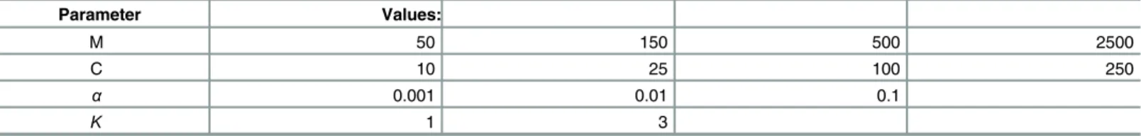
val-ues forM,α,KandCgiven inTable 2. For each parameter set, we create 10 independent
realizations.
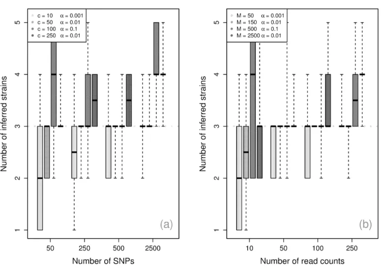
Number of components. Fig 3shows the algorithm’s performance for inferring the num-ber of components becomes more accurate with the numnum-ber of SNPs and the numnum-ber of reads, with 50 SNPs and 25 read counts sufficient to reliably recover the simulated values. With more SNPs, the requirement on read counts can be reduced to 10 with similar performance.
Condi-tional uponα, the simulations indicate that the number of SNPs is the largest determinant of
performance, and the sum of the read counts playing an important supporting role. Inference
of the number of strains is generally strong at low panmixture levels (smallαvalues), but is
noticeably more conservative forα= 0.1.
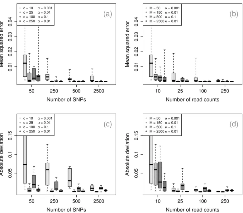
Parameters. Fig 4shows similar performance for inference of the strain proportions,W,
and panmixture coefficient,α. ForW, we report the mean squared deviation. Forα, we report
the absolute normalized deviation to account for relative difference from the true value. For both parameters, we observe that the number of SNPs is the strongest determinant of accuracy,
withM= 150 ensuring moderately strong performance. Again, highαmoderately decreases
the quality of inference for the strain proportions.
Table 2. Table of simulated parameter values.Cis the number of read counts whileM,Kandαare as inTable 1.
Parameter Values:
M 50 150 500 2500
C 10 25 100 250
α 0.001 0.01 0.1
K 1 3
Laboratory artificial mixtures
We apply the algorithm to 18 artificial laboratory mixtures. These artificial samples were gen-erated by taking stock of two standard Pf lines, DD2 and 7G8, and adding them together in the
fixed proportions given inS1 Table, and completing then Illumina sequencing and
variant-call-ing with usvariant-call-ing the same protocols as [27]. Samples had a median of 65 reads for the variants
considered here. Complete sequencing protocols and laboratory methods detailed in [35] (data
available at European Nucleotide Archive). Both strains have high-confidence reference sequences. We subsample 2000 SNPs from the 23,109 SNPs available for comparison based on
non-reference WSAF. The results inS1 Tableshow very strong agreement between the
labora-tory and inferred mixtures. The inferredαfor all samples was less than 0.001 and had Bayes
factor for non-zeroαas less than 1, indicating that the samples have little unexplained mixture
observed relative to the field samples.
Clinical samples from northern Ghana
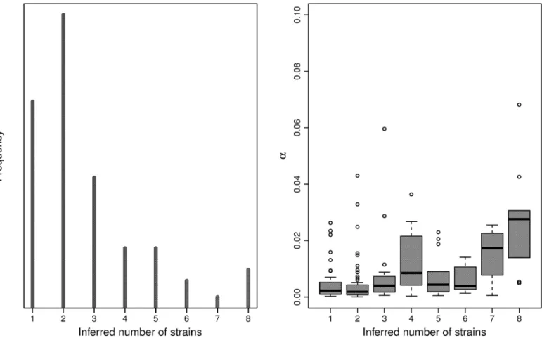
Applying the algorithm to the 168 high-quality samples from KND, we observe numbers of
strains ranging from 1 to 7, withαfalling between 0 and 0.14, and a moderate correlation
Fig 3. Component inference.Maximum a posteriori(MAP) inferred number of components by number of read counts across 10 simulations, with dotted line at the true number of components.
betweenKandα(Fig 5). The largest subset of samples were unmixed, withK= 1 andα<0.01,
though the majority of samples exhibit low but noticeable levels of admixture, withK= 2, 3, 4
and 0.01α0.03. A small number of samples exhibit complex mixtures, withK>4 andα
typically greater than 0.02. These samples also exhibit the most variance in the posterior
esti-mate ofK, frequently ranging from 3 to 8. To examine the necessity of the panmixia model to
capture unexplained variation in the field samples, we calculate a Bayes factor for each sample
under the two models,M0:α= 0 andM1:α6¼0. Since this is a single parameter, we employ the
Savage-Dickey ratio calculation as in [43]. We find that 78 samples give factors larger than 10,
indicating strong evidence forM1, and 9 samples give factors larger than 100, indicating
over-whelming evidence forM1.
Fig 4. Performance for parameter inference.Upper row: mean squared deviation for strain frequencies by number of read counts (left) and by number of SNPs (right). Lower row: absolute normalized deviation for panmixia coefficient by number of read counts (left) and by number of SNPs.
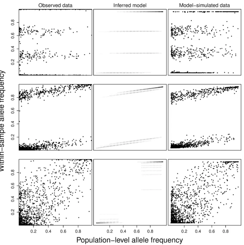
To visually inspect the quality of the results, we generate figures for each of the samples showing the observed WSAF and PLAF data, the inferred model structure, and data simulated under the inferred model following the observed PLAF. We show examples of these plots for
three typical samples inFig 6. Nearly all samples (158/168), across all different mixture
pat-terns, show strong visual correspondence between the observed and model-simulated data. Samples where PCR amplification was used (9 samples) exhibit no unusual features other than
low values forαrelative to the remaining samples. We also observe a strong correlation
between the inferred number of components and an estimate for the inbreeding coefficient for
each sample (Fig 7) [29]. These results are consistent with the high rate of MOI previously
observed in Ghanaian clinicial samples [24,44,45].
Discussion
In this work we show how to infer strain mixture within Pf isolates using WGS with two improvements over previous efforts: an additional model for unexplained variation based on a panmixia and a reversible jump implementation that accounts for uncertainty in the underly-ing number of strains. Simulations show that the model can perform accurate inference (MSE
<0.05 for strain proportions) with as few as 50 SNPs and 10 read counts per SNP. Simulations
with more than 100 SNPs or at least 25 read counts give highly accurate results (MSE<0.02).
In artificial laboratory mixtures the model provides excellent agreement with baseline mixture.
Fig 5. Ghanian sample summary.The frequency of inferred number of strains per sample (left) and and the panmixia coefficient by number of strains (right). MAP estimates used.
Fig 6. Examples of real and model-simulated data.For three samples (rows), we present the observed data WSAF plotted against the PLAF (first column), a diagram of the inferred model indicating the bands, proportions, and panmixia coefficient (second column), and data simulated under the inferred model. Panmixia coefficient and strain proportions are the MAP values. In the second column, the model’s PLAF-varying mixture densities are shown in grey scale, with black equal to one.
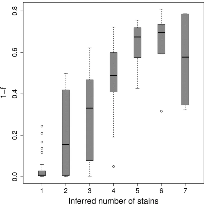
Fig 7. Number of strains by F-statistic.Boxplot of the inbreeding coefficient (1−Fis) for each sample grouped by the MAP number of inferred strains.
In field samples the model provides strong agreement with observed data and evidence based on Bayes factors indicates that some unexplained variation is present in a significant fraction of samples.
While the method works efficiently in practice, a number of possible improvements could strengthen its statistical performance. Most immediately, creating a full Bayesian approach
rather than the parallelizing implementation here—while likely not improving the parametric
inference for individual samples—would provide the full posterior distribution across all
sam-ples. The panmixia model is one of several possible approaches to dealing with additional within-sample variation that rigorous model comparison could reveal. The model also does
not perform haplotype phasing to resolve the sequence of the underlying strains [46–48]. The
analysis here suggests that a method for estimating haplotypes would be straight-forward for
some samples but difficult for others (say, whenαis greater than 0.05). Researchers may be
particularly interested in whether, in these phased samples, particular stretches of the genome appear more or less frequently in the dominant strains than others, indicating structures of immunological or environmental selection. This is a natural avenue for statistical methods development.
The model makes a number of simplifying assumptions that may be violated in practice. The model presumes that SNPs are unlinked and consequently independent for the purpose of calculating the likelihood. Given the high recombination rate of Pf this assumption may hold
for the majority of pairs of SNPs, but neglects correlations that appear locally (*10 kB).
How-ever, we expect that this independence assumption serves to moderately weaken the inferential power of the model rather than cause any type of bias since it effectively fails to include possibly
informative data. More problematic is the model’s implicit assumption of limited population
structure. In the case of the KND samples, and perhaps in much of west Africa, this assumption
appears supported [27,49]. In other contexts, specifically southeast Asia, recent population
bottlenecks and selection suggest that this assumption will be violated [50]. The consequences
on this model inference are unknown but may be partially resolved with appropriate simula-tion studies.
The model will work with any technology capable of typing multiple variants and where the measurement of the fraction of non-reference variants is unbiased. It was developed for WGS data but is not specific to the sequencing employed and should work similarly for Illumina, 454 and Pacific Bioscience read technologies. As noted in the results, we observe that the small number of field samples where PCR amplification was used did not appear unusual other than
exhibiting relatively lowαvalues. This is could be due to preferential amplification of the
dom-inant strains, suggesting that PCR-based approaches may obscure some aspects of natural infections. This model is not appropriate for data from RFLP assays or DNA microarrays with-out substantial modification.
In principle, the model can be explicitly tested against experimental mixtures more complex than those presented above. Laboratory facilities with the capacity to store many field strains
(>100) could generate artificial samples in an experimental analog of our simulation
proce-dure. Starting withNunmixed strains at equal dilution, they could create mixtures by first
fix-ing the required sequencfix-ing volume asη, and the desired parameters for panmixia (α), number
of component strains (K), and their mixture parameters,W. For thefinite mixture component,
they would then combine volumes ofZWfrom theKstrains. For the panmixture component,
they would thenfix some large number but experimentally feasible number of strains (say 50)
and randomly sample from all of them a volume ofη/50. Combining these into afinal sample
and applying WGS sequencing, will yield data that we hypothesize will closely follow the
inte-grated model outlined above, withνcapturing the experimental variation. Naturally, consistent
possibility of a more minimal description. These results could be further compared against
other next-generation technologies—such as single-cell sequencing—that have been deployed
to understand Pf clinical mixtures [51].
The model presents an important new tool for interrogating the biology of clinical Pf infec-tions. The ability to measure the structure of strain mixture connects to many aspects of Pf epi-demiology including seasonality, transmission intensity, outcrossing, and rates of gene flow. It also presents a means for clarifying the poorly detailed structure of intra-host infection
dynam-ics, such as strain selection or density-dependent selection [52], by resolving how the model
parameters change within the course of an infection or in response to drug intervention. This approach can serve as a means for researchers to empirically resolve these hypotheses.
Supporting Information
S1 Table. Table of output values from algorithm applied to artificial laboratory mixture data.
(PDF)
S1 Text. Accession numbers for raw data.
(PDF)
S1 Fig. Cut-off for low-quality samples.Number of missing SNPs for each sample in ascend-ing order (black dots) with the threshold used for cleanascend-ing (dotted blue line).
(PDF)
S2 Fig. Population structure of samples. Principal components (1–2, 1–3, 2–3) for samples and neighbor-joining tree of pairwise distance among samples both indicate limited popu-lation structure.
(PDF)
Acknowledgments
We thank Ana Lagunez for careful editing of the manuscript.
Author Contributions
Wrote the paper: JDO ZI LAE JW. Designed and implemented the study: JDO. Commented on the study design: ZI LAE. Generated artificial mixture data: JW. Performed all computational experiments: JDO. Performed data analysis: JDO. Commented on the analysis: ZI. Contributed all of the clinical data: LAE. Wrote and implemented the analysis tools: JDO. Commented on the development of the analysis tools: ZI.
References
1. Hay SI, Guerra CA, Gething PW, Patil AP, Tatem AJ, Noor AM, et al. A world malaria map:Plasmodium falciparumendemicity in 2007. PLoS Medicine. 2009; 6(3):e1000048. doi:10.1371/journal.pmed. 1000048PMID:19323591
2. Snow RW, Guerra CA, Noor AM, Myint HY, Hay SI. The global distribution of clinical episodes of Plas-modium falciparummalaria. Nature. 2005; 434(7030):214–217. doi:10.1038/nature03342PMID: 15759000
3. World Health Organization. World malaria report 2008. World Health Organization; 2008.
4. Wootton JC, Feng X, Ferdig MT, Cooper RA, Mu J, Baruch DI, et al. Genetic diversity and chloroquine selective sweeps inPlasmodium falciparum. Nature. 2002; 418(6895):320–323. doi:10.1038/ nature00813PMID:12124623
6. Payne D. Spread of chloroquine resistance inPlasmodium falciparum. Parasitology Today. 1987; 3 (8):241–246. doi:10.1016/0169-4758(87)90147-5PMID:15462966
7. Sidhu ABS, Verdier-Pinard D, Fidock DA. Chloroquine resistance inPlasmodium falciparummalaria parasites conferred by pfcrt mutations. Science. 2002; 298(5591):210–213. doi:10.1126/science. 1074045PMID:12364805
8. Roper C, Pearce R, Nair S, Sharp B, Nosten F, Anderson T. Intercontinental spread of pyrimethamine-resistant malaria. Science. 2004; 305(5687):1124–1124. doi:10.1126/science.1098876PMID: 15326348
9. Wilson R, McGregor I, Williams K, Hall P, Bartholomew R. Antigens associated withPlasmodium falcip-aruminfections in man. The Lancet. 1969; 294(7613):201–205. doi:10.1016/S0140-6736(69)91437-8 10. McGregor I. Immunology of malarial infection and its possible consequences. British Medical Bulletin.
1972; 28(1):22–27. PMID:4118010
11. Jamjoom GA. Dark-field microscopy for detection of malaria in unstained blood films. Journal of Clinical Microbiology. 1983; 17(5):717–721. PMID:6863496
12. Conway D, Greenwood B, McBride J. The epidemiology of multiple-clonePlasmodium falciparum
infections in Gambian patients. Parasitology. 1991; 103(Pt 1):1–6. doi:10.1017/S0031182000059217 PMID:1682870
13. Auburn S, Campino S, Miotto O, Djimde AA, Zongo I, Manske M, et al. Characterization of within-host
Plasmodium falciparumdiversity using next-generation sequence data. PloS one. 2012; 7(2):e32891. doi:10.1371/journal.pone.0032891PMID:22393456
14. Müller D, Charlwood J, Felger I, Ferreira C, Do Rosario V, Smith T. Prospective risk of morbidity in rela-tion to multiplicity of infecrela-tion withPlasmodium falciparumin São Tomé. Acta tropica. 2001; 78(2):155–
162. doi:10.1016/S0001-706X(01)00067-5PMID:11230825
15. Henning L, Schellenberg D, Smith T, Henning D, Alonso P, Tanner M, et al. A prospective study of Plas-modium falciparummultiplicity of infection and morbidity in Tanzanian children. Transactions of the Royal Society of Tropical Medicine and Hygiene. 2004; 98(12):687–694. doi:10.1016/j.trstmh.2004.03. 010PMID:15485698
16. Smith T, Beck HP, Kitua A, Mwankusye S, Felger I, Fraser-Hurt N, et al. 4. Age dependence of the mul-tiplicity ofPlasmodium falciparuminfections and of other malariological indices in an area of high endemicity. Transactions of the Royal Society of Tropical Medicine and Hygiene. 1999; 93(Supplement 1):15–20. doi:10.1016/S0035-9203(99)90322-XPMID:10450421
17. Färnert A, Rooth I, SvenssonÅ, Snounou G, Björkman A. Complexity ofPlasmodium falciparum infec-tions is consistent over time and protects against clinical disease in Tanzanian children. Journal of infectious diseases. 1999; 179(4):989–995. doi:10.1086/314652PMID:10068596
18. Stirnadel HA, Felger I, Smith T, Tanner M, Beck HP, et al. Malaria infection and morbidity in infants in relation to genetic polymorphisms in Tanzania. Tropical Medicine & International Health. 1999; 4 (3):187–193. doi:10.1046/j.1365-3156.1999.43381.x
19. Beck S, Mockenhaupt FP, Bienzle U, Eggelte TA, Thompson W, Stark K. Multiplicity ofPlasmodium fal-ciparuminfection in pregnancy. The American Journal of Tropical Medicine and Hygiene. 2001; 65 (5):631–636. PMID:11716126
20. Beck HP, Felger I, Vounatsou P, Hirt R, Tanner M, Alonso P, et al. 8. Effect of iron supplementation and malaria prophylaxis in infants onPlasmodium falciparumgenotypes and multiplicity of infection. Trans-actions of the Royal Society of Tropical Medicine and Hygiene. 1999; 93(Supplement 1):41–45. doi:10. 1016/S0035-9203(99)90326-7PMID:10450425
21. Smith T, Felger I, Fraser-Hurt N, Beck HP. 10. Effect of insecticide-treated bed nets on the dynamics of multiplePlasmodium falciparuminfections. Transactions of the Royal Society of Tropical Medicine and Hygiene. 1999; 93(Supplement 1):53–57. doi:10.1016/S0035-9203(99)90328-0PMID:10450427 22. Paganotti GM, Babiker HA, Modiano D, Sirima BS, Verra F, Konate A, et al. Genetic complexity of
Plas-modium falciparumin two ethnic groups of Burkina Faso with marked differences in susceptibility to malaria. The American Journal of Tropical Medicine and Hygiene. 2004; 71(2):173–178. PMID: 15306706
23. Mayengue PI, Luty AJ, Rogier C, Baragatti M, Kremsner PG, Ntoumi F. The multiplicity ofPlasmodium falciparuminfections is associated with acquired immunity to asexual blood stage antigens. Microbes and Infection. 2009; 11(1):108–114. doi:10.1016/j.micinf.2008.10.012PMID:19028595
25. Atroosh WM, Al-Mekhlafi HM, Mahdy MA, Saif-Ali R, Al-Mekhlafi AM, Surin J. Genetic diversity of Plas-modium falciparum isolates from Pahang, Malaysia based on MSP-1 and MSP-2 genes. Parasit Vec-tors. 2011; 4(4):233. doi:10.1186/1756-3305-4-233PMID:22166488
26. Joshi H, Valecha N, Verma A, Kaul A, Mallick PK, Shalini S, et al. Genetic structure of Plasmodium fal-ciparum field isolates in eastern and north-eastern India. Malar J. 2007; 6(60):10–1186.
27. Manske M, Miotto O, Campino S, Auburn S, Almagro-Garcia J, Maslen G, et al. Analysis of Plasmodium falciparum diversity in natural infections by deep sequencing. Nature. 2012; 487(7407):375–379. doi: 10.1038/nature11174PMID:22722859
28. Auburn S, Campino S, Clark TG, Djimde AA, Zongo I, Pinches R, et al. An effective method to purify
Plasmodium falciparumDNA directly from clinical blood samples for whole genome high-throughput sequencing. PLoS ONE. 2011; 6(7):e22213. doi:10.1371/journal.pone.0022213PMID:21789235 29. O’Brien J, Li R, Amenga-Etego L. Approaches to estimating inbreeding coefficients in clinical isolates
ofPlasmodium falciparumfrom genomic sequence data. bioRxiv. 2015;p. e021519.
30. Weir BS, Cockerham CC. Estimating F-statistics for the analysis of population structure. Evolution. 1984;p. 1358–1370. doi:10.2307/2408641
31. Hill WG, Babiker HA. Estimation of numbers of malaria clones in blood samples. Proceedings of the Royal Society of London Series B: Biological Sciences. 1995; 262(1365):249–257. doi:10.1098/rspb. 1995.0203PMID:8587883
32. Guerra CA, Gikandi PW, Tatem AJ, Noor AM, Smith DL, Hay SI, et al. The limits and intensity of Plas-modium falciparumtransmission: implications for malaria control and elimination worldwide. PLoS medicine. 2008; 5(2):e38. doi:10.1371/journal.pmed.0050038PMID:18303939
33. Balding DJ. Likelihood-based inference for genetic correlation coefficients. Theoretical population biol-ogy. 2003; 63(3):221–230. doi:10.1016/S0040-5809(03)00007-8PMID:12689793
34. Galinsky K, Valim C, Salmier A, de Thoisy B, Musset L, Legrand E, et al. COIL: a methodology for eval-uating malarial complexity of infection using likelihood from single nucleotide polymorphism data. Malaria Journal. 2015; 14(1):4. doi:10.1186/1475-2875-14-4PMID:25599890
35. Wendler J. Accessing complex genomic variation in Plasmodium falciparum natural infection. Doctoral dissertation, University of Oxford. 2015;.
36. Gardner MJ, Hall N, Fung E, White O, Berriman M, Hyman RW, et al. Genome sequence of the human malaria parasitePlasmodium falciparum. Nature. 2002; 419(6906):498–511. doi:10.1038/nature01097 PMID:12368864
37. Redner RA, Walker HF. Mixture densities, maximum likelihood and the EM algorithm. SIAM review. 1984; 26(2):195–239. doi:10.1137/1026034
38. McLachlan G, Peel D. Finite mixture models. John Wiley & Sons; 2004.
39. Gelman A, Carlin JB, Stern HS, Dunson DB, Vehtari A, Rubin DB. Bayesian data analysis. CRC press; 2013.
40. Gilks WR. Markov chain Monte Carlo. Wiley Online Library; 2005.
41. Geyer CJ. Practical Markov chain Monte Carlo. Statistical Science. 1992;p. 473–483. doi:10.1214/ss/ 1177011137
42. Scholz F. Maximum likelihood estimation. Encyclopedia of statistical sciences. 1985;.
43. Suchard MA, Weiss RE, Sinsheimer JS. Bayesian selection of continuous-time Markov chain evolution-ary models. Molecular Biology and Evolution. 2001; 18(6):1001–1013. doi:10.1093/oxfordjournals. molbev.a003872PMID:11371589
44. Owusu-Agyei S, Asante KP, Adjuik M, Adjei G, Awini E, Adams M, et al. Epidemiology of malaria in the forest-savanna transitional zone of Ghana. Malar J. 2009; 8(1):220. doi:10.1186/1475-2875-8-220 PMID:19785766
45. Felger I, Maire M, Bretscher MT, Falk N, Tiaden A, Sama W, et al. The dynamics of natural Plasmodium falciparum infections. PLoS One. 2012; 7(9):e45542. doi:10.1371/journal.pone.0045542PMID: 23029082
46. Stephens M, Smith NJ, Donnelly P. A new statistical method for haplotype reconstruction from popula-tion data. The American Journal of Human Genetics. 2001; 68(4):978–989. doi:10.1086/319501PMID: 11254454
47. Howie B, Fuchsberger C, Stephens M, Marchini J, Abecasis GR. Fast and accurate genotype imputa-tion in genome-wide associaimputa-tion studies through pre-phasing. Nature Genetics. 2012; 44(8):955–959. doi:10.1038/ng.2354PMID:22820512
49. Anderson TJ, Haubold B, Williams JT, Estrada-Franco JG, Richardson L, Mollinedo R, et al. Microsatel-lite markers reveal a spectrum of population structures in the malaria parasitePlasmodium falciparum. Molecular Biology and Evolution. 2000; 17(10):1467–1482. doi:10.1093/oxfordjournals.molbev. a026247PMID:11018154
50. Miotto O, Almagro-Garcia J, Manske M, MacInnis B, Campino S, Rockett KA, et al. Multiple populations of artemisinin-resistantPlasmodium falciparumin Cambodia. Nature Genetics. 2013; 45(6):648–655. doi:10.1038/ng.2624PMID:23624527
51. Nair S, Nkhoma SC, Serre D, Zimmerman PA, Gorena K, Daniel BJ, et al. Single-cell genomics for dis-section of complex malaria infections. Genome research. 2014; 24(6):1028–1038. doi:10.1101/gr. 168286.113PMID:24812326