www.scielo.br/rbg
EVALUATION OF THE TRANSIENT ELECTROMAGNETIC GEOPHYSICAL METHOD
FOR STRATIGRAPHIC MAPPING AND HYDROGEOLOGICAL DELINEATION
IN CAMPOS BASIN, BRAZIL
Antonio Abel Gonz´alez Carrasquilla
1and Emin Ulugergerli
2Recebido em 21 junho, 2006 / Aceito em 14 setembro, 2006 Received on June 21, 2006 / Accepted on September 14, 2006
ABSTRACT.The applicability of the Transient Electromagnetic (TEM) geophysical method for stratigraphic mapping and hydrogeological delineation has been tested in terrestrial part of the Campos Basin in Brazil. The study area is located within the fluvial plain of Para´ıba do Sul River, at the W edge of the continental portion of the Basin, geologically consisting of Tertiary and Quaternary sediments and a gneissic basement. Around 32 central loop TEM soundings were made with 10 or 20 m-sided transmitter loops, to map the conductive and/or resistive zones in the subsurface, which were correlated with lithology from a drilled borehole in the test area, whose location was indicated by the present study. In general, the one-dimensional (1D) models constructed for the TEM field data suggest a 3-layer resistivity structure characterized by a resistor-conductor-resistor pattern. The shallow section of 100-500 ohm.m and 50 m average thickness is interpreted as correlating with clay and shaly sand formations. The intermediate layer, with thickness around 20 m and resistivity less than 10 ohm.m, corresponds to clay. The basal resistor of 10-100 ohm.m at depths of more than 60 m at most sites is interpreted as the combined signature of the basal conglomerates, shaly sands and crystalline basement. Comparison with borehole data shows that the zone corresponding to the conductive geoelectrical units contains many thin layers of clay and sand that cannot be individually resolved by the TEM data and that there are no thick aquifers in the investigated area. In addition to that the shaly sand sediments have iron rich clays, which pollute groundwater, deeper resistive layers formed by conglomerates are considered the main aquifers of this area.
Keywords: transient electromagnetic, inverse one-dimensional interpretation, Campos Basin, stratigraphic mapping, hydrogeological delineation.
RESUMO.A aplicabilidade do m´etodo geof´ısico Transiente Eletromagn´etico (TEM) foi testada na parte terrestre da Bacia de Campos, Sudeste do Brasil, no mapea-mento estratigr´afico e no delineamapea-mento hidrogeol´ogico. A ´area do estudo, situada na borda W da porc¸˜ao continental da bacia e dentro da plan´ıcie fluvial do Rio Para´ıba do Sul, consiste geologicamente de sedimentos Terci´arios e Quatern´arios sobre um embasamento gn´aissico. Os trabalhos de campos consistiram de 32 sondagens com o arranjoloopcentral, com uma extens˜ao lateral 10 ou 20 m. O objetivo central do levantamento foi o de mapear as zonas condutoras e/ou resistivas em subsuperf´ıcie, as quais foram correlacionadas com a litologia de um poc¸o perfurado na ´area estudada, cuja localizac¸˜ao foi indicada a partir deste estudo. Em geral, os modelos unidimensionais (1D) resultantes da interpretac¸˜ao dos dados de campo sugerem uma estrutura de trˆes camadas, a qual ´e caracterizada por uma intercalac¸˜ao resistor-condutor-resistor. A sec¸˜ao rasa, de 100-500m de resistividade e uma espessura m´edia de 50 m, ´e interpretada como estando constitu´ıda por formac¸˜oes areno-argilosas. A camada intermedi´aria, com espessura em torno de 20 m e resistividade menor que 10m, corresponde `a argila. O resistor basal, de 10-100m de resistividade e em profundidades maiores que 60 m, ´e interpretado, na maioria dos locais de medic¸˜ao, como uma combinac¸˜ao de conglomerados, formac¸˜oes areno-argilosas e embasamento cristalino. Por outro lado, a comparac¸˜ao com dados do poc¸o mostra que a camada condutora intermedi´aria cont´em muitas camadas finas de argila e de areia, as quais n˜ao podem ser resolvidas individualmente pelos dados experimentais. Al´em disso, como n˜ao existe um aq¨u´ıfero expressivo na ´area investigada e os sedimentos areno-argilosos s˜ao ricos do ferro, o que causa poluic¸˜ao na ´agua subterrˆanea, isto torna a camada conglomer´atica resistiva profunda como o principal aq¨u´ıfero desta ´area.
Palavras-chave: transiente eletromagn´etico, interpretac¸˜ao unidimensional inversa, Bacia de Campos, mapeamento estratigr´afico, delineamento hidrogeol´ogico.
1Laborat´orio de Engenharia e Explorac¸˜ao de Petr´oleo, Universidade Estadual do Norte Fluminense Darcy Ribeiro (LENEP/UENF), Rodovia Amaral Peixoto, Km 163, Av. Brennand s/n, 29925-310 Imboacica, Maca´e, RJ, Brasil. Tel. +55 (22) 2796-9700 – E-mail: [email protected]
334
TEM GEOPHYSICAL METHOD IN ON-SHORE CAMPOS BASININTRODUCTION
The surveyed area is located in Campos City, Northern of Rio de Janeiro State – Brazil, and it belongs to the terrestrial part of Cam-pos Basin, which has a total sedimentary portion of 30.000 km2
, with only 600 km2
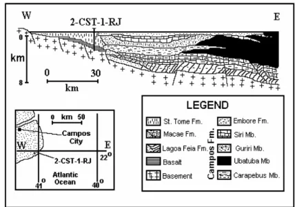
in the continental portion (Figure 1). This ba-sin is limited offshore by the Vit´oria Arc (N), Cabo Frio Arc (S) and by the ocean crust within the continental platform (E), while, on-shore, (W) it is bordered by a crystalline gneissic basement (DRM/PETROBRAS, 1997). In this terrestrial part, along of the W edge of the basin, S˜ao Tom´e Member grades for a thin red conti-nental alluvium section of Quaternary age in contact with the Ter-tiary sediments of the Barreiras Group, overlying Mesozoic volca-nic and Precambrian crystalline rocks (Figure 2). The sediments are deriving of gradation in the deposits of the deltaic system of the Para´ıba do Sul river (Figure 1), in which, are possible to iden-tify an intense integration of alluvium facies, swamp and lagoon sediments, lagoon evaporites and extensive beach lines, forming a geomorphology of coastal plain. On the other hand, the Barrei-ras Group, very common in the Brazilian coast, is constituted by fine argillaceous sands, gross siltstones, and conglomerates in-tercalate with argillaceous and bauxites layers (Figueiredo, 1985).
Figure 1– Location of survey area (modified from Carrasquilla et al., 1999).
Geophysical methods in Campos Basin were firstly used by PETROBRAS (Brazilian Oil Company), which performed terrestrial and marine gravity and seismic surveys. A year later, it was drilled the first well in S˜ao Tom´e Cape in 1959 (2-CST-1-RJ, Figure 2), which was perforated to obtain stratigraphic information, which did not reveal any presence of oil or gas, and, in this form, pro-voked the end of land prospecting works (Munis, 1993). This bo-rehole is located around of 25 km SE of the studied area (see small map in Figure 2) and it showed a succession of 1.960 m of Qua-ternary sediments (clay, sand, sandy-clay, clayey-sand and shale)
above 620 m of basalt flow, and then, a gneissic basement (Schal-ler, 1973). The Brazilian Geological Survey (CPRM), on the other hand, performed regional magnetic and gamma-spectometric sur-veys in Rio de Janeiro State, including Campos Basin (Mour˜ao, 1995). With the maps derived from this study, it was possible des-cribe the main geological trends that domain the region, which can be used as a guide in the detailed studies, as the objective of this paper. Furthermore, Fernandes et al. (1997) and Pavie (2004) performed several geophysical profiles, starting from th-ree different cities at the coast (S˜ao Tom´e Cape, S˜ao Jo˜ao da Barra e Barra do Furado) until crossing Campos City, using magnetotel-lurics (MT) and Long Off-Set Transient Electromagnetic (LOTEM) methods (Figures 1 and 2). These works were able to show the thickness of the sediments from the surface to the basement, be-sides a regional geological structure in a rift form with a SW-NE direction, which is coincident with the main structural outlines of the continental part of Campos Basin.
Transient Electromagnetic Method (TEM) has been success-fully applied to delineate stratified structures of geological inte-rest, as well as, in the prospecting of groundwater, geothermal bodies, sulfide ores, deep graphite conductors, etc. (Fitterman & Stewart, 1986), but had not been tested in Northern of Rio de Ja-neiro. Recently, this method has become into the most efficient technique to correct the static shift, which distorts the magneto-telluric soundings (Meju et al., 1993). In this work, we tested this geophysical technique in the specific geological conditions of on-shore Campos Basin, with the objective to map the stratigraphy of a small part of the basin, and, consequently, to delineate its hy-drogeologic characteristics. Thus, to supply water for the local needs, we looked for the thickness of the polluted layers and with the aim to take some precautions in the design and completion of the well, so that casing may be placed in order to prevent the natural contamination caused by mixing iron rich water coming from thin iron rich clays with potable water coming from deeper aquifer (conglomerate bands or fracture basement). This natural contamination is revealed an existing shallow well in the neigh-borhood of the surveyed area (30 m E of distance), which shows a water level around 5 m and produces polluted water (Carrasquilla et al., 1999).
To perform the survey using TEM method, one strong direct current is passed through a non grounded loop (Nabighian & Macnae, 1988). At timet = 0, this current is interrupted and
mea-Figure 2– Sedimentary package in Campos Basin (after Schaller, 1973).
sured in different times, which are related to different geological materials in the subsurface (Figure 4). Field procedure consists in performing several electromagnetic sounding along a profile, to show resistivity changes in distance and depth. Generally, the results can also be shown as soundings and its inverse one di-mensional (1D) interpretation (Figure 10), but, usually, they are presented in apparent resistivity pseudosection forms (Figures 8 and 9).
Figure 3– Current and primary magnetic field, induced electromotive force and secondary magnetic field in TEM method (modified from Nabighian & MacNae, 1988).
Figure 4– Subsurface induced current system (modified from Nabighian & MacNae, 1988).
In this survey, the used equipment measures the decay rate of the induction vertical magnetic component in nV/A m2
, and, after that in the way of a decay voltage, these measured values are transformed in apparent resistivity (ρa inm), as is shown by
the following equation (Fitterman & Stewart, 1986):
ρa= µ
4πt
b2A2I
5t V 2/3
, (1)
whereµis the magnetic permeability (1,2566×10⁻⁶m kg
C−2
),bis the square transmitter loop side (in m),Ais the effec-tive area of the receiver loop (area×number of coils), I is the electrical current in the transmitter loop (Amp),V is the transient voltage (Volt) andt, the time since the beginning of the transient (in sec).
For data processing, we used the TEMIXXL commercial pro-gram (INTERPEX, 1996), while for data interpretation we utilized a 1D algorithm, which utilized the dumped least square inversion algorithm (ridge regression) for horizontal layers, also incorpo-rated in TEMIXXL. In this algorithm the vector of parameters (−→P, 1D model of resistivities and thicknesses for each layer) and field observations (G, apparent resistivities) may be wrote as an ap-proximate linear expression relating changes in−→P to changes inG:
G=A−→P +ε , (2)
whereεis the fitting error, andAis the matrix sensitivity matrix, which it is defined as:
Ai j = ∂Gi ∂Pj
336
TEM GEOPHYSICAL METHOD IN ON-SHORE CAMPOS BASINwherei is the number of observations and j is the number of parameters.
IfAis overdetermined, the departures from linearityεis small and the initial guessPois close to the best-fitting vector of
para-meters−→P, we may obtain−→P =−→P −−→Povery simply from
the algorithm:
−→P =ATA−
1
ATG, (4)
where the superscriptsT and−1denote transpose and inverse,
respectively. Equation (4), which is known as least squares method, is obtained merely multiplied both sides of Equation (2) by the generalized inverse operator:
H=ATA −1
AT . (5)
Although Equation (4) is exceedingly fast when it converges, it is unfortunately highly unstable and usually diverges unless the data error is small and the initial guess is very accurate. In order to en-sure convergence from poor initial guesses, we generally sacrifice some speed and modify Equation (4) as follows:
−→P =ATA+k I−
1
ATG, (6)
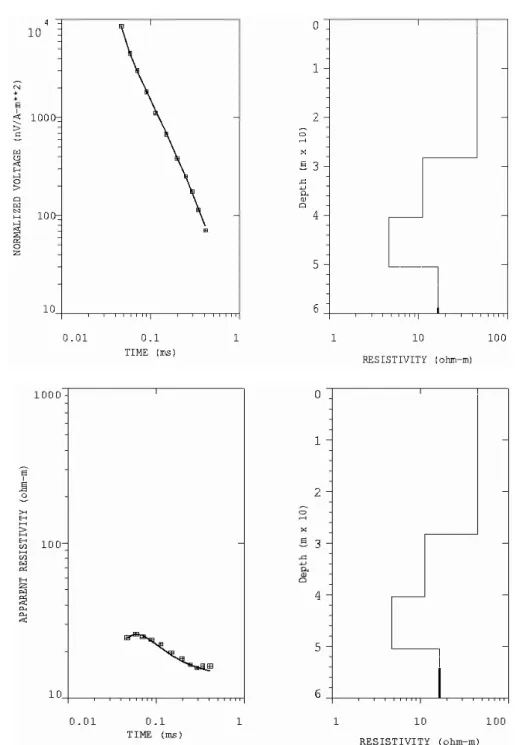
whereI is the identity matrix andk is some positive quantity. Ifkis very large, Equation (6) approaches the gradient method, which is slow but always converges. At the other extreme, ifkis very small approaches Equation (4), which is very fast but may diverge. The technique of altering the value ofkduring the pro-cess of inversion in order to ensure stable and fast convergence is known as dumped least squares or ridge regression (Rijo et al., 1977). An example of this kind of 1D inverse interpretation using this procedure is shown in Figure 10, corresponding to Soun-ding 2.
FIELD EXPERIMENTS
Measurements were made using the SIROTEM MK3 equipment, covering an area of 15.000 m2, approximately, performing 32 TEM
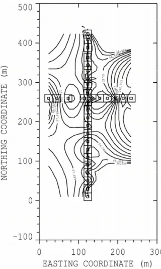
soundings, which were obtained using a central loop array with 10 and 20 m of loop side, depending on geometrical constraints at the site. The survey was developed in a whole day work through two cross-profiles: one in the E–W direction (10 soundings, cal-led Profile 1) and the other in the N–S direction (22 soundings, called Profile 2), where the center of each square corresponds to the center of the sounding.
RESULTS
The obtained data was plotted in the form of resistivity contour maps shown in Figures 5, 6 and 7. The Figure 5 shows the re-sistivity values obtained in earlier times (shallower depths). It is possible to observe high resistivity values in all area, and speci-ally, higher values in the W, NE and SE sectors. In the Figure 6, re-garding middle time (intermediate depths), we can see low values of resistivity, probably associated to the presence of conductive clays at this depth. In the Figure 7, related with later times (larger depths), we can observe intermediate resistivity values on W and SE of the prospected area, probably related with clay sediments mixture with sand, conglomerate or fractured basement.
Figure 5– Resistivity contour maps at early times.
Figure 6– Resistivity contour maps at middle times. Figure 7– Resistivity contour maps at late times.
we can observe a first layer with high resistivity values (up to
250m) and an average thickness of 30 m. The second layer
is a conductive one, with resistivity around10m and thickness
of 30 m. Below these two layers, it is possible to observe alter-nated conductive (10m) and resistive (50m) vertical bands.
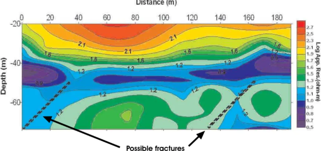
Initially, it was interpreted the resistive bands as fresh crystalline rock, the conductive ones as fractures within the basement, fil-led by groundwater and/or clay. After the drilling, we discovered that in these depths are locating a mixture of sand and conglome-rate layers with gneissic basement. Profile 2, on the other hand, shows the same resistive layer in the first meters of depth, with resitivities up to60m and 30 m of thickness (Figure 9). Below
this layer, it is possible to observe some conductive intervals with
10m of resistivity, but not in a continuous and clear pattern.
Below 60 m of depth, it is observed alternative resistive and con-ductive bands, also interpreted initially as fresh rock and fractures. The white band that appears at a distance of 150 m and at 70 m of
depth, it may be caused by the absence of signal in these depths. The difference between two sections (Figures 8 and 9) could be explained by a resistivity anisotropy.
According to the results and the interpreted data, it was de-cided to drill a borehole in the coordinate X = 20 m and
Y = 260m in Profile 1 (Figure 5), with the initial objective
una-338
TEM GEOPHYSICAL METHOD IN ON-SHORE CAMPOS BASINFigure 8– Apparent resistivities pseudosection of TEM Profile 1.
Figure 9– Apparent resistivities pseudosection of TEM Profile 2.
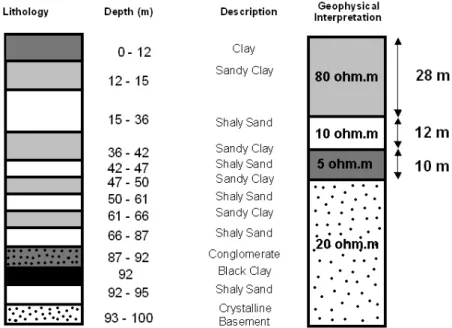
ble to differentiate thin layers, especially when they are conductive and resistive in alternate way. Thus, these two intermediate layers with resistivities of10m and5m and thicknesses of 12 m
and 10 m, respectively, can be interpreted as conductivity one, associated to clay formations. On the other hand, this method re-gistered the presence of a deep resistive geological formation that we interpreted, initially, as bedrock with fractures and fresh rock. Therefore, the drilled hole revealed that the deeper resistive geolo-gical formation as related to the presence of a combination of con-glomerate and crystalline rock. Thus, among of the geophysical methods, TEM was unable to identify thin layers and to eliminate the ambiguity in the identification of deeper geological formations. The integration of the geophysical interpretation and the ge-ological information allowed us to decide where to set casing, in this case, along shallows layers and the iron rich clayey conduc-tive layer (between 0 and 55 m), which was suppose to pollute the groundwater, and put an appropriated screen in the deep aqui-fer, and thus, to permit the flux of fresh water inside the well.
The well produced a flow rate of 20.000 lt/hr in the pumped test, which can be considered as reasonable. The chemical analysis of the produced groundwater in this well showed low concentrations of iron (100 ppm) but a high conductivity of 300 mS/m (related to salt concentration), which, in accord with HWO (Health World Organization) can be considered as potable water (EPA, 1990 a and b). These results show that using integrated geophysical and geological information from wells are much better than any crite-ria for stratigraphic mapping and hydrogeological delineation, as can be compared with the bad neighbor boreholes drilled in this area, which produces iron rich polluted groundwater.
CONCLUSIONS
Me-Figure 10– TEM Sounding 2 and its inverse 1D interpretation.
anwhile, the well drilled in the area, as suggested by the results of this study, revealed that the deep resistive layer was related to a conglomerate with lens of clay, that we previously interpreted as bedrock fractures. In spite of this ambiguity, the study was important to separate conductive and resistive layers, and, by the history of the area, freshwater can be only found in resistive layers related to porous sediments (sand or conglomerate) or in
340
TEM GEOPHYSICAL METHOD IN ON-SHORE CAMPOS BASINFigure 11– Well drilled besides TEM Sounding 2 and its inverse 1D interpretation.
ACKNOWLEDGEMENTS
This work was supported by grants from Brazilian Program to Support and Develop of Science and Technology (PADCT III) and Rio de Janeiro State Science Foundation (FAPERJ). We also ack-nowledge the Brazilian Research National Council (CNPq) for pro-viding research fellowship. One of the authors (E.U.) thanks Uni-versity of Ankara (Turkey) for providing support as a visiting re-searcher in ON/MCT. Finally, we thank Dr. Maxwell Meju from Lancaster University – UK for the revision of the text.
REFERENCES
CARRASQUILLA A, FONTES SL, LA TERRA EF & GERMANO CR. 1999. Estudo geof´ısico preliminar com os m´etodos TEM/FEM na Plan´ıcie Cos-teira Norte Fluminense. Proceedings, 6thInternational Congress of the Brazilian Geophysical Society, Rio de Janeiro, CD-ROM SBGf26.
DRM/PETROBRAS. 1997. Mapa Geol´ogico do Estado do Rio de Janeiro. Escala 1:400000.
EPA. 1990a. Ground Water. Volume I: Ground Water and Contamination. US Environmental Protection Agency, Office of Research and Develop-ment, Center for Environmental Research Information, Cincinnati, 144 p.
EPA. 1990b. Ground Water. Volume II: Methodology. US Environmen-tal Protection Agency, Office of Research and Development, Center for Environmental Research Information, Cincinnati, 141 p.
FERNANDES M, CARRASQUILLA A, FONTES S & RIBEIRO HJS. 1997. Primeiros resultados com o m´etodo geof´ısico magnetotel´urico no
es-tudo das feic¸˜oes geol´ogico estruturais da porc¸˜ao continental da Bacia de Campos. Proceedings, V Simp´osio de Geologia do Sudeste, Penedo – RJ, p. 365–367.
FIGUEIREDO AMF. 1985. Geologia das bacias brasileiras. In: VIRO EJ (Ed.). Avaliac¸˜ao de formac¸˜oes no Brasil. Schlumberger, Rio de Janeiro, I: 1–38.
FITTERMAN DV & STEWART MT. 1986. Transient electromagnetic soun-ding for groundwater. Geophysics, 51(4): 995–1005.
INTERPEX Ltd. 1996. Software Operation Manual TEMIXXL. Vol. I e II.
MEJU MA, FONTES SL & OLIVEIRA MFB. 1993. Joint TEM/AMT fe-asibility studies in Parna´ıba basin, Brazil: Geoelectrostratigraphy and groundwater resource evaluation in Piau´ı state. In: International Con-gress of the Brazilian Geophysical Society. Expanded Abstracts, Rio de Janeiro, SBGf, 3: 1373–8.
MOUR˜AO LMF. 1995. Base de Dados de Projetos Aerogeof´ısicos do Brasil (aero). Proceedings, 4thInternational Congress of the Brazilian Geophysical Society, Rio de Janeiro, 237–239.
MUNIS M. 1993. Aplicabilidade do m´etodo de Euler na interpretac¸˜ao de dados aeromagn´eticos da Bacia de Campos. Master Thesis, ON/MCT, Rio de Janeiro. 126 pp.
NABIGHIAN MN & MACNAE JC. 1988. Time domain electromagne-tic prospecting methods. In: NABIGHIAN MN (Ed.). Electromagneelectromagne-tic methods in applied geophysics. Vol. 2, Part A, Chapter 6, 427–520.
RIJO L, PELTON WH, FEITOSA EC & WRAD SH. 1977. Interpretation of apparent resistivity data from Apodi Valley, Rio Grande do Norte, Brazil. Geophysics, 42: 811–822.
SCHALLER H. 1973. Estratigrafia da Bacia de Campos. Anais do XXVII Congresso Brasileiro de Geologia, Aracaju, 3: 247–258.
NOTES ABOUT THE AUTHORS
Antonio Abel Gonz´alez Carrasquillais PhD in geophysics (Federal University of Par´a, Brazil), specialist in electromagnetic methods for natural resources prospec-ting, mainly groundwater and oil. Actually, he is Professor and Head of the Petroleum Engineering and Exploration Laboratory of the North Fluminense State University in Maca´e – RJ, Brazil.