Hydrodynamic study of a Lander Platform for Subsea Operations

UNIVERSIDADE DA BEIRA INTERIOR

Engenharia

Hydrodynamic Study of a Lander Platform for

Subsea Operations

(Versão final após defesa)

José Jerónimo da Silva Gonçalves

Dissertação para obtenção do Grau de Mestre em

Engenharia Aeronáutica

(Ciclo de estudos integrado)

Orientador: Prof. Doutor Miguel Ângelo Rodrigues Silvestre

Co-orientador: Engenheiro Tiago Correia Bartolomeu

Acknowledgments

To all those who have accompanied me on this long journey in search of knowledge and wisdom, I express my most sincere gratitude. From my childhood educators to my university professors, I am sincerely grateful for all that they have taught me.

Firstly, I would like to thank my supervisor at UBI (Universidade da Beira Interior), Professor Miguel Silvestre for the time spent helping me, for the knowledge he has given me and for being always present, without him this dissertation would not be possible. I am genuinely grateful to CEiiA (Center of Engineering and Product Development) for the opportunity they gave me and all the support and conditions provided.

I am particularly grateful to my supervisor at CEiiA, Tiago Bartolomeu. You have consistently supported me and raised my head on the most difficult days. Thanks not only for your help, but also for your advice and friendly word. I couldn’t have had a better mentor. Further, this gratitude also includes CEiiA’s team: Marcos Moreira, Miguel Machado and Oleh Tkachuk.

I could not forget those who in these last months worked alongside me. André, Mariana, and es-pecially, Daniel for the support and contagious positive energy they gave me. Moreover, thanks to all my friends who accompanied me and somehow contributed: Filipe, Jeremias, Juan, Tiago, Marcos, Pedro, Luis, António, Sílvia, José, Daniel, Maria, Jorge, Francisca, David, Martim, Inês, Filipa, Rui, Gonçalo, Gustavo, Monte, Francisco and Flávio.

Finally, I thank my family and my girlfriend for all the patience, courage and unconditional love they gave me. To my parents, Maria and Jerónimo, I am eternally grateful that they are always there, letting me follow my dreams even though it may sometimes be painful to get away from them. To my brothers, Fátima, Mara, Sara, Laura and Francisco, thank you for everything. And to my girlfriend, Maria João, nothing I can say will express what you’ve done for me these months. You’re the best!

Dedication

Resumo

O estudo da sismografia no fundo dos oceanos é de extrema importância para prevenção de tsunamis. Estima-se que cerca de 500000 sismos são detetados anualmente, sendo que na maio-ria dos casos o epicentro está localizado nos oceanos. Deste modo, a sua deteção precoce semaio-ria uma mais valia para evitar, quer perdas humanas, quer perdas materiais. Atualmente utilizam-se sismómetros no fundo dos oceanos (OBS) como instrumentos de deteção sísmica. O preço destes instrumentos influencia bastante a sua precisão, o que poderá fazer com que sejam de-tetados diferentes intervalos de frequência. Um dos problemas que estes aparelhos apresentam é o ruído gerado pelo escoamento. Ruído este que, dependendo da sua frequência pode cor-romper o sinal transmitido. Por isso, é crucial estudar, hidrodinamicamente, a geometria que menos ruído gera, a fim de evitar alarmes indesejados.

O presente trabalho tem como principal objetivo analisar, através do software OpenFOAM (Open-source Field Operation And Manipulation), o comportamento do escoamento em torno de um cilindro, de forma a poder identificar, filtrar e/ou eliminar as frequências indesejadas induzi-das pelo escoamento. A velocidade máxima considerada para este estudo é 0.08 [m/s], que ali-ada às características do fluido e da geometria que se pretende estudar, resultou num número de Reynolds de 80000. Para este estudo, foram utilizadas as equações de Unsteady Reynolds-Averaged Navier-Stokes (URANS) com o modelo de turbulência κ-ω Shear Stress Transport (SST).

Foram analisadas diferentes razões de aspeto do OBS para se compreender qual era a variação da frequência induzida pelo escoamento. Foi observado que a frequência induzida pela escoa-mento decresce com a diminuição da razão de aspeto da geometria. Em seguida, analisou-se a configuração conceptual utilizando a escala 1:1, da qual se obteve uma frequência máxima de 0.0057 [Hz]. Com o objetivo de minimizar o ruido gerado pelo escoamento, foram sugeridas duas geometrias alternativas: um cilindro com uma calota esférica no topo e um cilindro com três cintas espirais. No final, foi conseguido reduzir em 60% a frequência induzida pelo escoa-mento, com o cilindro com uma calota esférica no topo.

Com a modificação sugerida, é possivel obter resultados que não comprometem o correto fun-cionamento do sismógrafo. Na impossibilidade de eliminar por completo o ruído, pode ser de-senvolvido um filtro eletrónico de forma a que estas frequências indesejadas sejam identificadas e excluídas da amostra.

Palavras-chave

Sismómetros de fundo do oceano, OpenFOAM, frequência, Dinâmica de Fluidos Computacional (CFD), carenagem.

Abstract

The seismography study in the oceans is extremely important for tsunami prevention. It is es-timated that annually are detected over 500000 and, in most cases, the epicenter is at the ocean. Thus, its premature detection would be an asset to avoid both human and material losses. Nowadays, Ocean Bottom Seismometers (OBS) are used as instruments of seismic de-tection. The price of these instruments greatly influences their accuracy, which may cause different frequency ranges to be detected. One of the main issues of these instruments is the noise generated by the flow. This noise, depending on its frequency, can corrupt the signal transmitted. For this reason, it is crucial to study, hydrodynamically, the geometry that gener-ates less noise, in order to avoid undesired alarms.

This project has the objective of analysing, through OpenFOAM (Open-source Field Operation And Manipulation) software, the flow behavior around a cylinder, to identify, filter and/or elim-inate the undesired frequencies induced by the flow. The maximum velocity considered for this study is 0.08 [m/s], which combined to the flow characteristics and the geometry intended to study, resulted in a Reynolds number of 80000. For this study, the equations utilized were Un-steady Reynolds-Averaged Navier-Stokes (URANS) with the turbulence model κ-ω Shear Stress Transport (SST).

In order to understand which was the flow-induced frequency variation, different OBS aspect ratios were analysed. It was observed that the induced frequency would decrease with the reduction of the aspect ratio. Following this, it was analysed with a scale 1:1 the conceptual configuration, which the result indicated a maximum frequency of 0.0057 [Hz]. Therefore, in order to minimize the noise generated by the flow, two alternative geometries were suggested: a cylinder with a spherical hubcap and a cylinder with three helical strakes. In the end, it was possible to achieve a 60% reduction in the induced frequency, with the cylinder with a spherical hubcap configuration.

Along with the suggested modification, it is possible to obtain results that do not compromise the correct functioning of the seismograph. Failing to eliminate completely the noise, an electronic filter should be developed, so that these unwanted frequencies could be identified and excluded from the sample.

Keywords

Ocean Bottom Seismometer, OpenFOAM, frequency, Computational Fluids Dynamics (CFD), shell configuration.

Contents

1 Introduction 1

1.1 Motivation . . . 1

1.2 Purpose and Contribution . . . 2

1.3 Research and Objectives . . . 3

1.4 Thesis Outline . . . 3

2 Literature Review 5 2.1 Sea Technologies . . . 5

2.1.1 Deep-Sea Benthic Landers . . . 6

2.1.2 Ocean Bottom Seismometer - History, Main Applications and Design . . . . 8

2.2 Flow around Cylindrical Structures . . . 10

2.2.1 Flow Regime . . . 10

2.2.2 Vortex Shedding . . . 12

2.2.3 Horseshoe Vortex . . . 14

2.2.4 Drag and Lift Forces . . . 16

2.3 Computational Fluid Dynamics . . . 18

2.4 Governing Equations of Viscous Flow . . . 18

2.4.1 Mass Conservation . . . 19

2.4.2 Momentum Conservation . . . 20

2.4.3 Energy Conservation . . . 21

2.5 General Transport Equation . . . 21

2.6 Modeling Approaches for Turbulence . . . 22

2.7 Turbulence Models . . . 23 2.7.1 Standard κ-ε model . . . 24 2.7.2 Standard κ-ω model . . . . 24 2.7.3 SST κ-ω model . . . . 25 2.8 State-of-the-Art . . . 25 3 CFD Methodology 27 3.1 CFD workflow . . . 27 3.2 OpenFOAM . . . 28 3.2.1 Model Setup . . . 28

3.3 Numerical Validation Setup . . . 30

3.3.1 Geometry Validation and Flow Domain Definition . . . 31

3.3.2 Mesh Generation . . . 33

3.3.3 Physical Model Setup . . . 35

3.3.4 Boundary Conditions . . . 36

3.3.5 Temporal Discretization . . . 37

3.4 Simulation . . . 38

3.5 Mesh Independence Study . . . 39

4 Case Study: OBS Shell 41

4.1 OBS Shell Conceptual Design . . . 42

4.1.1 Results . . . 42

4.2 OBS Shell Geometries . . . 44

4.2.1 Results . . . 44 4.3 Discussion . . . 45 5 Conclusions 49 5.1 Difficulties . . . 49 5.2 Results . . . 50 5.3 Future Work . . . 51 bibliography 53 A 59 A.1 OpenFoam Files . . . 59

B 77 B.1 On the Fly Documents . . . 77

C 79 C.1 FFT Process . . . 79

D 81 D.1 Three dimensions views . . . 81

List of Figures

1.1 Continental platform extension [1]. . . 2

1.2 DUNE shell. . . 2

2.1 Deep-Sea Technologies - Underwater Vehicles. . . 6

2.2 Micro tripod open-frame landers. . . 7

2.3 Macro open-frame landers. . . 7

2.4 Z3000 lander, adapted from [2]. . . 8

2.5 TWERC lander, adapted from [3]. . . 8

2.6 Disposal of OBSs on a ship, adapted from [4]. . . 9

2.7 OBS deployment, launch and recovery phases, adapted from [5] [6]. . . 10

2.8 Sketch from Leonardo da Vinci’s notebooks [7]. . . 12

2.9 Formation of a tip vortex in the wing [8]. . . 12

2.10 Vortex shedding evolving into a vortex street [9]. . . 13

2.11 Mechanism of vortex shedding [10]. . . 13

2.12 Von Karman Vortex Street at increasing Reynolds number [11]. . . 14

2.13 Strouhal number for smooth circular cylinder, adapted from [10]. . . 15

2.14 Horseshoe vortex formation, adapted. . . 15

2.15 Lift and drag forces traces, adapted from [10]. . . 17

2.16 Reynolds number vs circular cylinder drag coefficient as obtained by several re-searchers, adapted from [12]. . . 17

2.17 Fluid element for conservation laws, adapted from [13]. . . 19

2.18 Stress components, adapted from [13]. . . 20

2.19 Prediction methods, adapted from [14]. . . 23

3.1 CFD work scheme [15]. . . 27

3.2 Case configuration. . . 29

3.3 Case configuration. . . 29

3.4 Case configuration. . . 30

3.5 Validation process. . . 31

3.6 Cylinder base refinement. . . 32

3.7 Control volume representation. . . 32

3.8 CastellatedMeshControls process, adapted from [16]. . . 34

3.9 Surface snapping, adapted from [16]. . . 34

3.10 Layer addition, adapted from [16]. . . 34

3.11 Mesh wireframe. . . 35

3.12 Boundary layer subdivision. . . 36

3.13 Numerical vs. physical domain of dependence, adapted from [17]. . . 37

3.14 Mesh convergence results. . . 39

3.15 Validation results. . . 40

4.1 Case study configuration. . . 41

4.2 OBS shell. . . 42

4.3 CL as a function of time of conceptual design. . . 43

4.5 Three dimensional flow around conceptual design. Close view of horseshoe vortex. 43

4.6 OBS shell geometries. . . 44

4.7 Relation of the mean streamlines and pressure contours on the plane Y = 0. . . . 45

4.8 Relation of the mean streamlines and pressure contours on the Z = 20%H from the bottom plane. . . 46

4.9 Relation of the mean streamlines and pressure contours on the Z = 50%H from the bottom plane. . . 47

B.1 Forcesgnuplot file structure. . . 77

B.2 Residuals file structure. . . 77

C.1 FFT. . . 79

C.2 FFT process. . . 80

D.1 Three dimensional flow around spherical cap. Close view of horseshoe vortex. . . 81

D.2 Three dimensional flow around cylinder with three helical strakes. Close view of horseshoe vortex. . . 81

List of Tables

2.1 Regimes of flow around a smooth, circular cylinder in steady current, adapted

from [10]. . . 11

3.1 Flow domain dimensions. . . 32

3.2 Simulation boundary conditions. . . 37

3.3 Meshing commands. . . 38

3.4 Initialization commands. . . 38

3.5 Simulation commands. . . 39

3.6 Mesh convergence results. . . 39

3.7 Authors’ references. . . 40

4.1 Mission requirement. . . 42

Acronyms List

ASV Autonomous Surface Vehicle AUV Autonomous Underwater Vehicle BOBO BOttom BOundary

CEiiA Center of Engineering and Product Development CFD Computational Fluid Dynamics

CFL Courant-Friedrichs-Lewyor DNS Direct Numerical Solution DOBO Deep Ocean Benthic Observatory

DoF Degrees of Freedom

EMEPC Estrutura de Missão para a Extensão da Plataforma Continental FFT Fast Fourier Transform

FVM Finite Volume Method IDL Instituto Dom Luiz

ISIT Intensified Silicon Intensifier Target LES Large Eddy Simulations

OBJ Wavefront Object

OBS Ocean Bottom Seismometer

OpenFOAM Open-source Field Operation And Manipulation RANS Reynolds Averaged Navier-Stokes

ROV Remotely Operated Vehicle SST Shear-Stress Transport STL Stereolithography

TWERC Tsunami Warning and Early Response system of Cyprus UBI Universidade da Beira Interior

URANS Unsteady Reynolds Averaged Navier-Stokes US United States

UUV Unmanned Underwater Vehicle V&V Verification and Validation

Nomenclature

∆y First layer thickness [m]

∇T Temperature gradient [K/s]

CD Mean drag coefficient [−]

D Mean drag [N ]

b

D Oscillating drag amplitude [N ] bL Oscillating lift amplitude [N ]

CD Drag coefficient [−]

CL Lift coefficient [−]

Co Courant number [−]

D Drag [N ]

d Diameter [m]

e Internal energy per unit mass [J/kg]

fv Vortex shedding frequency [Hz]

l Characteristic linear dimension [m]

H Cylinder height [m]

k Coefficient of thermal conductivity [W/(m.K)]

L Lift [N ]

nu Fluid kinematic viscosity in OpenFOAM [m2_/s]

nut Kinematic eddy viscosity in OpenFOAM [m2_/s]

p Pressure [P a] Re Reynolds number [−] SE Source of energy [−] SM Source factor [−] St Strouhal number [−] t Time [s]

Tv Vortex shedding period [s−1]

U Velocity [m/s]

w Vector of work associated with each control volume face [−]

y+ _{Non-dimensional distance to the wall [−]}

Greek Letters

κ Turbulent kinematic energy [m2_/s2_]

µ Absolute viscosity [kg/(m· s)]

ν Kinematic viscosity [m2_/s]

ω Specific dissipation rate [s−1]

ωv Vortex shedding frequency [rad/s]

ϕv Phase angle [rad]

ρ Density [kg/m3_]

τ Shear stress [N/m2_]

τw Wall shear stress [kg/(m· s)]

Chapter 1

Introduction

1.1

Motivation

Oceans are the blood and essence of planet Earth and all humankind. They flow 97% of the planet’s water and extend over three quarters of the planet. These are responsible for the pro-duction of more than half of the oxygen present in the atmosphere and absorb the most carbon dioxide. Oceans are a fundamental piece of the Man’s existence on Earth, even though over 80%of this vast underwater kingdom remains unexplored, unmapped and unobserved [18] [19].

It is estimated that around 500000 earthquakes are detected annually due to natural causes, it is in the oceans that most epicenters are located. Among which, the strongest can originate tsunamis, bringing huge catastrophes to mankind. The most recent and catastrophic case that Portugal has witnessed, was the Lisbon earthquake in 1755, followed by a tsunami that destroyed most of the city. So, in order to better understand this unknown area and improve human life, it is important to explore it as much as possible without jeopardizing marine biodiversity.

Over the past decades, underwater operations in deep sea have been increasingly a topic of interest in the marine community, in which vehicles such as ROVs (Remotely Operated Vehicles) or AUVs (Autonomous Underwater Vehicles) are often used as tools for current operations at full ocean depth. However, a support ship is always needed to carry out missions with these vehicles, which imply associated operational costs.

When long term operations are desired, lander platforms are the most economic suitable option. These stable platforms are, autonomous and unmanned, oceanography research instruments to be deployed independently on the seabed over extended periods [20]. Ocean Bottom Seismome-ter are a good example of these platforms and, it is a receiver for seismic signals that can be heard near the seabed [21]. The major challenge when developing this type of instrument is to minimize the interference of the currents occurring at these depths, with the focus to receive a clean signal by the lander [22].

Exploration of the ocean floor can bring both great business opportunities and new scientific discoveries. Therefore, it is of great interest to be able to obtain information about it at low cost. Thus, it is relevant to use lander platforms for this purpose.

The ”Continental Shelf Extension Mission Framework” (EMEPC) has worked since 2005, so that in May 2009 it delivered a proposal for the extension of the continental shelf as shown in Figure 1.1. Once accepted, Portugal will have a continental shelf of about 3900000 kilometers, where 97% will consist of ocean [1].

For this reason, it is of great importance for Portugal to improve the level of ocean floor re-search, either for the prevention of natural catastrophes or for scientific research. Therefore,

Figure 1.1: Continental platform extension [1].

the use of landers is a great choice given its low cost and the possibility of having long term missions.

1.2

Purpose and Contribution

The dissertation was a challenge proposed by CEiiA, together with partnerships with UBI and IDL (Instituto Dom Luiz). The work developed in the dissertation will be made in parallel with the current DUNE project.

Currently, a first version of the OBS is already established (Figure 1.2). In the first place, a hy-drodynamic analysis will be made to the current configuration. Afterwards, modifications will be suggested to improve hydrodynamically and reduce the noise induced by the flow.

Figure 1.2: DUNE shell.

As OBS is a recent technology, there are still many improvements available. One of which is the reduction of signal interference due to flow currents in the mission depths. The main purpose

of this thesis is to reduce this interference in the signal of the OBS.

In order to evaluate this signal noise, OpenFOAM software will be used to hydrodynamically analyse the OBS. The use of this software is intended to validate it for unsteady ocean floor flows. So, in the future, one can have greater flexibility, control and experience in similar analyses.

1.3

Research and Objectives

The main focus of the dissertation is to identify, reduce or eliminate the noise in the OBS signal, from the interference of currents in its geometry. Thereby, the dissertation author outlined his goals with those of CEiiA and its partners, where a set of objectives were established. Those objectives include:

• Code validation for unsteady analysis; • Hydrodynamic study of different geometries; • Most suitable configuration selection.

Since errors are associated to numerical simulations, validation is an essential step to have confidence in the results. Hereafter, different configurations can be analised to select the best one according to the results and customer requirements.

1.4

Thesis Outline

The dissertation is subdivided into 5 chapters in a logical way and easy to understand order. A short description of each chapter is given below:

Chapter 1 begins with the author’s motivation, the purpose and contribution of the dissertation, and finally its research and objectives.

Chapter 2 presents the literature review, where an introduction to aquatic landers is presented sand also about flow around cylindrical bodies, relevant theory, and experimental studies de-veloped by other authors.

Chapter 3 describes the implementation of the CFD methodology. At the end of the chapter a mesh independence study is described, as well as the validation of the code by comparison with similar studies.

In chapter 4 the case study is outlined, where requirements and assumptions made are de-scribed. The results of the different configurations are presented and compared.

Finally, in the last chapter, chapter 5, is resumed the conclusions, difficulties and also future work.

Chapter 2

Literature Review

This chapter covers the review of all the topics considered relevant to the case study in question, such as UUV’s (Unmanned Underwater Vehicle) history, evolution of OBSs and the influence of its design on its performance, as well as a theoretical introduction to all the principles used. In this chapter, some examples of other analyses carried out by other authors will be presented. To conclude, a theoretical introduction to the methods and models will be given.

2.1

Sea Technologies

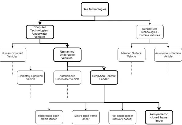
Once the dissertation is related to Ocean Bottom Seismometers, a detailed study of all sea technologies is not relevant. Still, in order to contextualize, it is important to understand the classification of OBS’s within the sea technologies. As can be seen in Figure 2.1, sea technolo-gies can be divided into two main categories: Deep Sea Technolotechnolo-gies, where there are manned and unmanned vehicles; and Surface Sea Technologies: which, like the previous one, can also be manned or unmanned.

Surface vehicles, as the name implies, are vehicles that operate at the surface of the oceans. Depending on the type of mission, they may have different configurations, power and accuracy. In recent years the technology of surface vehicles has passed through Autonomous Surface Vehi-cles (ASVs), since it has greater safety, autonomy and cost efficiency when compared to manned surface vehicles.

Hereinafter, a detailed description of Deep-Sea Benthic Landers will be given, once they are the vehicles of interest to this work. These can be subdivided according to the configuration of the vehicle. In the present work the focus goes to the axisymmetrical closed-frame lander, since the axisymmetric structure causes the flow to have the same behavior in the body regardless of the flow direction.

Depending on its mission, an OBS can be classified as [20]:

• Micro tripod open-frame landers; • Macro open-frame landers;

• Axisymmetric closed-frame lander; • Flat shape landers.

Figure 2.1: Deep-Sea Technologies - Underwater Vehicles.

2.1.1

Deep-Sea Benthic Landers

Deep-Sea Benthic Lander is a general term for an autonomous and unmanned oceanography research vehicle, which descends by free-fall to the ocean floor (without remote assistance), and operates independently on the ocean floor. The platforms have the purpose of collecting physical, biological and chemical variables over a predefined period of time. They operate in-dependently of the surface for periods of a few days, e.g. biological studies, up to a few years, e.g. physical oceanography studies. After completing its mission, the lander releases the ballast weight by an acoustic signal transmitted from the surface or by a pre-programmed device. The vehicle comes back to the surface by merit of its positive buoyancy [23] [24].

Reference [25] [26] present the different possible benthic landers configurations for their dif-ferent missions.

2.1.1.1 Micro tripod open-frame landers

Open frame tripod shape is the simplest lander configuration, which can be equipped with dif-ferent type of sensors, capturing images of deep sea creatures or analysing water quality.

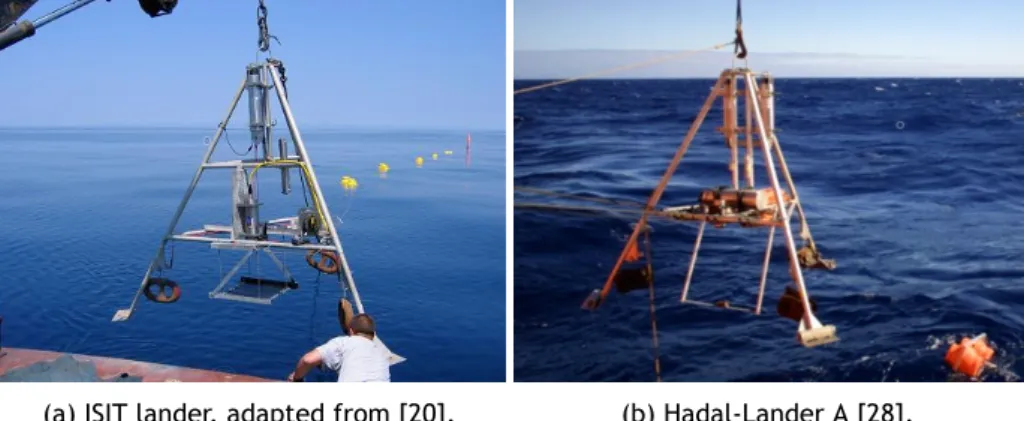
An example is the ISIT (Intensified Silicon Intensifier Target) lander, in which the purpose is to research stimulated and spontaneous bioluminescence emissions in the water column and ben-thic boundary layer to depths around 1000 [m], as well as fauna attracted to artificial food falls (Figure 2.2a) [27].

Another example is HADAL-Lander A (Figure 2.2b), known as Alfie, which is a free fall baited lander equipped with a high resolution video camera. This lander attracts the local fauna with the bait that is attached to it and then film the bait-attending fauna [28].

(a) ISIT lander, adapted from [20]. (b) Hadal-Lander A [28].

Figure 2.2: Micro tripod open-frame landers.

2.1.1.2 Macro open-frame landers

DOBO (Figure 2.3a), the Deep Ocean Benthic Observatory, lander was designed for larger pay-loads with the objective of observing the biological response due to deep-ocean physical pa-rameters. This lander was designed to operate for long periods, exceeding six months [29].

(a) DOBO lander. It is equipped with an acoustic Doppler current profiler (a), camera (b), battery (c), controller (d),

flash system (e), current meter (f),

adapted from [30]. (b) BOBO lander, adapted from [31].

Figure 2.3: Macro open-frame landers.

Netherlands Institute of Sea Research developed the BOBO (BOttom BOundary) Observatory (Fig-ure 2.3b), a four-meter tall lander for deep sea missions. Its struct(Fig-ure was designed to remain on the seabed for long periods, sometimes more than one year. This lander is adaptable to sev-eral configurations, it can measure near-bottom salinity, currents speeds, currents directions, temperature and it is equipped with cameras [32] [33].

2.1.1.3 Axisymmetric closed-frame lander

The mission purpose of each lander directly influences its mechanical shape. The open-frames landers are used in order to minimize the effects of currents from the sea and allow the water to flow through the instruments and sensors.

One of the advantages of the closed-frame configuration is its hydrodynamic shape that allows to reduce the noise caused by flow on the lander (Figure 2.4).

Figure 2.4: Z3000 lander, adapted from [2].

Z3000, developed by Magseis Fairfield is an axisymmetric lander [2]. It is autonomous, lightweight, easily released and retrieved, and it can go to depths down to 3000 [m]. Its principal mission is seismic analysis at the bottom of the ocean [2].

2.1.1.4 Flat shape landers

The last configuration to be described is the flat shape lander. Similarly to the previous one, the flat shape structure rests on the bottom with reduced exposed drag, and uses its hydrodynamic effect to act as free descending forces that anchor the lander.

Figure 2.5: TWERC lander, adapted from [3].

In Figure 2.5 one can see a flat shape system, called TWERK (Tsunami Warning and Early Response system of Cyprus), which is one of the offshore communications backbone. This lander belongs to the OceanWorks International’s seafloor network systems [34].

2.1.2

Ocean Bottom Seismometer - History, Main Applications and Design

Ocean Bottom Seismometer is traced back to the 30’s of the twentieth century. The first instru-ments were employed in military studies, but were abandoned when new procedures concerning near-surface sources and receivers were implemented. During the late 1950’s and early 1960’s, the United States (US) government has sparked a new life for OBS technology. The main purpose of the seismometers was to detect and identify clandestine nuclear explosions [35].

The ”Vela Uniform project” was one of the programs that made the most advances in OBS technology, requiring a uniform distribution of monitoring station around the planet, which conducted to the need for ocean seismic stations. Since then, the use of OBS’s for passive earthquake recording or active experiments has become very common for offshore scientific purpose, as well as gas and oil reservoirs research, and tsunami forecast [36].

Nowadays, OBSs are developed with different shapes and sizes depending on their mission: from short-period instruments for active source experiments, to large OBSs operating independently for one year or more. Technology has evolved since the release of the first OBS, but the prin-ciple of the system remains the same. It is a platform equipped with one or more sensors, and a disposable compartment, where the ballast weight is placed, that descends and lands on the ocean floor to record autonomously man-made or natural seismic signals. Completed the mis-sion time, or after receiving an acoustic signal, the disposable compartment is released and the OBS ascends to the ocean surface using its positive buoyancy [36]. Note that the OBS structure can be any of the configurations discussed in subsection 2.1.1.

According to the evolution of the technology, OBSs aims mainly on two applications:

• Research: is the main application nowadays, whether exploring the unknown ocean floor,

seismic analysis for natural causes or even monitoring the location of whales;

• Defense: used to identify man-made seismic signals, which may include clandestine nuclear

explosions.

Ocean Bottom Seismometers, as mentioned above, are released on the seafloor, in a very hostile environment where ambient pressure is high, ambient temperature is low and water salinity can cause corrosion of metal parts. In order to obtain credible data, the seismometer must be well laid on the seabed, withstand the currents at these depths and reduce the flow interference on the seismometer as much as possible. The instruments must be mechanically robust and tightly constructed to withstand high acceleration, shocks while handled on board the ship, release, recovery and the impact on the seabed [36] [35].

Figure 2.6: Disposal of OBSs on a ship, adapted from [4].

For reasons such as high transport costs, long release and recovery distances, the same transport is used to deploy and collect multiple devices, as depicted in Figure 2.6. Therefore, these instruments should be compact due to limited space on board the ship and/or for ease of launch and recovery. Instruments are often disassembled for ease transportation. The assembly of these type of devices should be fast and easy to perform, avoiding ambiguities, because the longer it takes, the higher the cost. Based on these requirements, there is no OBS project

considered ideal to satisfy all conditions. Thereby, each project has been designed aiming its specific mission and may have different designs and sizes (Figures 2.2 2.3 2.4 2.5 2.7) [36].

Figure 2.7: OBS deployment, launch and recovery phases, adapted from [5] [6].

2.2

Flow around Cylindrical Structures

Since OBSs are typically closed-frame axisymetrical, one has to consider that, when exposed to a fluid flow, it may be subjected to excitations or vibrations. These vibrations, known as flow induced vibrations, can lead the structure to fatigue or to the induction of undesired frequencies during its mission. Thus, during the product/structure development, it is necessary to take into account these limitations.

2.2.1

Flow Regime

The Reynolds number (Re) is a dimensionless number used in fluid mechanics for the calculation of the flow regime (which vary from laminar to turbulent) of a given fluid, whose flow can be internal or external. By definition, the Reynolds number is a relation between orders of magnitude of inertia and viscous forces, which can be expressed by Equation 2.1:

Re = l× U

ν (2.1)

where l is the characteristic linear dimension, U is the flow velocity and ν is the kinematic viscosity of the fluid.

Different flow regimes are shown in Table 2.1 and are achieved as the result of enormous changes in the Reynolds number. As the Reynolds number increases, it causes a separation of the flow in the wake region of the cylinder, which is known as vortex or eddies. Very low Reynolds number does not induce separation of the flow, but with the increase of Re, it initiates the separation of the flow, and thus becoming unstable. This leads to the phenomenon called vortex shedding at a given frequency, as summarized in Table 2.1 [10].

Table 2.1: Regimes of flow around a smooth, circular cylinder in steady current, adapted from [10].

Figures Description Reynolds Range

No separation Creeping flow

Re < 5

A fixed pair of symmetric vortices 5 < Re < 40

Laminar vortex street 40 < Re < 200

Transition to turbulence in the wake 200 < Re < 300

Wake completely turbulent. A. Laminar boundary layer separation

300 < Re < 3× 105

Subcritical

A. Laminar boundary layer separation B. Turbulent boundary layer separation,

but boundary layer laminar

3× 105< Re < 3.5× 105 Critical (lower transition)

B. Turbulent boundary layer separation: the boundary layer partly laminar partly

turbulent

3.5× 105_{< Re < 1.5× 10}6

Supercritical

C. Boundary layer completely turbulent at

one side 1.5× 10

6

< Re < 4× 106 Upper transition

C. Boundary layer completely turbulent at

both sides 4× 10

5

< Re Transcritical

2.2.2

Vortex Shedding

One of the first individuals to describe the vortex shedding was Leonardo da Vinci, by drawing sketches of vortices formation in the backflow of blunt bodies, as showed in Figure 2.8. This phenomenon is the most important feature of the flow regimes, which is common to all the flow regimes where Re is greater than 40 (Table 2.1) [10]. The boundary layer over a cylinder surface, for these values of Re, will separate due to the adverse pressure gradient introduced by the divergent geometry of the flow surroundings at the rear side of the cylinder.

Figure 2.8: Sketch from Leonardo da Vinci’s notebooks [7].

Vortices or vortex are fluid swirling or rotation, that typically characterize a turbulent fluid flow [10]. In Figure 2.9, it is possible to observe a vortex, normally denominated wingtip vortex.

Figure 2.9: Formation of a tip vortex in the wing [8].

Vortex shedding has become a fundamental topic in fluid mechanics, since Strouhal’s determina-tion of the shedding frequencies in 1878, and stability analysis of the Von Karman vortex street in 1911 [37]. Ever since, many researches deeply studied the phenomenon of vortex formation and shedding. When the flow crosses a blunt body, natural vortex shedding or vortex street appear, as can be seen in Figure 2.10. It has been noted that such flows normally have three specific types of flow instabilities, which are: separated shear layer instability, boundary layer instability and Karman vortex instability [38].

Figure 2.10: Vortex shedding evolving into a vortex street [9].

Vortex shedding is determined by the viscosity of the fluid passing over a blunt body, that is a property of the fluid and not the flow [10].

As can be observed in Figure 2.11a, the larger vortex (vortex A) naturally becomes strong enough to draw the opposing vortex (vortex B) through the wake. The vorticity in the vortex A is clockwise while vortex B is counterclockwise. The advance of vorticity of vortex B, with signal opposite to vortex A, will cut the additional vorticity supplied to vortex A from its boundary layer. At this moment the vortex A splits and becomes free. Then it is pulled away by the flow. After the shedding of vortex A, a new vortex will be formed on the same side of the cylinder, namely vortex C (Figure 2.11b). Here, the vortex B will unwind in the same role as the vortex A, i.e. it will grow in size and strength so as to attract the vortex C through the wake (Figure 2.11b). This will lead to the vortex B shedding. This mechanism will continue each time a new vortex is shed on one side of the cylinder, where the shedding will continue to occur in an alternate mode between the two sides of the cylinder.

(a) Vortex B is being drawn across the wake, before vortex A detachment.

(b) Vortex C is being drawn across the wake, before vortex B detachment.

Figure 2.11: Mechanism of vortex shedding [10].

As result, the wake has a semblance of a vortex street as seen in Figure 2.10 [10].

2.2.2.1 Von Karman Vortex Street

A Von Karman vortex street is the designation given to an oscillating type of vortices. When a fluid flows across two dimensional blunt bodies, vortices are produced and shed in an alternat-ing mode on the two sides of the body [39]. Given the symmetry of the body, this phenomenon will initially have a symmetrical behavior, but will eventually change into a classical alternating pattern, as the Reynolds number increases. Figure 2.12 illustrates a common Von Karman vortex street, which has this name after the studies in the field by Theodore Von Karman.

Figure 2.12: Von Karman Vortex Street at increasing Reynolds number [11].

The Von Karman vortex street is the most typical fluid dynamics example of natural instability in the transition regime (from laminar to turbulent).

2.2.2.2 Vortex Shedding Frequency

A flow creates vortices alternately as it passes through the body, where it can be found the so-call vortex-shedding frequency vortex. Established with the cylinder diameter d and the flow velocity U , on dimensional grounds, the vortex shedding frequency can be seen as a function of the Reynolds number:

St = St(Re) (2.2)

or also:

St = fv× l

U (2.3)

in which fvis the vortex-shedding frequency. This dimensionless normalized shedding frequency,

namely St, is called the Strouhal number. Figure 2.13 illustrates the relationship between Re and St. The vortex-shedding frequency becomes constant at lock-in, ”defined as the local

synchronization between the vortex shedding frequency and the cross-flow structural vibration frequency” [40], and the value of the Strouhal number is changing with the free-stream velocity.

The separation delay of the boundary causes the large increase in St in the supercritical region [10].

2.2.3

Horseshoe Vortex

Two dimensional fluid flow around cylindrical geometries have been substantially investigated in the past. However, when a cylinder mounted on a flat plate is exposed into a fluid flow, the

Figure 2.13: Strouhal number for smooth circular cylinder, adapted from [10].

culminating flow field is three dimensional and it presents other phenomena that are not visible in two dimensions. As a result of the adverse pressure gradient generated by the existence of the cylinder, the boundary layer over the cylinder goes through a three dimensional separation. The separated shear layer then curls to form a vortex across the cylinder base, as can be seen in Figure 2.14 [41].

Figure 2.14: Horseshoe vortex formation, adapted from [42].

The end of this vortex is wiped out downstream and, when analysed in a perpendicular view to the flow movement, it has a characteristic similar to a horseshoe, hence its name, horseshoe vortex. Examples of this vortex shedding can be seen around the bases of bridge piers set in a river bed and at the junction of airplaine wings and fuselage [41].

2.2.4

Drag and Lift Forces

As explained in subsection 2.2.1, the regime of flow across a circular cylinder varies in function of the Reynolds number (Table 2.1). The pressure distribution around the cylinder changes periodically as the shedding process takes place. The result is a periodic variation of the force components on the cylinder. Generally, the force in flow direction is called drag (D), while the force normal to flow is called lift (L). The drag force is an unavoidable consequence of a fluid moving through a body and it changes periodically in time, due to the vortex shedding, oscillating around mean drag. Drag force can be subdivided into two components:

• Pressure drag: dependent on the shape of the body and depends on the flow separation point; • Skin friction: dependent on the viscous friction between the fluid and surface of the object

the flow is surrounding.

Similarly, the lift force arises, fluctuating at the vortex shedding frequency, and usually be-gins with a zero mean. It is generated perpendicular to the direction of the fluid, as it moves throughout the stationary body.

Drag and lift forces are given by the following equations (according to time):

D(t) = D + bD sin(2ωvt + ϕv) (2.4)

L(t) = bL sin(ωvt + ϕv) (2.5)

where bDand bLare oscillating drag and lift amplitude respectively, and D is the mean drag. The phase angle between the vortex shedding and the oscillating forces is defined by ϕv, and the ωv

represents the vortex shedding frequency, defined by Equation 2.6:

ωv =

2π

fv

(2.6)

Sumer [10] described an experiment accomplished by Drescher in 1956 [43], where Drescher was able to trace the lift and drag forces from the calculated pressure distribution, as it is illus-trated in Figure 2.15. As shown in Figure 2.15, drag and lift forces are influenced by the vortex shedding frequency, where the lift force has the same period and the drag force has half of the vortex shedding period.

In the Figure 2.15, CLand CDare the dimensionless parameters for lift and drag forces

respec-tively, and can be obtained as:

CL= L ρ1 2HdU 2 (2.7)

CD= D ρ1 2HdU 2 (2.8)

where ρ, H are the fluid density and cylinder height respectively [10].

Figure 2.15: Lift and drag forces traces, adapted from [10].

In Figure 2.16, it can be seen the so-called standard drag curve that illustrates the main features in the drag of a circular cylinder. The drag coefficient lies approximately around 1.0−1.2 until it reaches the critical region, in a Reynolds Number range near 2× 105_{. Therefore, the instability}

causes the flow to pass the boundary layer from laminar to turbulent. Is possible to observe by the standard drag curve, in Figure 2.16, the drag coefficient behavior for an infinite circular cylinder for the Reynolds range presented [12].

Figure 2.16: Reynolds number vs circular cylinder drag coefficient as obtained by several researchers, adapted from [12].

2.3

Computational Fluid Dynamics

Computational Fluid Dynamics is a numerical modeling of fluid mechanics or simply a computer based simulation to solve and analyse problems associated with heat transfer, fluid flow and related phenomena such as chemical reactions. CFD techniques provide nowadays a vast range of applications for industrial and non-industrial areas, such as scientific studies. CFD is for these reasons a powerful technique, regarding the simulation of fluid flows.

During the 1960’s, CFD started to be introduced in the aerospace industry, being integrated into the design, research, development and manufacturing of aircraft and jet engines.

In CFD simulations, unlike the model testing facility or experimental laboratory, there is no requirement for a huge facility. Some of the advantages of using CFD compared to experimental approaches are presented[44][13]:

• Almost always faster;

• Significantly cheaper (20%-40%); • Real scale models are typically used;

• Ability to evaluate a system under dangerous conditions, e.g. reliability study and accident

investigation;

• High detail level of results provided.

Henceforth, information regarding CFD and related fundamentals will be described.

2.4

Governing Equations of Viscous Flow

Derived from its molecular structure, fluids are substances that do not offer resistance to exter-nal shear forces: even the minimum force causes a deformation of a fluid particle. Both types of fluids, liquids and gases, can be considered a continuous substance in most cases of interest and obey the same laws of motion, despite of the existence of a distinction between them [44].

The fluid flow is generated by the action of external applied forces. They can be divided into two types of force: body forces, e.g. forces induced by rotation and gravity; and surface forces, e.g. pressure and shear force created by a movement of a rigid wall relative to the fluid [44].

Although all fluids behave similarly during the action of forces, their macroscopic properties are considerably different. These properties should be known if the fluid movement is to be studied, being density and viscosity the most important properties of the fluid [44].

The flow velocity affects its properties in a number of ways. At very low speed, the inertia of the fluid can be neglected and a creeping flow can be considered. There are many other phenomena that affect the fluid flows, including the density variations, giving rise to buoyancy and temperature variations that lead to heat transfer [44].

Since the fluid behaves according to the laws of physics, the conservation laws can be derived by considering a given volume of infinitesimally small control (Figure 2.17a) and its extensive properties, such as energy, mass and momentum [44]. Thereby, three governing equations of the fluid flow can be obtained, in which these equations represent mathematical statements of the laws of conservation of physics:

• Continuity equation or Mass conservation equation; • Momentum conservation equation (Newton’s second law);

• Energy conservation equation (First law of thermodynamics).[13].

2.4.1

Mass Conservation

The mass conservation theory states that the mass will remain constant, in a closed system, over the time. Consequently, the flow that are leaving the element are given a negative sign, while the ones that are directed into the element get a positive sign, as they produce an increase of mass in the element (Figure 2.17b).

(a) Fluid element. (b) Mass flow transfers of fluid element.

Figure 2.17: Fluid element for conservation laws, adapted from [13].

Following all steps of the deduction in [44] and [13], Equation 2.9 can be achieved:

∂ρ

∂t + div(ρ − →

U ) = 0 (2.9)

Equation 2.9 is for an unsteady, three-dimensional mass conservation at a volume in a com-pressible fluid. In Equation 2.9, the first term represents the rate of change in time of density, i.e. mass per volume unit, while the second term describes the net flow of mass out of the element through its boundaries and is called the convective term, where −→U is fluid velocity vector (u, v, w).

In the case of an incompressible fluid, i.e. a liquid, the density is constant, so the Equation 2.9 becomes:

2.4.2

Momentum Conservation

Based on Newton’s second law, the momentum conservation equation depicts that the sum of forces in a fluid particle must be equal to the rate of change of momentum of the particle. Differentiating the rate of momentum change per unit volume of a fluid particle for x, y and z direction [13], comes: x− direction : ρ∂− →_u ∂t (2.11) y− direction : ρ∂− →_v ∂t (2.12) z− direction : ρ∂− →_w ∂t (2.13)

In Figure 2.18a, the stress state of a fluid element is defined in terms of pressure, where the normal stress is denoted by p, and the nine viscous stress components are denoted by τ . The subscripts i and j in τijimply that the stress component operates in the y-direction on a surface

normal to the x-direction.

(a) Stress components of fluid element. (b) Stress components in the x-direction.

Figure 2.18: Stress components, adapted from [13].

Firstly, the components in the x-direction of the pressure force and stress components are con-sidered, as showed in Figure 2.18b, and replicating in the y and z directions, one can arrive at the final moment equations (again following the steps of the deductions done in [44] and [13]).

x− direction : ρDu Dt = ∂(−p + τxx) ∂x + ∂τyx ∂y + ∂τzx ∂z + SM x (2.14) y− direction : ρDv Dt = ∂τxy ∂x + ∂(−p + τyy) ∂y + ∂τzy ∂z + SM y (2.15)

z− direction : ρDw Dt = ∂τxz ∂x + ∂τyz ∂y + ∂(−p + τzz) ∂z + SM z (2.16)

where source SM describes the contribution of the body forces on the total forces per unit

volume of the fluid.

2.4.3

Energy Conservation

Finally, from the first law of thermodynamics comes the last conservation equation, the energy conservation equation. This equation states that: ”the rate of change of energy of a fluid

particle is equal to the rate of heat addition to the fluid particle plus the rate of work done on the particle”[13]. The energy conservation equation can be presented as:

ρ

D(e +1

2(u

2_{+ v}2_{+ w}2₎₎

Dt = div(k∇T ) − div(w) + SE (2.17)

where k is the coefficient of thermal conductivity, e is the internal energy per unit mass,∇T the temperature gradient, w is the vector of work associated with each control volume face and

SE is a source of energy per unit volume per unit time [13].

2.5

General Transport Equation

The Navier-Stokes equations can be used to derive the transport equation of viscous and incom-pressible fluids. Having a Newtonian fluid, where stress versus strain rate curve is linear, the conservation of momentum equations become the Navier-Stokes equations, and can be defined for x, y and z directions as:

ρDu Dt =− ∂p ∂x + ∂ ∂x[2µ ∂u ∂x + ηdiv − → U ] + ∂ ∂y[µ( ∂u ∂y + ∂v ∂x)] + ∂ ∂z[µ( ∂u ∂z + ∂w ∂x)] + SM x (2.18) ρDv Dt =− ∂p ∂y + ∂ ∂x[µ ∂u ∂y + ∂v ∂x] + ∂ ∂y[2µ ∂v ∂y + ηdiv − → U ] + ∂ ∂z[µ( ∂v ∂z + ∂w ∂y)] + SM y (2.19) ρDw Dt =− ∂p ∂z + ∂ ∂x[µ ∂u ∂z + ∂w ∂x] + ∂ ∂y[µ( ∂v ∂z+ ∂w ∂y)] + ∂ ∂z[2µ ∂w ∂z + ηdiv − → U ] + SM z (2.20)

where µ and η are two constants of proportionality: µ is the (first) dynamic viscosity, relating stresses to linear deformation and η is the second viscosity, relating stresses to the volumetric deformation.

Therefore, the general transport equation is modulated as:

∂(ρϕ)

∂t + div(ρϕ − →

Where ϕ expresses the value of a property per unit mass. This equation has several transport processes. The first term on the left side is the rate of change term, or normally denominated as unsteady term, while the second term is the convective transport. On the right side of the equation, firstly the diffusion transport term is presented, and finally the source term [13].

2.6

Modeling Approaches for Turbulence

In engineering, most of the flows are turbulent. Thereby, it is important to study turbulent flow regime not only in a theoretical way, but also with a practical approach. The turbulent flow is characterized by a three-dimensional, fluctuating and highly unsteady flow, or what can be called chaotic, with high vorticity levels and a wide range of length scales. Turbulent flow is a time-dependent process, being difficult to get the solution of the transport equation for this kind of flow [45] [46].Thus, these complex equations need to be solved numerically using computational methods.

A few methods can be used to predict turbulent flow: Direct Numerical Solution (DNS), Large Eddy Simulations (LES) or Reynolds Averaged Navier-Stokes (RANS) [44] [13].

DNS is the most accurate approach to turbulent flow, which solves the Navier-Stokes equations without averaging. In this kind of simulation all the turbulent motions in the flow are solved. The DNS results give a more detailed flow information compared to the other two methods. These results sometimes have more information than an engineer may need, due to the high time consumed. Considering the fact of DNS being a fundamental tool in turbulence, its com-putational cost is very high, even in low Re flows. This method becomes inefficient unless a powerful computer is used [44].

On the other hand, LES only solves the time dependence of the larger eddies, once they contain most of the energy, and models, time averaging, the small ones. Namely, LES solves spatially averaged RANS equations, which apply a low-pass filter. LES only solves large eddies. Conse-quently, LES is less computationally demanding than DNS and it is normally preferred when RANS do not give reliable values [44].

RANS equations are used, giving approximate time-averaged solutions to the Navier-Stokes equa-tions. Depending if the flow behavior is in the time domain or not, there are two possible ap-proaches. The first one is flow with statistic steady trend, while the second is assuming all variables as the sum of the time mean value, and a fluctuation about that value. These fluctu-ations, the Reynolds stresses, arise as additional unknowns that force more equations to model RANS turbulence.

However, when the flow has unsteady behavior, time averaging can not be used, and the en-semble averaging approach has to be used. This process is known as Reynolds averaging when applied to the Navier-Stokes equations.

RANS are broadly used, relative to DNS and LES, since less computational power, in some orders of magnitude, is required [44].

These three methods, described above, are summarized in Figure 2.19.

Figure 2.19: Prediction methods, adapted from [14].

2.7

Turbulence Models

Since it is being utilized the software OpenFOAM, it will be represented the turbulence models related to this tool. Thus, some of these models provided by OpenFOAM are:

• Spalart-Allmaras model (one-equation model); • κ-ε models (two-equation model);

⋆ Standard κ-ε model;

⋆ Realizable κ-ε model;

⋆ Renormalization-group κ-ε model.

• κ-ω models (two-equation model); ⋆ Standard κ-ω model;

⋆ Shear Stress Transport κ-ω model.

• Large Eddy Simulation Model; ⋆ Smagorinsky model.

Others models can be found in [47] and [48]. It is necessary to refer that ”There is not yet a single, practical turbulence model that can reliably predict all turbulent flows with sufficient accuracy.” [47]. Therefore, the choice of the turbulence model should be done depending on computational effort and purpose. Following the ideas concluded from literature review, three models will be described: standard κ-ε, standard κ-ω and κ-ω SST models. More detailed information about turbulence models is found in [49].

2.7.1

Standard κ-ε model

Standard κ-ε is a two-equation model which solves two transport equations, and models the Reynolds Stresses using the Eddy Viscosity approach [13]. It is a semi-empirical model and, by being robust and fairly accurate, is the most used model for industrial applications by engineers [47] [48]. ∂ρε ∂t + ∂ xj (ρujε− (µ + µτ σε ) ∂ε ∂xj ) = cε1 ε κτtijSij− cε2f2ρ ε2 κ + ϕε (2.22) ∂ρκ ∂t + ∂ xj (ρuj ∂κ ∂xj − (µ + µτ σκ )∂κ ∂xj ) = τtijSij− ρε + ϕκ (2.23)

The model takes into account the effects of convection and diffusion in turbulent flows. The equation 2.22 computes the rate of dissipation of turbulent kinetic energy per mass unit, ε, whereas the equation 2.23 computes the turbulent kinetic energy of the flow, κ [13] [49].

This model is only valid for fully turbulent flows, since it presents several limitations such as:

• it assumes the flow as fukky turbulent;

• it ignores the effects of molecular viscosity [48];

• wall functions must be used at near-wall regions, due to ε [47] [48].

2.7.2

Standard κ-ω model

The Standard κ-ω model is a widely tested two-equations eddy viscosity model. This model was developed in parallel with Standard κ-ε model as an alternative to define the eddy viscosity function. Convective transport equations are solved for the turbulent kinetic energy, κ, and its specific dissipation, ω (Equation 2.24 and 2.25)[49].

∂ρκ ∂t + ∂ xj (ρuj κ− (µ + σµτ) ∂κ ∂xj ) = τtijSij− βρωκ (2.24) ∂ρω ∂t + ∂ xj (ρuj ω− (µ + σµτ) ∂ω ∂xj ) = αω κτtijSij− βρω 2 (2.25)

Compared to the Standard κ-ε model, the Standard κ-ω model proved to have superior numerical stability, especially in the viscous sublayer near the wall. As this model has high ω values in the wall region, it does not require explicit wall-damping functions like the Standard κ-ε model and other two equation models [49]. This model is robust and accurate for a large range of boundary layer flows with pressure gradient[48] [47].

2.7.3

SST κ-ω model

The SST κ-ω model merge multiple desirable elements of both previous two-equations models [49]: ”The SST κ-ω model uses a blending function to gradually transition from the Standard κ-ω model near wall to a high Reynolds number version of the κ-ε model in the outer portion of the boundary layer.” [47].

In order to combine the Standard κ-ω and the Standard κ-ε model, the latter must be trans-formed into a κ-ω formulation. The differences of this formulation for Standard κ-ω are that an additional cross-diffusion term appears in the ω equation and the modeling constants differ[49]. The transport equation for the turbulent kinetic energy remains the same, while the transport equation for the specific dissipation of turbulence becomes Equation 2.26:

∂ρω ∂t + ∂ xj (ρuj ω− (µ + σµτ) ∂ω ∂xj ) = Pω− βρω2+ 2(1− F1) ρσω2∂κ∂ω ω∂xj∂xj (2.26)

Regarding the Standard κ-ω, it includes a modified turbulent viscosity formulation, which ac-counts for the transport effects of the main turbulent shear stress [47] [48].

For more information on equations 2.22, 2.23, 2.24, 2.25 and 2.26, as well as the respective constants of each see reference [49].

2.8

State-of-the-Art

Wang, Zhou and Mi [50] experimentally investigated the effect of aspect ratio on Drag and Strouhal number of a wall-mounted circular cylinder in subcritical and critical regime. The studies were performed at different aspect ratios between 2.65-7 with a range of Reynolds num-ber of 1.24× 104_{to 1.73× 10}5_{and free-stream longitudinal turbulent intensity was about 0.2%.}

The authors concluded that both drag coefficient and Strouhal number for the wall-mounted finite length cylinder are lower than their counterparts in a 2D cylinder, and that they reduce monotonously as aspect ratio decreases.

Okamoto and Yagita [51] performed an experimental study of the flow around a circular cylinder of finite length placed normal to the plane surface. The range of free stream velocity varies from 2.56 to 22.6 [m/s], with a range of Reynolds number of 6.5×105_{to 3.89×10}6_{. The study was}

performed by varying the cylinder aspect ratio from 1 to 12.5 in a wind tunnel with dimensions of 250× 250 × 1800 [mm] with turbulent intensity of 0.45%. The results display a decrease in shedding vortex frequency with decreasing aspect ratio.

Kawamura, Hiwada, Hibino, Mabuchi and Kumada [52] conducted flow visualization experiments around a finite circular cylinder on a flat plate, in order to study the three dimensional effects of the flow. The study was carried with different aspect ratio (from 1 to 8) in a wind tunnel having as dimensions 300× 300 × 2000 [mm]. The diameter of these cylinders was 20 [mm] and the main flow velocity was 24 [m/s], which gives as Reynolds number 3.2×104_{. The results show}

Sakamoto and Arie [53] carried out an experiment in order to study vortex shedding in a circular cylinder placed vertically in a turbulent boundary layer. All Strouhal number measurements were performed in a 400× 400 × 4000 [mm] wind tunnel. At the maximum free-stream velocity that was employed (20 [m/s]), the free-stream turbulence level was about 0.2%. The results illustrate a drop in Strouhal number as the aspect ratio decreases.

Moreover, Sakamoto and Oiwake [54] also investigated the fluctuating force generated by the shedding vortices of a circular cylinder placed vertically in a turbulent Boundary Layer. The ex-periment was designed in a 600×600×5400 [mm] wind tunnel with 0.3% free stream turbulence at a flow rate of 30 [m/s]. The results lead to an increase in the magnitude of fluctuating lift with increasing cylinder aspect ratio.

Okamoto and Sunabashiri [55] executed an experimental study in order to analyse the vortex shedding from a circular cylinder of finite height located on a Ground Plane. For this study, they used a wind tunnel with a working section of 500× 500 × 2000 [mm] and a Reynolds num-ber between 2.5× 104 _{and 4.7× 10}4_{with a maximum of free-stream turbulence level of 0.4%.}

The results show a decrease in Strouhal number as the aspect ratio decreases to the value of

H/d = 4. Reducing cylinder aspect ratio further (H/d < 4) Strouhal number stars to increase with decreasing aspect ratio. The authors conclude that for H/d = 1 and 2 the vortices on both sides of the circular cylinder oscillate symmetrically, while for larger aspect ratios (H/d = 4−7) these oscillations change to antisymmetrical.

Park and Lee [56] studied the free end effects on near wake flow structure behind a circular cylinder with finite height. For this study three aspect ratios were studied (H/d = 6, 10, 13) in the subsonic wind tunnel at a Reynolds number of 20000. These studies had a free-stream turbulence intensity of not more than 0.08% for a velocity of 10 [m/s]. The results of this inves-tigation demonstrate that vortex shedding frequency decreases with decreasing cylinder aspect ratio. The authors have found that the vortex formation region and periodic vortex shedding disappears very close to the cylinder top free end. The cause would be the descent of twin vor-tices from the free end, which interacts with regular shed vorvor-tices on both sides of the cylinder.

Zhang [57] made a comparison between different turbulence models in an unsteady flow around a finite circular cylinder numerically using OpenFOAM software. The study was conducted around a cylinder with an aspect ratio equal to one unit where ten turbulence models were studied. Among the RANS turbulence models considered, the SST κ-ω model presented the best performance, being close to the values obtained numerically by the LES models. With this study the author was in a position to validate that this model is highly recommended for adverse pressure gradient scenarios and separating flow around a finite cylinder.

Chapter 3

CFD Methodology

Implementation, Verification and Validation (V&V) must be considered as key steps to be suc-cessful in CFD, being the last two, V&V, the main means to evaluate the reliability and accuracy of a numerical simulation. This chapter describes the methodology used to validate the code. Hereinafter, the validation geometry used and the considered methods will be presented. Fi-nally, a comparison between the results obtained for the validation geometry and those present in the literature is presented.

3.1

CFD workflow

CFD codes are performed around numerical algorithms, which are capable of solving fluid flow problems. In order to have access to the power of solution, commercial CFD packages include graphical interfaces for analyse problem data and examine results, e.g. give input values, define boundaries conditions and others. In contrast, open-source software, most of the times, comes without a graphical interface. For this reason, it is less user friendly, but without the heavy cost of commercials. However, any CFD code contains in the implementation phase three main stages:

• Pre-processing; • Processing; • Post-processing.

These three stages are briefly described in the Figure 3.1.

Once these three stages are concluded, results should be evaluated. During this evaluation, two sub-stages are performed: verification and validation. The main goal of verification is to check:

• Results homogeneity; • Numerical error.

Finally, in validation stage the results obtained will be compared with experimental or even with reliable numerical data. This will secure that the computational simulations agree with physical reality [58].

3.2

OpenFOAM

This thesis presents the validation of unsteady flows using OpenFOAM software, an open-source and freeware CFD toolbox. Open-source Field Operation And Manipulation is, in short, a set of libraries (approximately one hundred C++ libraries), providing utilities and solvers, previously compiled, useful for the user to solve CFD problems [16].

OpenFOAM was developed with the purpose of sharing information between users. Consistent with this philosophy, it enables to reuse code and it is available for all users to view, review and modify the original code. Thereby, and as the software has a large community of users who con-tribute to the faster code development, OpenFOAM is expanding a lot in scientific research [59].

So, the main advantages of this software are: the code is open, is customizable, has a support-ive community and, last but not least, it is a free software (which is a huge advantage over commercial software). Thus, the use of OpenFOAM as a CFD tool has been increasing over the years [59].

3.2.1

Model Setup

The Finite Volume Method is used as basis for OpenFOAM simulations [13]. This method keeps the fluid dynamic quantities in a single node for each mesh element. In order to avoid unre-alistic behavior by storing velocity and pressure at exactly the same point, the code enforces interpolation schemes to separate these values between the center of each face and the center of the cell [16].

OpenFOAM comes with some tutorials, where it has basic cases. A case typically has three fold-ers inside, namely 0, constant and system (Figure 3.2). In directory 0, the boundary conditions for each simulation are delineated, and it is where the user includes a serie of documents that characterize the physics of the problem, such as: velocity, pressure and turbulent quantities,

κ, omega and nut (eddy kinematic viscosity). The constant directory includes the aspects that remain constant throughout the simulation, e.g. the mesh (polyMesh), the transport models (transportProperties) and the turbulence model (turbulenceProperties). At last, in the system folder, the simulation is described by the user. Here, the simulation can be controlled by edit-ing at least three files: controlDict, fvSolutions and fvSchemes. In these three files the user defines how the equations are discretized and which numerical algorithm is to be use to solve the present system of equations [59].

Figure 3.2: Case configuration.

A different folder system was adopted for the efficiency of the whole process, resulting in Figure 3.3:

Figure 3.3: Case configuration.

Firstly, the control volume is discretized in the mesh folder. This sets up a folder, polyMesh, inside the directory constant. This folder (polyMesh) is archived to the folder

initialization/con-stant and the folder simulation/coninitialization/con-stant. After control volume discretization, an initialization

has been made to the case, using a quick steady state simulation. This simulation is performed in the initialization folder, and helps the transient simulation to take much less time to achieve results. Finally, the mesh is saved inside simulation folder and the steady-state initialization is used to begin the transient simulation.

The process detailed above is summarized is summarized in Figures 3.4. In Figure 3.2 to 3.4, folders are identified as boxes, while other representations are text files. All the text files represented in Figure 3.4 are fully described in Appendix A.1 and the entire process will be further detailed in section 3.4.