The simple pendulum studied with a
low-cost wireless acquisition board
J. Alho a, H. Silva b, V Teodoro c, G. Bonfait a,$a) LIBPhys-UNL, Physics Department, Faculdade de Ciências e Tecnologia, Universidade Nova de Lisboa, Monte da Caparica, 2892-516 Caparica, Portugal
b) PLUX - Wireless Biosignals, S.A., Avenida 5 de Outubro, n. 70 - 8º, 2050-059 Lisboa, Portugal c) Department of Applied Social Sciences, Faculdade de Ciências e Tecnologia, Universidade Nova de Lisboa, Monte da Caparica, 2892-516 Caparica, Portugal
$ Corresponding author
Abstract: In the field of physics teaching, the simple pendulum provides a very simple way to study the harmonic oscillator, source of some fundamental concepts like periodicity, relaxation time and anharmonicity. As such, its experimental study is frequently integrated in the high school or first years university programs. With this in mind, in this article we propose a simple setup allowing to study some of its properties. By coupling a small wireless acquisition board to an oscillating mass, the centripetal acceleration is recorded and analyzed. We show using basic calculations how this acceleration allow to extract the variation with time of its period and of the amplitude. The experimental results show that the damping of the amplitude is very well described by an exponential law. The accuracy we obtain on the period allows to show that, not only it decreases with amplitude, but that this decrease is relatively well described by standard calculation. Using wireless multipurpose acquisition board and usual spreadsheet for experimental modelling, the completion of this work, about 4 hours, offers to the student an original way to go a little beyond the classical study of the spectacular object that is the pendulum.
Keywords: simple pendulum, harmonic oscillations, acquisition board, centripetal acceleration, exponential relaxation
1 Introduction
The harmonic oscillator is a fundamental system in physics and is often used as a basic model for many phenomena in sciences and technology. It is intrinsically connected to the birth of the science of mechanics and, e.g., to the invention of accurate clocks and many other uses. An interesting example is the invention of the pulsilogium, a simple pendulum invented by Galileo to measure objectively the human pulsation [1]. Its study in schools starts at early ages and is progressively developed, from simple concepts such as frequency and period to second order differential equations. One of its simplest representation is a pendulum ― a particleof mass m suspended from a wire with length L and of negligible mass. The physical analysis of this pendulum and its equations leading to 𝜃𝜃(𝑡𝑡), time dependence of its angle in respect to its equilibrium position, are a common problem in the school science curriculum (and also on the mathematics curriculum).
Thanks to this simple concretization and the important concept involved, the theoretical study of the simple pendulum [2] is often accompanied by some practical work. For instance, the dependence of the period T with the wire length is a classical work and can be used to verify the canonical equation 𝑇𝑇0=
2π�𝐿𝐿/𝑔𝑔 (valid for small amplitudes) and to measure indirectly the local acceleration of gravity, 𝑔𝑔. More difficult to measure is, for instance, 𝑇𝑇(𝜃𝜃0), the relatively small dependence [3, 4] of the period with the
angular amplitude 𝜃𝜃0 when the approximation sin(𝜃𝜃)≈ 𝜃𝜃 is no longer valid. As a matter of fact, such a
verification needs good accuracy on the period and on the amplitude measurements. Another practical study, not less fundamental but closer to the reality, is the damped pendulum. Usually, a viscous force 𝐹𝐹⃗ = −𝑏𝑏 𝑣𝑣⃗ is introduced to describe the origin of the damping[2] and, doing so, the differential equation remains easy to integrate: The solution is the well-known equation of the damped harmonic oscillator, 𝜃𝜃(𝑡𝑡) = 𝜃𝜃0𝑒𝑒−𝑡𝑡/𝜏𝜏cos (ω𝑡𝑡 +φ) in which 𝜏𝜏 = 𝑏𝑏/𝑚𝑚. However, because the amplitude is not very simple to measure, the
amplitude decrease and its agreement with an exponential law need some special equipment to be verified with some accuracy [5,6].
In this paper, we show how to use a small low-cost acquisition board equipped with an integrated accelerometer and with wireless data transmission to describe the whole motion of a damped pendulum. This device is attached directly to the oscillating mass to measure the centripetal acceleration during the motion. The absence of any electrical wire and of other sensors and apparatuses turns the experimental setup simple and easy to prepare. The data are recorded automatically and sent to a computer in real time. After data acquisition, a spreadsheet using simple and usual functions allows a careful analysis leading to the fundamental information about the properties of the system. The idea of using an oscillating accelerometer to analyze pendulum motion is not original: for instance, cell phones with integrated accelerometers have been used before but, as far as we know, the measurement was limited to a period determination [7] or to the analysis of the forces for a more complicated motion [8]. More recently [9], a small accelerometer was coupled to a physical pendulum consisting of a uniform rod. The data are acquired using commercial 12 bits DAQ and allowed a rather complete mechanical study of its damping due to air drag and of the anharmonicity of its motion. In our work, a significantly simpler analysis and an accurate measurement of the acceleration over a long time allowed to determine the relaxation time and to measure the period dependence upon the angular amplitude, keeping this practical assignment at an intermediate level of difficulty.
Let us note, however, that the fact of measuring the centripetal acceleration instead of the position makes the analysis not so trivial. As a matter of fact, we are not accustomed to think in terms of acceleration and some results are not always intuitive ― in other words, we need to think twice before trusting our intuition! For instance, the fact that this acceleration is proportional to the square of the linear velocity leads to a solution different than the –at first sight- expected ones: its frequency is twice that it observed with eyes! Beyond the acceleration due to the pendulum motion, the accelerometer itself ― cantilever type ― is also sensitive to its orientation with respect to gravity. These new “complications” makes this work a little more complicated but also more challenging and, from our point of view, with many didactic characteristics well adapted to the university level and even for high school students.
In the next section, we describe the tools (hardware and software) used to assemble this practical work: the acquisition board and the small Python programs written to facilitate parts of the work. A brief explanation of the operation of the accelerometer will clarify some tricky effects. The section ends with
typical experimental results. Section 3 summarizes basic results about the physics of the simple pendulum and the equations for the centripetal acceleration necessary to analyze the experimental results. Section 4 is devoted to the analysis of the experimental results. It will be shown how this setup allowed measuring the damping time with good accuracy. The dependence of the period upon the angular amplitude was determined and is well described by the expected behavior. The last section will discuss some pros and cons of this setup.
2 Experimental set-up and typical results
2.1 Basic hardware and software tools
To further reinforce the didactic component, we chose to base our work [9] in low-cost hardware and open source software tools. For the hardware we adopted BITalino (Model: Plugged Kit BT), a platform specialized in biomedical and motion data acquisition [11], which has been recently highlighted as one of the most comprehensive resources for multiple research applications [12]. The characteristics that make this platform particularly suitable for the present work are the Bluetooth wireless data transmission, sampling rates of up to 1 kHz, 10 bit resolution, and seamless integration with the Python programming language (which we selected to implement our software components due to the open source nature).
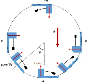
BITalino is equipped standardly with a micromechanical (MEMS) 3-axis accelerometer with measurement range of −3g/+3g [13, 14]. As often with this type of sensor, the accelerometer consists in a deformable beam (Fig. 1) with a small mass at one of its ends: measuring the beam deflection gives access to the force applied to the mass [13, 14]. This technique implies that the signal measured (beam deflection) has in fact two components. One is a “static” deflection due to gravity (Fig. 1) and is independent of the sensor acceleration. This component, equal to 𝑔𝑔 cos(𝜃𝜃), varies between −𝑔𝑔 and +𝑔𝑔, and this variation can be used for a simple sensor calibration [15]. The second component is a “dynamic” deflection due to the “real” acceleration (change of velocity) of the sensor in the axis direction. As explained below, this static component can be used to determine the oscillation amplitude.
Figure 1: Scheme of the static deflection of the cantilever beam due to gravity versus its orientation. The value read by BITalino (after calibration) is g cosθ.
The Python program used for this didactical work has the following functionalities, some common for this type of acquisition cards and others more specific to the pendulum experiment:
a) Graphical interface: a graphical user interface (GUI) displays a graph with the data measured by the BITalino for the acceleration in the three axes as a function of time. It also displays various (adjustable) parameters such as the sampling frequency and the minimum and maximum for each axis of the graph. This GUI is fundamental for testing the correct operation of the BITalino and of the mechanical setup as well as for some training and technical adjustments before starting data acquisition of the pendulum oscillations.
b) Calibration of the sensor: to obtain the sensitivity of the sensor ― expressed in (m/s2)/bit ― in
each direction (x, y, z), the BITalino must be slowly rotated to find the maximum and the minimum of the (static) accelerations. Once this is achieved, pressing an “OK” button assigns these extrema to the +𝑔𝑔 and −𝑔𝑔 values and determine the two constants necessary to transform the readings from the digital codes of the analog-to-digital (ADC) converter into the SI unit for acceleration (m/s2) [15].
c) “Save” button: this button stops the acquisition and save three files F1, F2 and F3 (standard ASCII text file). One, F1, ― with four columns ― corresponds to the raw data (as expressed in digital codes produced by the analog-to-digital converter) of the three-accelerometer axis as a function of time (BITalino internal clock). A second file, F2, is almost identical, except that the data recorded are directly expressed in m2/s using the last calibration performed. Depending of the student level and of the time allocated for the
work, the student can start the data analysis using one or the other file. The third file, F3, is very specific for the pendulum experiment. It provides five columns:
Column 1 and 2: The time corresponding to every other relative maxima of z-axis acceleration and the corresponding value in m2/s. As a matter of fact, it will be shown in section III that the period of
centripetal acceleration is half that of the oscillatory motion, that is why we choose to record the time and the amplitude of every other maxima in this auxiliary file;
Column 3 and 4: The time corresponding to every other relative minima of z-axis acceleration and the corresponding value in m2/s;
Column 5: The period of the oscillatory motion, calculated as the time difference between every other maxima. This period is calculated for each every other maxima recorded in the file.
Let us mention that the extrema of the acceleration are determined with a classical smoothing subroutine applied on the acquired data to facilitate their identification by minimizing the effects of noise and fluctuations (see next section). As a matter of fact, a reliable determination of extrema using basing functions available in common spreadsheet software being far to be obvious, we found necessary to provide these data to the student to avoid time consuming auxiliary operations.
2.2 Mechanical set-up
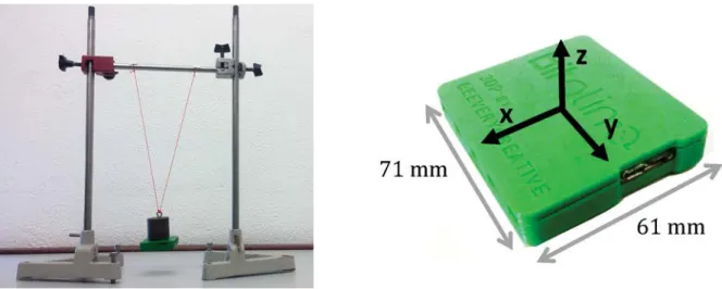
Figure 2 shows the experimental setup. The oscillating mass consists of a brass cylinder (m= 200 g to 600 g in our experiments) suspended on a metallic rod. The distance between the center of mass and the suspension point, L, was varied from 18 cm to 31 cm. The BITalino case was attached to the lower base of
the mass using double-sided adhesive tape allowing an easy (dis-)assembly, with its z-axis parallel to gravity when the mass is at rest. To minimize oscillations out of the plane perpendicular to the metallic rod, the mass was supported by two nylon wires as shown in Figure 2 and care was taken to maintain the BITalino z-axis in this plane when the mass was dropped from the maximum amplitude (initial angle, θ0, as
large as 60°, see below). Doing so, the oscillation take place in a unique plane, perpendicular to the rod, and its centripetal acceleration is measured by the accelerometer z-axis, az. Due to the relatively heavy masses
used and the large initial angles, it is difficult to avoid totally some oscillations and deformations of all this structure: to minimize such issues, the use of heavy rods and supports are recommended.
Figure 2. Left: global experimental set-up with the BITalino attached to the oscillating mass. Right: BITalino in its plastic case with its three axes, BITalino has a thickness of about 15 mm. The z-axis is perpendicular to the 61 mm × 71 mm face.
2.3 Typical results
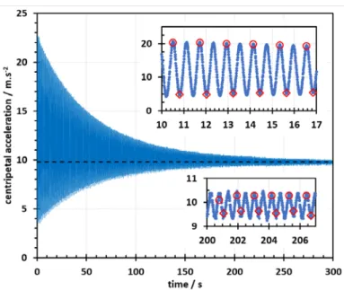
Figure 3 shows a typical result for centripetal acceleration using the system described in Figure 2 with a mass of 600 g and a distance L ≈ 31 cm. To obtain data on a large amplitude range, the motion was recorded during 5 min. To determine the period of the signal and the maxima and minima of acceleration with good accuracy, the data were acquired using a 100 Hz sampling rate. These two constraints lead to quite large files (about 30 000 lines) but still perfectly manageable by the current computers. The equilibrium value (dashed horizontal line) for az agrees with the expected value, 9.81 m/s2, for the static acceleration (Fig.
1). The main uncertainty comes from the calibration due to the 10-bit ADC: for a −3g/3g accelerometer, one bit corresponds to ≈ 0.06 m/s2. Before going further in the analysis, the following experimental
observations must be noticed:
i. the data are not symmetric with respect to the equilibrium value. Whereas the initial amplitude of the maximum acceleration is about 13 m/s2, the initial of the minimum
amplitude is about 6 m/s2;
ii. the period manually measured (“old fashion”, measuring visually the time over 10 periods, for instance) gives T≈ 1.1 s, close to the expected one, (2π�𝐿𝐿/𝑔𝑔 ≈ 1.12 s);
iii. the period of the BITalino signal (≈ 0.6 s) is approximately half of the visually measured.
Figure 3: Acceleration measured by BITalino vs time on a large (main plot) and short (insets) time scales. These measurements were performed using a 600 g mass for a distance L = 31.1 cm (Figure 2). The dashed horizontal line corresponds to az= 9.81 m/s2. This figure corresponds to the direct plot of the
data stored in files F2 (az(t), small symbols) and F3 (every other extrema de
az(t), open symbols).
This frequency doubling is easy to understand physically: for example, during one period of the motion, the centripetal acceleration reaches twice its maximum (upward direction) in θ = 0 (maximum linear velocity) and twice its minimum in 𝜃𝜃 = ±𝜃𝜃0 (null velocity). This frequency doubling will be derived
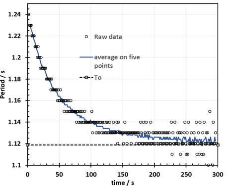
rigorously in section III. More information can be obtained in the auxiliary file F3 that gives the time at which occurs the every other maxima and minima of the acceleration as well as their respective value (open symbols in insets to Figure 3): the time determination is relatively trustworthy whereas the determination of the amplitude becomes not so accurate for small amplitudes. The period of the oscillatory motion is available in the same file and is plotted in Figure 4 (open symbols). The time measured by the BITalino being a multiple of the sampling period, its resolution is limited to 0.01 s, leading to a discretization, clearly visible in Figure 4. To mitigate this effect, a more continuous behavior for the period was obtained by calculating a moving average on five consecutive determinations (continuous line). This graph shows that twice the az period, as calculated in F3, is quite close to the calculated 2π�𝐿𝐿/𝑔𝑔 period or to the visually
determined one. This Figure 4 also shows that the period decreases with time: it will be analyzed in section 4 as a consequence of the amplitude decrease, the quantification of this effect being one of the objectives of this work.
These observations and experimental data can now be compared with the theory summarized in the following section.
Figure 4: The open circles represent the period of the oscillation ― twice the period of the acceleration (Cf. Figure 3) versus time, calculated by the Python program and stored in the F3 file. The continuous line is the moving average of the period calculated with five consecutive measurements. The dashed horizontal line shows the expected period (2π�𝐿𝐿/𝑔𝑔) for L = 31.1 cm and
g = 9.81 m/s2.
3 Centripetal acceleration for the simple pendulum
3.1 Period of a simple pendulum
Let us recall some characteristics of the canonical simple pendulum motion. A full and more detailed description of this system as well as its mathematic treatment can be found in many classical textbooks. The simple pendulum consists in a mass m suspended on a wire of length L ; if no other force than gravity 𝑚𝑚𝑔𝑔⃗ is applied, it obeys the differential equation
𝜃𝜃̈ + 𝜔𝜔02sin(𝜃𝜃) = 0 , Eq. 1
where θ = θ(t) represents the angle measured in respect to the vertical, and 𝜔𝜔0= �𝑔𝑔/𝐿𝐿 is the natural
frequency. In the small angle approximation, 𝜃𝜃 ≪ 1 (i.e., 𝜃𝜃 ≪ 60°), sin(𝜃𝜃) ≈ 𝜃𝜃 and Eq. 1 is easily solved: if the mass is deviated by 𝜃𝜃0 from its equilibrium position and released at t = 0 without initial velocity the
solution of Eq. 1 is
corresponding to an harmonic motion of period 𝑇𝑇0= 2𝜋𝜋�𝐿𝐿/𝑔𝑔. If the condition 𝜃𝜃 ≪ 1 is not fulfilled, it can
be shown that the period of the oscillations T becomes slightly amplitude dependent. One usual approximation for this dependence is given by [3, 4]:
𝑇𝑇−𝑇𝑇0 𝑇𝑇0 ≈ 1 16𝜃𝜃02+ 11 3072𝜃𝜃04 . Eq. 3
This equation indicates that the period decreases when the amplitude decreases, behavior in qualitative agreement with the results displayed in Figure 4, in which the initial period decreases by ≈ 10 % between the beginning and the end of the experiment. To verify quantitatively this Eq. 3, it is necessary to obtain the angular amplitude from the acceleration data displayed in Figure 3.
3.2 The centripetal acceleration of the pendulum
The centripetal acceleration 𝑎𝑎⃗centrip(𝑡𝑡), perpendicular to the tangential velocity 𝑣𝑣⃗ of the mass, will be
measured by the 𝑎𝑎𝑧𝑧 accelerometer. The mass describing a circular trajectory, it is given by:
𝑎𝑎centrip=𝑣𝑣 2
𝐿𝐿 . Eq. 4
Using 𝑣𝑣 = 𝐿𝐿𝜃𝜃̇ and calculating 𝜃𝜃̇ by Eq. 2a, the tangential velocity can be written as:
𝑣𝑣(𝑡𝑡) ≈ −𝐿𝐿𝜔𝜔0 𝜃𝜃0sin(𝜔𝜔𝑜𝑜𝑡𝑡) . Eq. 5a
Using this expression and 𝜔𝜔0= �𝑔𝑔/𝐿𝐿,
𝑎𝑎centrip(𝑡𝑡) =𝑣𝑣 2 𝐿𝐿 = 𝑔𝑔𝜃𝜃02sin2(𝜔𝜔0𝑡𝑡) = 𝑔𝑔𝜃𝜃02� 1 2− cos (2𝜔𝜔0𝑡𝑡) 2 � . Eq. 6a
Before going further, let us note that this last equation confirms that the centripetal acceleration oscillates at a frequency twice higher than that of the motion 𝜔𝜔0: mathematically, the reason is that 𝑎𝑎centrip
depends quadratically upon the tangential velocity, this one oscillating at 𝜔𝜔0. This is a special case of a very
general rule in physics: non-linear effects lead to the appearance of new frequencies.
3.3 The centripetal acceleration of the damped pendulum
To describe the motion damping, a viscous force 𝐹𝐹⃗ = −𝑏𝑏𝑣𝑣⃗ is usually introduced and a term (1 𝜏𝜏)⁄ 𝜃𝜃̇, in which τ = b/m is the damping time, appears in the left-hand side of Eq. 1. In the case of weak damping (i.e. 𝜔𝜔0𝜏𝜏 > 1) the solution of the modified Eq. 1 becomes (same initial conditions, 𝜃𝜃(0) = 𝜃𝜃0, 𝑣𝑣(0) = 0)
𝜃𝜃(𝑡𝑡) = 𝜃𝜃0𝑒𝑒−𝑡𝑡/𝜏𝜏cos(𝜔𝜔𝑡𝑡) = 𝜃𝜃max(𝑡𝑡) cos(𝜔𝜔𝑡𝑡) , Eq. 2b
in which 𝜔𝜔2= 𝜔𝜔 0
2(1 − 1
(𝜔𝜔0𝜏𝜏)2). In Eq. 2b, 𝜃𝜃max(𝑡𝑡) represents the amplitude of the oscillation that decreases
exponentially with time due to the viscous force. The tangential velocity can be calculated as
𝑣𝑣(𝑡𝑡) = −𝐿𝐿𝜏𝜏𝜃𝜃0𝑒𝑒−𝑡𝑡/𝜏𝜏�1 + (𝜔𝜔𝜏𝜏)2sin (𝜔𝜔𝑡𝑡 + 𝛽𝛽) Eq. 5b
with 𝑡𝑡𝑎𝑎𝑡𝑡 𝛽𝛽 = 1/𝜔𝜔𝜏𝜏.
In the case of very weak damping, 𝜔𝜔𝑜𝑜𝜏𝜏 ≫ 1 (it will be verified latter that this condition is fulfilled
in our experimental setup), the terms of higher order than 1/(𝜔𝜔𝜏𝜏) can be dropped and the centripetal acceleration is given by:
𝑎𝑎centrip(𝑡𝑡) =𝑣𝑣 2 𝐿𝐿 ≈ 𝑔𝑔𝜃𝜃𝑜𝑜2 𝑒𝑒 −𝜏𝜏/2𝑡𝑡 sin2(𝜔𝜔 𝑜𝑜𝑡𝑡) = 𝑔𝑔𝜃𝜃𝑜𝑜2𝑒𝑒− 𝑡𝑡 𝜏𝜏/2�1 2− cos (2𝜔𝜔𝑜𝑜𝑡𝑡) 2 � Eq. 6b
Within this very weak damping approximation, the main difference in respect to Eq. 6a (no friction) is the attenuation factor, 𝑒𝑒−𝜏𝜏/2𝑡𝑡 , coming from viscous force.
3.4 Extrema of the measured acceleration
As explained in section 2-1, the acceleration given by Eq. 6b corresponds to the “real” acceleration (change of velocity) of BITalino and the signal measured by the BITalino, 𝑎𝑎𝑧𝑧(𝑡𝑡), is actually the sum of this real
acceleration and of the component corresponding to the “static” deflection 𝑔𝑔cos(𝜃𝜃(𝑡𝑡)): 𝑎𝑎𝑧𝑧(𝑡𝑡) = 𝑔𝑔𝜃𝜃02𝑒𝑒−
𝑡𝑡
𝜏𝜏/2 sin2(𝜔𝜔0𝑡𝑡) + 𝑔𝑔 cos(𝜃𝜃0𝑒𝑒−𝑡𝑡𝜏𝜏cos(𝜔𝜔0𝑡𝑡)) . Eq. 7
Instead of trying to fit the experimental data to this analytical expression1, let us focus on the extrema of
𝑎𝑎𝑧𝑧(𝑡𝑡).
Maxima of acceleration: They occur when the mass passes through its rest position with its maximum velocity and then maximum centripetal acceleration. They corresponds to 𝜃𝜃(𝑡𝑡) = 0, i. e. 𝜔𝜔0𝑡𝑡 =
π 2⁄ + 𝑡𝑡π (Eq. 2b). From Eq. 7:
𝑎𝑎𝑧𝑧,max(𝜃𝜃 = 0) = 𝑔𝑔𝜃𝜃02𝑒𝑒− 𝑡𝑡
𝜏𝜏/2+ 𝑔𝑔 . Eq. 8
The amplitude of these maxima decreases exponentially with a relaxation time equal to τ/2. Fitting this
relaxation time gives access to τ and to 𝑔𝑔𝜃𝜃02: 𝜃𝜃
0 can be obtained as well as the angular amplitude versus
time, 𝜃𝜃0𝑒𝑒−𝑡𝑡/𝜏𝜏.
Minima of acceleration. These minima occur when the mass velocity is null, i.e., when the mass reaches its maximum of amplitude 𝜃𝜃max corresponding to 𝜔𝜔0𝑡𝑡 = 𝑡𝑡π (Eq. 2b). In these cases, 𝑎𝑎𝑧𝑧 measures
only the “static” contribution and the envelope of these minima is given by 𝑎𝑎𝑧𝑧,min (𝜃𝜃 = 𝜃𝜃max) = 𝑔𝑔 cos �𝜃𝜃0𝑒𝑒−
𝑡𝑡
𝜏𝜏� . Eq. 9
Note that the asymmetry of the data in respect to the equilibrium value highlighted in section 2.3 are explained by the equations 8 and 9: the positive and negative extrema of 𝑎𝑎𝑧𝑧(𝑡𝑡), as well as their damping
times, are different.
1 Let us note that, because actually the period decreases with amplitude, this fit would not be so trivial.
Figure 5: Theoretical (Eq. 8 and 9) and experimental (Python determination) values of the extrema of 𝑎𝑎𝑧𝑧. The adjustment of the theoretical determination to
the experimental data of the maxima led to 𝜃𝜃0= 65° and τ= 115 s. These same
values are used to calculate the theoretical minima.
4 Analysis of the experimental results
4.1 Damping time determination
In Figure 5, the experimental data for the extrema of az(t) saved in the auxiliary file F3 are compared with
the analytical expression given by the equations 8 and 9 with 𝜃𝜃0 and τ as adjustable parameters. In the
upper part of this figure, are plotted these experimental data for the maxima (decreasing red thick line), as well as the equation 8 (decreasing black thin line). By a try-and-error process, a very good agreement between these two types of data is found, leaving, in the case of this experiment, to 𝜃𝜃0= 65° and τ= 115 s.
In the lower part of the same graph are plotted the experimental values for the minima (increasing green thick line) as well as the equation 9 (thin black line) with the same values for (𝜃𝜃0,τ ): a very good agreement
is also obtained. Let us remind that these two sets of measurements (maxima and minima of 𝑎𝑎𝑧𝑧) are indeed
independent, each one measuring a different effect (one measures the centripetal acceleration at θ = 0, the
other one measures the maximum inclination of the pendulum), the agreement between the two calculated curves and the corresponding experimental data must be taken as a proof of the quality of the recorded data. Let us however mention that a value τ= 110 s could describe slightly better (visual evaluation) the
evolution of the minima value versus time.
Using this quite good experimental determination of τ, this damping time was measured for various
systems using different wire length and mass. The results for 𝜔𝜔0 and τ are indicated in Table 1. First, let us
note that the condition 𝜔𝜔0𝜏𝜏 ≫ 1 is always satisfied (last column of Table 1): our system is very lightly
3.3 are fully justified. Frequently, in practical classes, the pendulum period is measured for various length
L and these data are used to verify the T vs𝐿𝐿1/2 law and to deduce the gravity acceleration. Using the data
of table 1, the T vs.𝐿𝐿1/2 slope gives ≈ 2.017 s kg−1/2, leading to g ≈9.71 m/s22. This ≈ 1 % discrepancy could
come from the imprecision on the L measurement, or by the fact that, in our case, the oscillating mass is not so small compared to 𝐿𝐿 and the 𝑇𝑇 = 2π�𝐿𝐿/𝑔𝑔 law have to be refined taking into account its real moment of inertia, such an analysis is out of the scope of this article but could also be included in a more complete work. Whereas a viscous force implies τ ∝ 𝑚𝑚, our data shows that τ decreases with m indicating that, in
our system, the damping is caused by other effects: for example, the friction of the wire on the metallic rod as well as the energy lost by deflecting the relative light supporting rods during the motion could be the main source of energy dissipation but, once again, further analysis is beyond the scope of this paper.
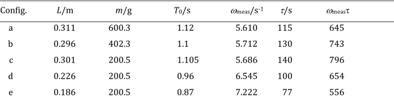
Table 1: Experimental results for angular frequency measured (ωmeas) from period at small
amplitude (T0) and damping time for different configurations (wire length and oscillating mass).
Config. L/m m/g T0/s ωmeas/s-1 τ/s ωmeasτ
a 0.311 600.3 1.12 5.610 115 645
b 0.296 402.3 1.1 5.712 130 743
c 0.301 200.5 1.105 5.686 140 796
d 0.226 200.5 0.96 6.545 100 654
e 0.186 200.5 0.87 7.222 77 556
4.2 Period versus amplitude
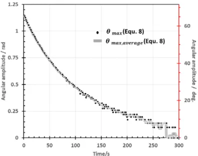
The Equations 8 and 9 allow to extract the angular amplitude, 𝜃𝜃max(𝑡𝑡) = 𝜃𝜃0𝑒𝑒−𝑡𝑡/𝜏𝜏, at each extremum
from the acceleration data. For instance, 𝜃𝜃max(𝑡𝑡) obtained from the experimental acceleration maxima
𝑎𝑎𝑧𝑧,max displayed in Fig. 5 and using Eq. 8 are plotted on Figure 6. 𝜃𝜃max(𝑡𝑡) calculated by the minima of the
acceleration (Eq. 9) was also computed and lead to very similar results [9], they are not displayed in this figure for sake of clarity. To obtain a less noisy data set, especially for low amplitude, this amplitude was averaged on 5 periods (θmax, average- thick grey line) exactly as done for the period smoothing process.
Moreover, doing so, each period averaged (data of Fig. 4) can be associated with the corresponding averaged amplitude (data of Fig. 6) then the dependence of the period 𝑇𝑇 upon θmax can be obtained as
displayed on figure 7a.
2 Along this article, no error handling is presented: it would turn it heavier and without real benefits
in respect to the main goal of this article that is to show that this setup is a good tool for studying pendulum physics. Error handling can be included in the full work to be performed by the students
Figure 6. The symbols indicate the angular amplitude, 𝜃𝜃max(𝑡𝑡), versus time
obtained from Eq. 8. The thick grey solid line corresponds to 𝜃𝜃max,average,
moving average calculated by Eq. 8 on 5 consecutive periods.
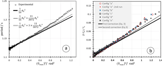
Considering Eq. 3, in Figure 7a, the average period was plotted as a function of 𝜃𝜃ma𝑥𝑥,average2 . In first
approximation, a quadratic dependence of the period in 𝜃𝜃max described quite well the experimental data.
In this figure, the thick black line represents the first correction predicted by Eq. 3 and its value is in quite good agreement with the measurements, especially at low amplitude. However, for higher amplitude, the departure from this quadratic dependence is larger than the quartic correction proposed by Eq. 3 (thin black line): a quartic correction three times larger than proposed by Eq. 3 described very well these data (thick grey line). As already mentioned, the fact that the oscillating mass cannot be considered as point-like should be considered for a finer description of this 𝑇𝑇(𝜃𝜃max) behavior. The 𝑇𝑇(𝜃𝜃max) dependences were
measured for the various configurations (L, m) listed in Table 1. They are displayed in Figure 7b and show that, within the uncertainties of our measurement, the quadratic and quartic corrections seem at first sight independent of mass and length as predicted by Eq. 3. A more complete analysis is beyond the scope of this work but seems to be possible using this experimental setup.
Figure 7: Period of oscillation versus the square of the angular amplitude 𝜃𝜃max2 .
Figure 7a: for the L = 31,1 cm and m = 600 g configuration. Note the very good agreement with the first correction of Eq. 3 (thick black line) for small angle. For angle higher than ≈ 0.7 rad (≈ 40°), the experimental results follow (thick gray line) a dependence three times larger than predicted (thin black line). Figure 7b: Relative change of period for the various configuration listed in table 1.
5 The pendulum and the BITalino in the framework of the classroom
The work described in the previous sections can be easily adapted to various educational levels (from high school to 1st cycle of university) or to the time allocated for practical session. The analytical expressions of
section 3 can be either obtained by the students or given by the teacher and discussed with the students using elementary knowledge about the damped pendulum. It is important to highlight that measuring the centripetal acceleration and using a cantilever induces some “unintuitive results”. For instance, depending on the teaching strategies, the frequency doubling of the measured signal can be deduced by the students before experiments or, on the contrary, can be discovered and explained by the students during the experimental work. Total duration of 4-6 hours seems to us reasonable to perform all the work. This duration includes the software installation, the calibration of the sensors, some training and tests and the data acquisition with different masses and lengths. If necessary, these 4-6 hours can be divided in two different sessions, the first one dedicated to the installation and training, the second to data acquisition and basic analysis. Student skills in data analysis using spreadsheets are frequently not as developed as expected: this work is a good opportunity to use spreadsheets to make mathematical data processing as well as to compare theory with experimental results. In the version we described in this article, we chose to provide to the student the software that calculates the period of the signal as well as the time stamps of the extrema turning usual spreadsheets adequate for data analysis. However, for students with some knowledge of computer programming, this program can be part of the work or a complementary work done in collaboration with informatics class: data smoothing and extrema detection is a useful and enriching exercise.
From the point of view of the teacher, the experimental setup is very simple and inexpensive to install (Figure 2). The wireless capability leads to a very clean experimental site without irritating problems due
to faulty wires, cables or contacts. In this experimental set-up, no complicate mechanism is needed for the angle measurement, its value being determined by the accelerometer. Moreover, the same acquisition board can be used for many other applications within the practical class and is then very easily finantially amortized. For instance, in the framework of a didactical experiment dedicated to magnetic induction phenomenon [9], this same board, coupled to a simple homemade amplifier, was used as a microvoltmeter to measure low voltage (10-300 µV range) versus time. Other properties or signals can be measured by built-in sensors or using the analogical inputs existing in general in such type of devices. For us, beyond their relatively reduced price, one of the main advantages of using such boards is really their versatility: it avoids problems frequently encountered in our physics lab such as compatibility between apparatuses of different brands, limitation due to “closed” software and so on. The students and/or the teacher can really build their own experiment, with their own material and with their own ideas.
6 Conclusion
Modelling is in the essence of physical sciences [16]. Most physical models are expressed as equations and becoming familiar with the process of creating these equations is an essential task in learning science and engineering. The pendulum study is a good way to train this creating process. We showed in this paper that the experimental results obtained with a low-cost data acquisition card, incorporating wireless communication and accelerometer sensors as it is quite common nowadays, are accurate and useful to go beyond the basic theory of the simple pendulum: by measuring the acceleration, the damping time, as well as the dependence of the period with amplitude, are obtained with good precision. To allow comparison with the usual theoretical predictions, the data has to be analyzed using a spreadsheet and various calculation steps, contributing to improve student skills with this type of general computational tools. Beyond this mathematical analysis, some of these results, namely the non-symmetrical az(t) behavior as
well as the frequency doubling, can be understood after some reflection needed by the fact that the centripetal acceleration is not related to the oscillation angle by an obvious way. We take this reflection (accompanied or not by the mathematical demonstration) as an added value to the usual pendulum lab assignments.
Sometimes, to generate an extra motivation and some enthusiasm, it is necessary to introduce or explain to the students the practical work using some exciting ideas. With the work presented here, the very classical simple pendulum experiment became, in our opinion, more attractive and challenging than some typical didactical pendulum works. More attractive because the measurements are performed using a microelectromechanical device currently used in many domains other than physics laboratories (including their very beloved cell cell-phones!). It is important that the student becomes familiar with hardware used outside schools. Attractive also because the acquisition board used in this experiment is wireless, very versatile and can be used for many other types of measurements. Unfortunately, in teaching laboratories, many experimental apparatuses are exclusive of these labs. Using devices that can be used for other purposes helps to build the idea that physics labs are useful not only to test or “discover” physical laws but also as an introduction to other type of measurements in “real life”. More attractive also because this work avoids studying one of the more fascinating and fundamental physics problems by the angle
measurement that seems the most obvious way… so obvious that it could seem, a priori, tedious3. Studying
this motion by measuring the centripetal acceleration offers an alternative to this “obvious” solution. However, as mentioned in the introduction, acceleration is not as intuitive as linear or angular position. For instance, it is very probable that a student will take as evident that the periodicity seen on Figure 3 is the periodicity of the motion. A rapid measurement will show that this spontaneous guess is wrong, as the asymmetric results displayed on Figure 3 were also, at first sight, not expected. A full explanation of these “not obvious results”, without any calculations, would be a challenge for the sagacity of the students.
Because neither expensive apparatus nor special materials are needed except the acquisition board, the experimental setup can be installed on any site other than the classroom. An alternative way to the classical work performed in a classical physics laboratory could be to say to the students: “Here is an acquisition card with an integrated accelerometer, build something to put some mass to oscillate, fix the acquisition board to it and come back with the parameters of your own damped oscillator!”.
7 References
1) Matthews M.R. (2014) Pendulum Motion: A Case Study in How History and Philosophy Can Contribute to Science Education. In: Matthews M. (eds) International Handbook of Research in History, Philosophy and Science Teaching. Springer, Dordrecht; DOI 10.1007/978-94-007-7654-8_2,
2) See for instance: Halliday, Resnick, Walker (2013) Fundamentals of Physics (10th edition),. Wiley Editorial,
Chapter 15
3) A. Beléndez, T. Hernández, A. Beléndez, and C. Neipp, “Analytical approximations for the period of a nonlinear pendulum,” Eur. J. Phys. 27, 539–551, 2006.
4) For rapid calculation of 𝑇𝑇(𝜃𝜃0) given by [3]: http://hyperphysics.phy-astr.gsu.edu/hbase/pendl.html 5) See for instance: https://www.ld-didactic.de/en/catalogues/physics/physics-experiments.html
6) A. Godfrey, T. Hourigan, G. M. ÓLaighin 2007 Pendulum analysis of an integrated accelerometer to assess its suitability to measure dynamic acceleration for Gait applications 29th Annual Int. Conf. of the IEEE EMBS, Cité Internationale (Lyon, France, 23–26 August), (https://doi.org/10.1109/IEMBS.2007.4353436)
7) J. Briggle 2013 Analysis of pendulum period with an iPod touch/iPhone, Phys. Educ. 48 285
8) A. M. Pendrill and J. Rohlén 2011 Acceleration and rotation in a pendulum ride, measured using an iPhone 4, Phys. Educ. 46 676
9) J. Alho, Development of didactic physics experiments using a miniaturized wireless acquisition board, Physical engineering master thesis, Universidade Nova de Lisboa 2017. http://hdl.handle.net/10362/28551 10) João C Fernandes et al 2017 Study of large-angle anharmonic oscillations of a physical pendulum using an acceleration sensor, Eur. J. Phys. 38 045004
11) H. Plácido da Silva, A. Fred and R. Martins 2014, Biosignals for Everyone. IEEE Pervasive Computing, 13(4):64-71, 2014
12) Nogueira P., Urbano J., Reis L.P., Cardoso H.L., Silva D., Rocha A.P. (2017) A Review Between Consumer and Medical-Grade Biofeedback Devices for Quality of Life Studies. In: Rocha Á., Correia A., Adeli H., Reis L., Costanzo S. (eds) Recent Advances in Information Systems and Technologies. WorldCIST 2017. Advances in Intelligent Systems and Computing, vol 570. Springer, Cham
13) Albarbar A., Teay S.H. (2017) MEMS Accelerometers: Testing and Practical Approach for Smart Sensing and Machinery Diagnostics. In: Zhang D., Wei B. (eds) Advanced Mechatronics and MEMS Devices II. Microsystems and Nanosystems. Springer, Cham. doi.org/10.1007/978-3-319-32180-6_2
14) http://www.analog.com/media/en/technical-documentation/data-sheets/ADXL335.pdf 15) http://bitalino.com/datasheets/REVOLUTION_ACC_Sensor_Datasheet.pdf
16) Ronald N. Giere 1988 Explaining Science: A Cognitive Approach. Chicago, Science and Its Conceptual Foundations series, The University of Chicago Press.
3 The pendulum is sometimes used to fall people asleep!