(1) Received for publication in September 9, 2010 and approved August 31, 2011.
(2) D. Eng. in Agricultural Engineering at the State University of West Paraná, Universidade Estadual do Oeste do Paraná – UNIOESTE, Paraná, Brazil. E-mail: [email protected]
(3) Associate Professor of the Graduate Program in Agricultural Engineering at the State University of West Paraná, UNIOESTE. E-mail: [email protected]
(4) D.S Professor at the Dept. of Mathematics, Catholic University (Universidad Católica) Santiago - Chile. E-mail: [email protected]
LOCAL INFLUENCE FOR SPATIAL ANALYSIS OF SOIL
PHYSICAL PROPERTIES AND SOYBEAN YIELD USING
STUDENT’S
t-DISTRIBUTION
(1)Rosangela Aparecida Botinha Assumpção(2), Miguel Angel Uribe Opazo(3) & Manuel Galea(4)
SUMMARY
The modeling and estimation of the parameters that define the spatial dependence structure of a regionalized variable by geostatistical methods are fundamental, since these parameters, underlying the kriging of unsampled points, allow the construction of thematic maps. One or more atypical observations in the sample data can affect the estimation of these parameters. Thus, the assessment of the combined influence of these observations by the analysis of Local Influence is essential. The purpose of this paper was to propose local influence analysis methods for the regionalized variable, given that it has n-variate Student’s t-distribution, and compare it with the analysis of local influence when the same regionalized variable has n-variate normal distribution. These local influence analysis methods were applied to soil physical properties and soybean yield data of an experiment carried out in a 56.68 ha commercial field in western Paraná, Brazil. Results showed that influential values are efficiently determined with n-variate Student’s t-distribution.
RESUMO: INFLUÊNCIA LOCAL PARA ANÁLISE ESPACIAL DOS ATRIBUTOS FÍSICOS DO SOLO E DA PRODUTIVIDADE DA SOJA UTILIZANDO A DISTRIBUIÇÃO t-STUDENT
A modelagem e estimação dos parâmetros que definem a estrutura de dependência espacial de uma variável regionalizada, utilizando métodos geoestatísticos, é de fundamental importância, pois a partir desses parâmetros é realizada a krigagem dos pontos não amostrados para a construção dos mapas temáticos. A presença de uma ou mais observações atípicas nos dados amostrais podem influenciar a estimação desses parâmetros. Assim, torna-se importante a avaliação da influência conjunta destas observações pela análise de Influência Local. Este trabalho tem por objetivo apresentar métodos de análise de influência local para variável regionalizada considerando que ela tenha distribuição t-Student n-variada e comparar com a análise de influência local considerando que esta mesma variável regionalizada tenha distribuição normal n-variada. Esses métodos de análise de influência local foram aplicados a atributos físicos do solo e produtividade da soja obtidos a partir de um experimento realizado em uma área comercial de 56,68 ha da região Oeste do Paraná, Brasil. O estudo mostrou que os valores influentes são identificados eficientemente com a distribuição t-Student n-variada. Termos de indexação: geoestatística, algoritmo EM, variabilidade espacial.
INTRODUCTION
Geostatistics is an important tool to analyze spatial variability of soil properties and crop yield. Thematic maps based on geostatistics are excellent resources for the analysis of agricultural performance, and are considered the most complete option for the zoning of crop spatial variability (Molin, 2002). However, when the data set contains influential values, the maps diverge from reality and can therefore cause misinterpretation.
The identification of influential observations in the data set is known as diagnostic analysis (Paula, 2004) and was presented by Cook (1986) as a new method called “Local Influence” for diagnostic analysis of the Gaussian process. This analysis was based on the assumption that the model is reliable, and analyzed the power of conclusions for data or model disturbances.
Several studies of spatial analysis have been developed using diagnostic techniques to find observations that influence model sets. Christensen et al. (1992, 1993) worked on studies that analyzed the prediction of parameters in linear spatial models by applying diagnostic techniques to find observations that can influence the estimation of the covariance matrix, used in universal kriging. Militino et al. (2006) tried to identify outliersin multivariate linear spatial models. Borssoi et al. (2009, 2011) conducted diagnostic studies of linear Gaussian spatial models, and developed several measures of local influence.
The purpose of this paper was to propose a method that uses n-variate Student’s t-distribution with a fixed degree of freedom and also uses the maximum likelihood function as method of estimating spatial
variability parameters of soybean yield. From the estimation of these parameters, a study of local influence is developed, which analyzes the existence of influential observations in the spatial dependence structure (graph Ci) and in the linear predictor (graph lp), considering the yield itself as explicative variable and soil penetration resistance (SPR) and soil density (Des) as covariates. Finally, these results were compared with those obtained by using the n-variate normal distribution.
THEORY Student’s t linear spatial models
Let {Y(s), s∈S} be a stationary stochastic process, where S ⊂ℜd and ℜd is a d-dimensional (d≥ 1)
Eucledian space. The Y = (Y(s1),…, Y(sn))T process
has n-variate t-distribution with
v
degrees of freedom (v ≥ 1 fixed), where µ is the vector of location parameters and ∑ the scaling matrix, ie Y ~ tn(µ,∑,v).Consider that Y = (Y(s1),…, Y(sn)T are registered at
known locations in space known in si and sj for i≠j =
1,…,n. Each Y(si) can be written as:
Y(si) = µ(si) + ε(si), i = 1,…, n (1)
where µ(si) is a deterministic and ε(si) a stochastic term, both depending on the parameter space where
Y(si) operates. It is assumed that the stochastic error
ε has zero mean, ie, (si) = E[ε(si)] = 0, i = 1,…, n and
that the variation of the points in space is determined by a covariance function C(.) of si and sj. This
covariance function is also specified by a parameter vector Φ = (ϕ1,ϕ2,ϕ3)T, which are the parameters that
For some known functions of S, such as
X1(s),…,Xp(s), we consider the linear spatial model in
the mean of the process µ(.), as: µ(si)= βjXj(si), i =
1,…, n, whereas X1 is a vector of um’s, X2,…,Xp are the covariables and β1,…,βp are unknown parameters.
Equation (1) can be written in matrix form,
Y = Xβ + ε (2)
where Y = (Y(s1),…,Y(sn))T and ε = (ε(s
n))T are vectors nx1, µ = Xβ is a vector nx1, X is a matrix n x p
composed by the vector of um’s and by (p–1) covariates and β = (β1,…,βp)T is the vector of unknown
parameters to be estimated.
Random error vector expectation ε, E(ε) = 0 is a zero vector, and its scaling matrix is Σ = [(σij)], where σij = C(si, sj).
Assuming Σ is not singular and that the matrix X
is full rank (rank (X) = p), the scaling matrix Σ can assume a spatial structure of:
Σ = [(σij)] = ϕ1ln + ϕ2R (3)
where ln is the identity matrix nxn, ϕ1 is the
parameter that determines the nugget effect, ϕ2 is
the parameter that defines the sill or contribution, R
= R(ϕ3) is a symmetric nxn matrix, and the reach a
is a function of ϕ3, ie α = g(ϕ3).
The elements i and j of the matrix Σ are C(si,sj) =
C(hij) = ϕ2rij, where hij = si –sj, whereas the elements rij are from the matrix R of the form for i ≠j and rij = 1, for i = j = 1,…, n.
The joint probability density function of Y is:
(4)
where Γ(.) is the gamma function. For v > 1, µ = Xβ
is the vector of means and for v > 2, is the covariance matrix.
Let θ = (βT ΦT)T be the vector of unknown
parameters and Y the vector of the observed data, where Y ~ tn(Xβ,Σ,v) with fixed v. The likelihood
function logarithm of the observed data Y in relation to θ is given by
Algorithm for parameter estimation (EM algorithm)
The parameter vector θ = (βTΦT)T is estimated by
the EM algorithm, based on the mixture of normal distribution that obtains Student’s t-distribution (Liu & Rubin, 1995).
We consider Yc = (Y,Ym) as the complete data set
with a parameterized density f(Yc |θ) by a vector of n -dimensional parameters, θ∈Θ⊂ℜs, with s=p+q (q=3),
where, Y and Ym are the observed and non-observed
data, respectively. The maximum likelihood estimate (ML) of θ can be obtained based on the complete data of the likelihood function log and the EM algorithm (Dempster et al., 1997). This algorithm consists of two steps: Expectation (Step E) and Maximization (Step M).
Step E: Q(θ|θ(r)) = E{L
c(θ|Yc)|Y,θ(r)} is defined; at this
step the expectation Q(θ|θ(r)) results from conditional
distribution f(Ym|Y,θ(r)) in the rth iteration.
Step M: θ(r+1) = Arg max
θQ(θ|θ(r)); at this step a
θ(r+1) is determined, which maximizes Q(θ|θ(r)). The
sequence derived from the EM algorithm iterations converges to the likelihood maximum estimate of .
Local influence
A perturbation vector ω = (ω1,…,ωn)T is considered,
varying in a region Ω⊂ℜd, used as additive
perturbation of Yω = Y + ω. Let the likelihood function be L(θ,ω|Y) in the observed data and Lc(θ,ω|Yc) in the
complete data for the perturbed model and assuming that there is ω0 so that L(θ,ω0|Y) = L(θ|Y) and
Lc(θ,ω0|Yc) = Lc(|Yc) for every θ, and also that (ω0) is
the ML estimator of θ for L(θ,ω|Y). Cook (1986) considers the displacement of the likelihood function log LD(ω) = 2[L( |Y) – L( (ω)|Y)] to assess the local influence of a small perturbation. Due to the difficulty of its application to complicated models, Zhu & Lee (2001) proposed an option with a shift function for
LD(ω), defined by fQ(ω) = 2[Q( | ) – Q( (ω)| )], where (ω) is the estimate of θ that maximizes Q( ,ω| ) =
E[Lc(θ,ω|Yc)Y, ]. The local influence graphic of fQ(ω) is defined as α(ω) = [ωT,f
g(ω)]T. In this case, the normal
curve Cfg,l of α(ω) in ω0 in the direction of some unit
vector l can be used to summarize the local behavior of fQ(ω). The normal curvature CfQ,l for α(ω) and ω0
is defined: CfQ,l = 2[lTΔTω0{– θ( )}-1Δω0l], where θ( )
= ∂2Q(θ,| )/∂θ∂θT
|θ= and Δω0 = ∂2Q(θ,ω0| )/∂θ∂ωT|θ= (ω).
Poon & Poon (1999) include the conformal normal curvature ΒfQ,l for ω0 in the direction of some unit
vector l, such as:
(5)
where ω0 = ∂2Q( (ω)| )/∂ω∂ ωT|ω=ω0, and BfQ,l is a
Given the matrix BfQ,l and considering
Ci = 2*|bii| (6)
where bii are the elements of the main diagonal of
matrix BfQ,l, we find graph Ci according to order i,to analyze the existence of influential observations in the spatial dependence structure. Zhu & Lee (2001) stated that for Ci, the ith point is influential in the
spatial dependence structure if:
, for i,j=1,…, n (7)
where bii is an element of matrix BfQ,l,
and .
In the study of spatial data, universal kriging has been used as a measure of prediction, to obtain values for the regionalized variable at non-sampled points. Let Y0 = Y(s0) be the universal kriging predictor of
location s0∈S. The mean of Y0 is given by , where = (x01,…,x0p) and x0j = xj(s0) for j = 1,…,p.
The predictor of the least mean square error is given by
thus , with hi0 = si – s0 for i =
1,…,n.
Thus, we have S(l) = lT (s
0,θ), where (s0,θ) is a
vector n x1 given by
(8)
In equation (8) we have
where and ,
thus and
for j = 1,2,3.
The direction of maximum local slope for the linear predictor is given by equation (9)
(9)
Graph is used to assess the influence on the linear predictor,
MATERIAL AND METHODS
The experimental data were collected in the 2004/ 2005 growing season, through a research that was conducted in a field of commercial grain production (56.68 ha) in Cascavel, in western Paraná (approx. 24.95º S, 53.57º W, 650 m asl). The soil was classified as a clayey Oxisol (specifically Latossolo Vermelho distroférrico), with a long-term crop succession of oat in the winter and soybean in the summer. The local climate is mild, mesothermal, and super humid, Cfa (Köppen classification), with moderate temperatures and well-distributed rainfall. The mean winter temperature is below 16 °C, with possible frost, and summers are hot, with temperatures above 30 ºC.
The soybean variety COODETEC 216 (CD216) was planted in no-tillage in the experimental area. For the study, 47 plots were marked, all of which were georeferenced using a Trimble GeoExplorer 3 GPS receiver (Global Positioning System) and the static method with post-processed differential correction, for the correct location in the spatial system of geographic coordinates Universal Transverse Mercatur (UTM), using metric coordinates.
From each of the 47 plots, the following data were collected: soybean yield (Prod) [t ha-1], soil density (Des)
[kg dm-3] in the layers 00–10, 10–20 and 20–30 cm
and soil penetration resistance (SPR) [MPa] in the same layers.
The Des was determined by the volumetric ring method (Kiehl, 1979), where one repetition was applied per depth per sampling. The SPR in the layers examined was measured with a penetrometer (SC-60, Soil Control; shaft 600 mm, diameter 9.53 mm), equipped with a cone at the tip (base area 129.3 mm², diameter 12.83 mm, corner angle 30°). A mean value of mechanical resistance to penetration was calculated based on four random replications per location and experimental plot.
Initially, descriptive statistics were obtained for the variables: soybean yield (Prod), and penetration resistance, and density in the soil layers 00–10, 10–20, and 20–30 cm deep (RSP0–10, RSP10–20, e RSP20–30;
Des0–10, Des10–20 e Des20–30, respectively) to assess their
behavior, identify the presence of discrepant points and possible causes.
and
where β1,…,β1 and ϕ1,ϕ2, ϕ3 are the unknown
parameters to be estimated.
The cross-validation criterion, Akaike information criterion (Faraco et al., 2008), and the maximum value of the log-likelihood function (LLF) were used for the choice of model space. Local influence analysis was performed to identify influential points. Universal kriging interpolation of the variable under study was the final step along with the creation of thematic maps. For data analysis software R (R Development Core Team, 2005) was used, and its modules geoR (Ribeiro JR & Diggle, 2001) and Splancs (Rowlingson & Diggle, 1993).
RESULTS AND DISCUSSION
The soybean yield mean was 3.23 t ha-1, standard
deviation SD = 0.38 t ha-1 and the coefficient of
variation CV = 11.79 %, identifying data homogeneity. With increasing depth, the covariate of soil penetration resistance (SPR) decreased the values of the mean, first quantile (Q1), median and trird qualite (Q3), and
increased akewness and kurtosis. It was observed that for SPR, in all layers, there are sample data above 2.60 MPa and that in RSP0–10, 50 % of the data were
over 2.64 MPa. According to Canarache (1990), SPR values in the range [1.1 to 2.59] MPa are not very restrictive for roots, but root-limiting in the range [2.6 to 5.0] MPa. It was also observed that the standard deviation of SPR does not vary much in the three layers, remaining within 0.49 and 0.56 MPa.
The three layers have homogeneity (coefficient of variation below 30 %). For soil density (Des), all statistical measures showed increases from layer 0– 10 cm to layer 10–20 cm, and reduction in statistical measures from layer 10–20 cm to layer 20–30 cm, which features a compacter layer below the soil surface, that prevents water infiltration. The mean, standard deviation, and density coefficient of variation do not change much in the three layers. As for SPR, homogeneity was observed for Des in the three layers (coefficient of variation below 30 %).
Coefficients of skewness and kurtosis were calculated. In covariates RSP20–30, Des10–20, and
Des20–30, the calculated coefficients do not belong to the 95 % skewness and kurtosis coefficient confidence intervals constructed by Jones (1969) that characterize normal distribution of probability.
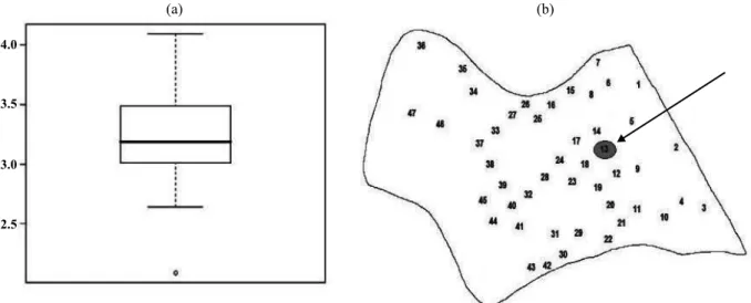
The box-plot graph of soybean yield (Figure 1a), shows an outlier point, with a value of 2.09 t ha-1,
which is the 13th value of the data series, located in
the experimental area (Figure 1b).
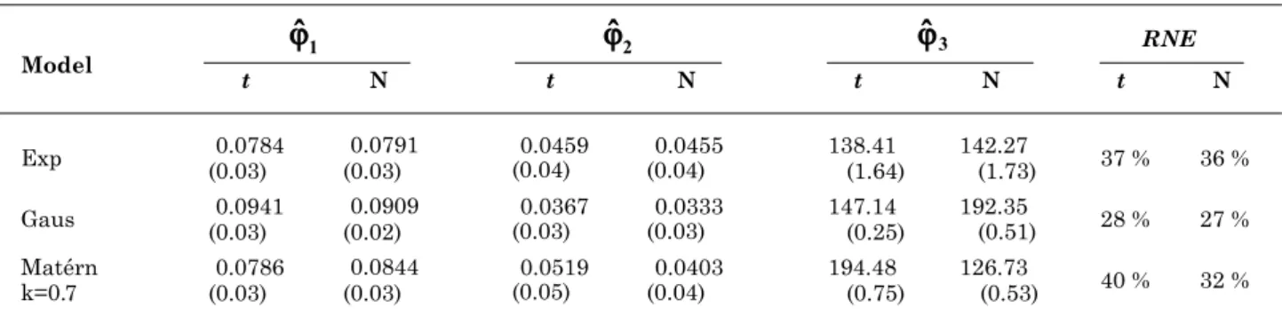
Spatial analysis: Tables 1 and 2 show results of linear spatial model parameter estimates of Equation (10) of soybean yield, setting the following models: exponential (Exp), Gaussian (Gaus), and Matérn with kappa parameter at 0.7. Student’s t-distribution was considered for data with degrees of freedom equal to 3 (v = 3) and normal distribution. The Kolmogorov-Smirnov test was used to confirm the hypothesis that the population distribution, from which the given sample was withdrawn, follows a t-distribution probability with v = 3 degrees of freedom.
Table 2 shows that estimates of parameters (nugget effect), (contribution) and (function of range) have small variations among the three models, assuming Student’s t-distribution with v = 3 or with normal distribution. For both distributions the lowest standard deviation was given by the Gaussian model.
The degree of spatial variability classified by Canarache (1990) by using the coefficient of relative nugget effect (RNE) shows moderate spatial dependence of the variables studied.
Validation of models: Table 3 shows results of the selection criteria for cross-validation models, Akaike information criterion (AIC) and maximum value of the log-likelihood function (LLF) for the soybean yield variate. Considering these results, it
appears that both by the Student’s t-distribution with
v = 3 and by normal distribution, the best-fitting was the Gaussian model.
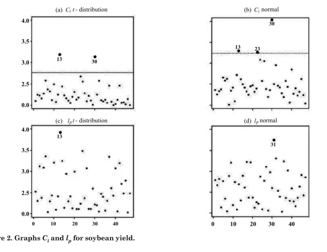
Local Influence Analysis: Graphs Ci in figure 2a,b, considering the limit of the graph defined in Equation (7), shows that by adopting t-distribution with v = 3, elements 13 and 30 are identified as influential for the structure of spatial dependence. However, when adopting normal distribution, elements
Table 1. Parameters estimated by LM assuming Student’s t-distribution with v = 3 and normal for soybean yield using theoretical models: exponential (Exp), Gaussian (Gaus), and Matérn with k = 0.7 (Matérn)
Student’s t-distribution with v = 3, N: normal distribution; In brackets, the standard deviations of each parameter estimated.
Table 2. Parameters estimated when adopting Student’s t-distribution with v = 3 and normal distribution for the yield variable
Student’s t-distribution with v = 3, N: normal distribution; In brackets, the standard deviations of each parameter estimated. EPR(%) = ϕ2/(ϕ1 + ϕ2): coefficient of relative nugget effect.
Table 3. Results of model validation for the soybean yield variate
13, 23, and 30 are identified as influential for the structure of spatial dependence, with greater emphasis on element 30.
According to graphs lp in figure 2c,d, which assess
the influence on the linear predictor, by adopting t -distribution with v = 3, element 13 continues to be considered influential. However, when normal distribution was adopted, element 31 was identified as influential.
Following with the analysis of graphs Ci and lp, it was decided to remove two observations; 13 (2.09 t ha-1)
and 30 (2.87 t ha-1) separately, to identify the influence
of these points in the study of spatial variability. To distinguish the new data sets, we considered Prod: total data, Prod (13): data excluding element 13, and Prod (30): data excluding element 30.
Descriptive analysis after the removal of influential values: Table 4 shows that element 13 produced major changes in the descriptive measures besides the removal of element 30. The removal of these elements also altered data skewness and kurtosis, but according to criteria used to assess normality, new data sets still showed normality.
Parameter vector estimate after the removal of influential values: The parameters were estimated for the three models, for the t -distribution with v = 3 and for the normal distribution, for each one of the variables Prod, Prod (13), and Prod (30). Considering these results, it appears again that both by the t-distribution with v = 3 and by normal distribution, the best-fitting model is the Gaussian model, ie, the removal of influential points did not alter the choice of the set model.
Figure 2. Graphs Ci and lp for soybean yield.
Table 4. Descriptive statistics for the variables Prod, Prod (13) and Prod (30)
n: number of data; Min.: minimum value; Max.: maximum value;
1
Q
: first quartile; Q3: third quartile; S: standard deviation; CV:
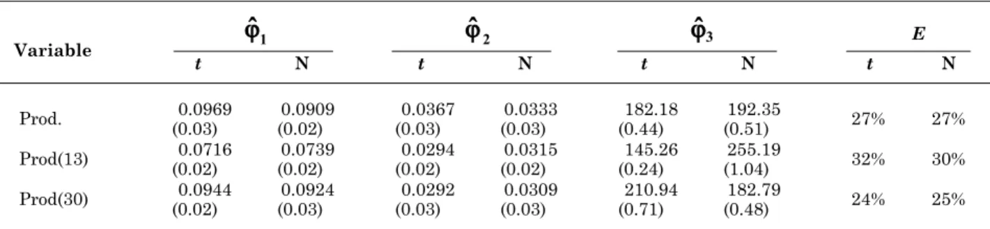
Comparing the estimates of the parameter vector (Table 5) obtained from the data sets Prod (13) and Prod (30), with the estimates obtained with complete data (Prod), it appears that both for the t-distribution (v = 3) and for the normal distribution, estimates 1
and 3 decreased, and estimates 2, 4 and 5
increased. Estimates 6 and 7 have different variations when adopting t-distribution and normal distribution.
Looking at table 6 and considering the t -distribution (v = 3), it appears that changes in the parameters of the structure of spatial variability after the removal of elements 13 (Prod (13)) and 30 (Prod (30)) were the same, showing reduction of the estimates
1 and 2. The estimate 3 was reduced when
obtained with data set Prod (13) and increased when obtained together with the data Prod (30). These changes were more significant for the data set Prod (13) than for Prod (30), when compared to yield (Prod) of the complete data.
However, considering normal distribution, after the removal of element 13 (Prod (13)), there was reduction of 1 and 2 and increase of 3, and after the removal of element 30 (Prod (30)) 1 there was an
increase and the estimates 2 and 3 were reduced. But again these changes were more significant for
data set Prod (13) than for Prod (30), when compared to yield (Prod) of the complete data. Therefore, it can be said that the points identified as influential affect parameter estimates.
When the coefficient of relative nugget effect is examined in the three data sets, it is possible to note that there is no change of the spatial dependence, it remained moderate.
Figure 3 shows the thematic maps of data sets Prod, Prod (13), and Prod (30), based on universal kriging interpolation, using the covariates for the estimation of parameters .
The maps were constructed using the Gaussian model adopting t-distribution (v = 3) and normal distribution. Table 7 shows the percentage of each class on the maps of the variable. From the maps of figure 3 and table 7, it can be observed in figure 3a,b that there was a reduction of the area with yield in the first class interval (2.7 and 3.1 t ha-1) changing
from 35.84 to 31.81 % of the area, and also an increase in areas of the other classes, more pronounced in the 3.1 and 3.3 class t ha-1, from 29.94 to 32.17 %.
Comparing figure 3a,c, it is possible to note a reduction of the area with yield in the interval of the 1st and 4th classes, and increases of the other classes.
Table 5. Parameters estimated when adopting t-distribution with v = 3 and normal for variables Prod, Prod (13), and Prod (30), using Gaussian (Gaus)
Student’s t-distribution with v = 3, N: normal distribution; In brackets, the standard deviations of each parameter estimated.
Table 6. Spatial parameters estimated when adopting t-distribution (v = 3) and normal for variables Prod, Prod (13), and Prod (30), using Gaussian (Gaus)
By comparing figure 3d,e, a reduction in the areas corresponding to the 1st, 2nd and 4th classes is observed,
and an increase in the 3rd class. Comparing figure 3d,f
there is a reduction in the 1st and 3rd, and an increase
in the 2nd and 4th classes. Thus, one can say that the
points identified as influential affect the thematic maps underlying the management of the area with a view to future interventions in the soil treatment. It is therefore important to take all factors into consideration that may alter spatial analysis.
CONCLUSIONS
1. Observation 13 is not only an outlier, but also an influential value. This element (13) had greater influence than element 30 on the estimate of the
Table 7. Percentage of class on the maps of soybean yield
parameters, as well as on the construction of thematic maps, when t-distributions or normal distribution is adopted.
2. In a comparison of the maps, it was noted that the map generated by t-distribution is less changed with the removal of an influential value (13) than the map generated by normal distribution. Therefore, it is possible to perform spatial analysis from Student’s
t-distribution with little concern about influential values, which do not influence this distribution.
ACKNOWLEDGEMENTS
The authors thank the Brazilian Federal Agency for Support and Evaluation of Graduate Education (CAPES), National Council for Scientific and
Technological Development (CNPq) and the Fundação Araucária for financial support.
LITERATURE CITED
BORSSOI, J.A.; URIBE-OPAZO, M.A. & GALEA-ROJAS, M.J. Diagnostic techniques applied in geostatistics for agricultural data analysis. R. Bras. Ci. Solo, 6:1-16, 2009. BORSSOI, J.A.; URIBE-OPAZO, M.A. & GALEA, M. Técnicas de diagnóstico de influência local na análise espacial da produtividade da soja. Eng. Agríc., 31:376-387, 2011. CANARACHE, A.P. A generalized semi-empirical model
estimating soil resistance to penetration. Soil Tillage Res., 16:51-70, 1990.
CHRISTENSEN, R.; JOHNSON, W. & PEARSON, L.M. Prediction diagnostics for spatial linear models. Biometrika, 79:583-591, 1992.
CHRISTENSEN, R.; JOHNSON, W. & PEARSON, L. Covariance function diagnostics for spatial linear models. Intern. Assoc. Mathem. Geol., 25:145-160, 1993. COOK, R.D. Assessment of local influence (with discussion).
J. Royal Stat. Soc., Series B, 48:133-169, 1986.
DEMPSTER, A.; LAIRD, N. & RUBIN, D. Maximum likelihood from incomplete data via the EM algorithm. J. Royal Stat. Soc., Series B, 39:1-38, 1997.
FARACO, M.A.; URIBE-OPAZO, M.A.; SILVA, E.A.; JOHANN J.A. & BORSSOI, J.A. Seleção de modelos de variabilidade espacial para elaboração de mapas temáticos de atributos físicos do solo e produtividade da soja. R. Bras. Ci. Solo, 32:463-476, 2008.
JONES, T. Skewness and kurtosis as criteria of normality in observed frequency distributions. J. Sedim. Res., 39:1622-1627, 1969.
KIEHL, E.J. Manual de edafologia: Relações solo-planta. Piracicaba, Agronômica Ceres, 1979. 264p.
LIU, C. & RUBIN, D.B. ML estimation of the t distribution using EM and its extensions ECM and ECME. Sinica Stat., 5:19-39, 1995.
MILITINO, A.F.; PALACIOS, M.B. & UGARTE, M.D. Outlier detection in multivariate spatial linear models. J. Stat. Planning Infer., 136:125-146, 2006.
MOLIN, J.P. Definição de unidades de manejo a partir de mapas de produtividade. Eng. Agríc., 22:83-92, 2002. PAULA, G.A. Modelos de regressão com apoio computacional.
São Paulo, Instituto de Matemática e Estatística – USP, 2004. 233p.
POON, W.Y. & POON, Y.S. Conformal normal curvature and assessment of local influence. J. Royal Stat. Soc.. Series B (Statistical Methodology), 61:51-61, 1999.
R DEVELOPMENT CORE TEAM. R: A language and environment for statistical computing. R Foundation Stat. Computing, ISBN 3-900051-07-0. Available at: <http:// www.R-project.org>. Accessed June 3, 2009.
RIBEIRO JR., P.J. & DIGGLE P.J. geoR: A package for geostatistical analysis. R-NEWS, 01. Available at <http:// cran.r-project.org/doc/Rnews. 2001>. Accessed June 3, 2009.
ROWLINGSON, B. & DIGGLE, P.J. Splancs: Spatial point pattern analysis code in S-Plus. Comp. Geosci., 19:627-655, 1993.