Procedures for finite element mesh generation from medical imaging: application to the intervertebral disc

(1)

(2)

ii

DECLARAÇÃO

Nome: Sara Isabel Couto Cortez

Endereço eletrónico: a49951@alunos.uminho.pt Telefone: 00351 964 747 658 Número do Bilhete de Identidade: 13399554

Título da dissertação: Procedures for Finite Element Mesh Generation from Medical Imaging. Application to the Intervertebral Disc.

Ano de conclusão: 2011

Orientador: Professor Doutor José Luis Carvalho Martins Alves

Designação do Mestrado: Ciclo de Estudos Integrados Conducentes ao Grau de Mestre em Engenharia Biomédica

Área de Especialização: Biomateriais, Reabilitação e Biomecânica Escola: de Engenharia

Departamento: de Engenharia Mecânica

DE ACORDO COM A LEGISLAÇÃO EM VIGOR, NÃO É PERMITIDA A REPRODUÇÃO DE QUALQUER PARTE DESTA TESE/TRABALHO.

Guimarães, ____/____/________

(3)

iii

Acknowledgments

Firstly, I would like to thank my mentor Professor José Luis Alves, for his availability, knowledge, experience, constant support, timely guidance and suggestions throughout this project. His words made me grow professionally.

I am grateful to Professor J.C. Pimenta Claro for his support.

I would also like to express my sincere gratitude to Manuel Pinheiro, for all the support and encouragement throughout this work.

I gratefully acknowledge the support of the European Project: NP Mimetic - Biomimetic Nano-Fiber Based Nucleus Pulposus Regeneration for the Treatment of Degenerative Disc Disease,

funded by the European Commission under FP7 (grant NMP3-SL-2010-246351).

I am grateful to CT2M - Centre for Mechanical and Materials Technologies, to Mechanical Engineering Department and to University of Minho, as well as to all their collaborators, for sponsoring my research and providing an excellent work environment.

I would like to thank all my friends, especially to Sara Tribuzi, Maria Martins and Ravi Patel for their unconditional help.

Finally, I would like to thank to my parents, my brother and Diogo for their continued support and guidance and for believing in my capabilities.

(4)

(5)

v

Abstract

Procedures for Finite Element Mesh Generation from Medical Imaging. Application to the Intervertebral Disc.

The paramount goal of this ‘half-year’ work is the development of a set of methodologies and procedures for the geometric modelling by a finite element (FE) mesh of the bio-structure of a motion segment (or functional spinal unit), i.e., two vertebrae and an intervertebral disc, from segmented medical images (processed from medical imaging).

At an initial stage, a three-dimensional voxel-based geometric model of a goat motion segment was created from magnetic resonance imaging (MRI) data. An imaging processing software (ScanIP/Simplewire) was used for imaging segmentation (identification of different structures and tissues), both in images with lower (normal MRI) and higher (micro-MRI) resolutions. It shall be noticed that some soft-tissues, such as annulus fibrosus or nucleus pulposus, are very hard to isolate and identify given that the interface between them is not clearly defined. At the end of this stage, images with different resolutions allowed to generate different 3D voxel-based geometric models.

Thereafter, a procedure for the FE mesh generation from the aforementioned voxelized data should be studied and applied. However, as the original geometry was only approximately known from real medical imaging, it was difficult to objectively quantify the quality of the FE meshing procedure and the accuracy between source geometry and target FE mesh. In order to overcome such difficulties, and due to the lack of quality of the available medical imaging, a “virtualization” procedure was developed to create a set of segmented 2D medical images from a well-defined geometry of a motion segment. The main idea was to create the conditions to quantify the quality and the accuracy of the developed FE meshing procedure, as well to study the effect of imaging resolution.

Starting from the virtually generated 2D segmented images, a 3D voxel-based structure was achieved. Given that initial domains are now clearly defined, there is no need for further image processing. Then, a two-step FE mesh generation procedure (generation followed by simplification) allows to create an optimized tetrahedral FE mesh directly from 3D voxelized data. Finally, because the virtualization procedure allowed to know the initial geometry, one is able to objectively quantify

(6)

vi

the quality and the accuracy of the final simplified tetrahedral FE mesh, and thus to understand and quantify: a) the role of the medical image resolution on the FE geometrical reconstruction, b) the procedure and parameters of the FE mesh generation step, and c) the procedure and parameters of the FE mesh simplification step, and thus to give a clear contribution in the definition of the procedure for the FE mesh generation from medical imaging in case of an intervertebral disc.

(7)

vii

Resumo

Procedimentos de Geração de Malha de Elementos Finitos a partir de Imagem Médica. Aplicação ao Disco Intervertebral.

O objetivo fundamental deste trabalho de seis meses é o desenvolvimento de um conjunto de metodologias e procedimentos para a modelação geométrica, através de uma malha de elementos finitos (EF) de uma bio-estrutura de um motion segment (ou unidade funcional da

coluna), ou seja, duas vértebras e um disco intervertebral, a partir de imagens médicas segmentadas (processadas a partir de imagiologia médica).

Numa fase inicial, um modelo geométrico tridimensional baseado em voxels de um motion segment de uma cabra foi criado a partir de informação de imagens médicas de ressonância

magnética (RM). Um software de processamento de imagem (ScanIp/Simplewire) foi usado para

segmentação de imagens (identificação de diferentes estruturas e tecidos), em imagens de menor (RM normal) e maior (micro-RM) resolução. Deve ser referido que alguns tecidos moles, como o anel fibroso e o núcleo pulposo são muito difíceis de isolar e identificar, dado que as fronteiras destes não estão claramente definidas. No final desta etapa, as imagens com diferentes resoluções permitiram gerar diferentes modelos geométricos 3D baseados em voxels.

Posteriormente, um procedimento para geração de malha de EF, a partir da informação voxelizada acima mencionada, deveria ser estudado e aplicado. No entanto, como a geometria original era aproximadamente conhecida a partir de imagens médicas reais, foi difícil quantificar objetivamente a qualidade do procedimento de geração de malha de EF e a precisão entre a geometria de origem e a malha de EF de destino. A fim de superar tais dificuldades, e devido à falta de qualidade de imagens médicas disponíveis, um procedimento de “virtualização” foi desenvolvido para criar um conjunto de imagens médicas 2D segmentadas a partir de uma geometria de um motion segment bem conhecida. A principal ideia foi criar as condições para

quantificar a qualidade e a precisão do procedimento de geração de malha de EF desenvolvido, bem como estudar o efeito da resolução da imagem médica.

A partir das imagens 2D segmentadas, geradas virtualmente, uma estrutura de voxels 3D pode ser conseguida. Dado que os domínios iniciais estão agora claramente definidos, não há necessidade de processamento de imagem adicional. Por conseguinte, um procedimento de

(8)

viii

geração de malha de EF de duas etapas (geração seguida por simplificação) permite criar uma malha de EF tetraédrica otimizada diretamente a partir de informação 3D voxelizada.

Por fim, como o procedimento de virtualização permitiu conhecer a geometria inicial, é possível quantificar objetivamente a qualidade e exatidão da malha de EF tetraédrica final simplificada, e assim, compreender e quantificar: a) o papel da resolução da imagem médica na reconstrução geométrica de EF; b) o procedimento e os parâmetros da etapa de geração de malha de EF; c) o procedimento e os parâmetros da etapa de simplificação de malhas de EF, e assim, dar uma contribuição clara na definição do procedimento para a geração de malha de EF a partir de imagem médica, no caso de um disco intervertebral.

(9)

ix

Acronyms

2D – two-dimensional 3D – three-dimensional AF – annulus fibrosus

BCC – body-centred cubic lattice CEP – cartilaginous endplate CT – X-ray computed tomography

DICOM - Digital Imaging and Communications in Medicine DDD – degenerative disc disease

FE – finite element

FEA – finite element analysis FOV – field of view

HU – Hounsfield units IVD – intervertebral disc NP – nucleus pulposus

MRI – magnetic resonance image ROI – region of interest

(12)

(13)

xiii

List of Figures

Figure 2.1 – The Human spine... 9 Figure 2.2 – The vertebral structure [Daavittila, 2007]. ... 10 Figure 2.3 – The motion segment consisting of two vertebral bodies and a normal IVD between

them [adapted from [Raj, 2008]. ... 12 Figure 2.4 - The components of the intervertebral disc (adapted from [Postacchini, 1999])... 12 Figure 2.5 – Mid-sagittal sections of intervertebral discs showing the biochemical appearance of

ageing (A) a disc typical of ages 20–30 years and (B) a disc typical of ages 50–60 years [Adams et al., 2010]. ... 15

Figure 2.6 – Compression loading (A) a normal non-degenerated and (C) degenerated disc. Outer annulus layers have a large tension stress along the fibres and also in the tangential peripheral direction. The inner annulus fibres have stresses of smaller magnitude (B). Annulus fibres show outer layers are subjected to increased amount of tensile stress. The inner annulus fibres have a high compressive stress (D) [Jensen, 1980]. ... 15 Figure 3.1 – Plain radiographs showing the following: (A) Narrowing of the L5-S1 disc space with

mild osteophyte formation demonstrating mild DDD at this single level. (B) Disc space narrowing, endplate sclerosis, and osteophytes at L1-L2, L2-L3, L4-L5, and L5-S1 in this patient with marked multi-level DDD. Retrolisthesis of L3 on L4 is also seen [Wills et al., 2007]. ... 18

Figure 3.2 – Principle of the plain radiography technique (adapted from [Butler et al., 2007]) ... 18

Figure 3.3 – CT scan showing complete loss of the L5-S1 disc space with severe endplate sclerosis and development of osteophytes. [Wills et al., 2007]. ... 19

Figure 3.4 – Principle of different generations of CT scanner. First (A), Second (B), Third (C), Fourth (D) and modern (E) generation scanner (adapted from [Zeng, 2010]). ... 20 Figure 3.5 – The principle of attenuation. ... 21 Figure 3.6 – The tiny bar magnets (A) before and (B) after the tissues being placed within a strong

magnetic field. ... 23 Figure 3.7 – T1-weighted (A) and T2-weighted (B) sagittal MRI demonstrating a disc herniation at

L4-L5 [Wills et al., 2007]. ... 23

Figure 4.1– The pixel and the voxel representation. ... 28 Figure 4.2 – The three main imaging plans of the human body: sagittal (YZ), coronal (XZ) and axial

(14)

xiv

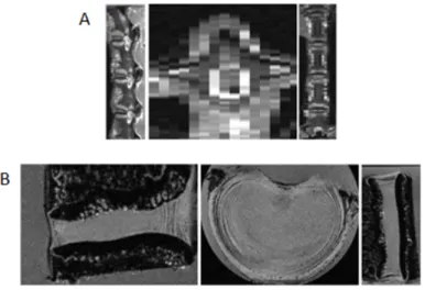
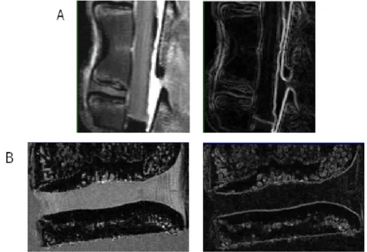
Figure 4.3 – The (A) MR and (B) micro-MR images of the lumbar goat motion segment in different

planes (sagittal, axial and coronal, respectively). ... 29

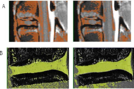
Figure 4.4 – The thresholding algorithm applied to the (A) MR and (B) micro-MR images. ... 33

Figure 4.5 – The gradient magnitude filter applied to the (A) MR and (B) micro-MR images. ... 34

Figure 4.6 – The Canny Operator applied to the (A) MR and (B) micro-MR images after thresholding. ... 35

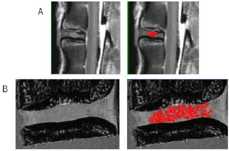
Figure 4.7 – The region growing algorithm applied to the (A) MR and (B) micro-MR images. ... 36

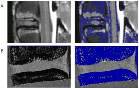
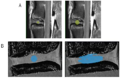
Figure 4.8 – The segmentation of the IVD with the geodesic active contour applied to the (A) MR and (B) micro-MR images. ... 39

Figure 4.9 – Two different 3D models based on (A) 0.3x0.3x3.3 mm3 and (B) 0.12x0.12x0.12 mm3 of MR image resolution. ... 39

Figure 4.10 – Two examples of micro-MR images of the IVD converted into colour images... 40

Figure 4.11 – Data flow diagram of the segmentation procedure applied to a motion segment based on micro-MR images. ... 41

Figure 5.1 – Reference FE mesh of the human lumbar motion segment (from the ISB Finite Element Repository). ... 45

Figure 5.2 - – A two-dimensional illustration of the (three-dimensional) creation of the grid of pixels (voxels). ... 46

Figure 5.3 – Schematic representation of the equivalence between Cartesian and canonical spaces of a given finite element. ... 47

Figure 5.4 – Example of a 8-node hexahedron drawn in the canonical frame. ... 47

Figure 5.5 – Schematic of the virtual segmentation process on the pixels matrix. ... 49

Figure 5.6 – Schematic of three different dimensions of pixels. ... 50

Figure 5.7 – Sagittal sectioning (X=2) of the motion segment with a) 0.3x0.3x3.3 b) 0.12x0.12x0.12 and c) 0.3x0.3x0.3 mm3 of the voxel size. ... 52

Figure 5.8 - Coronal sectioning (Y=2) of the motion segment with a) 0.3x0.3x3.3 b) 0.12x0.12x0.12 and c) 0.3x0.3x0.3 mm3 of the voxel size. ... 53

Figure 5.9 - Axial sectioning (Z= -5) of the motion segment with a) 0.3x0.3x3.3 b) 0.12x0.12x0.12 and c) 0.3x0.3x0.3 mm3 of the voxel size. ... 54

Figure 5.10 - Axial sectioning (Z=0) of the motion segment with a) 0.3x0.3x3.3 b) 0.12x0.12x0.12 and c) 0.3x0.3x0.3 mm3 of the voxel size. ... 55

(15)

xv Figure 5.12 – A two-dimensional illustration of the (three-dimensional) FE mesh generation algorithm. ... 60 Figure 5.13 – Sagittal cross section (X=2.0 mm) of the initial geometry (coloured domains) and

the contour of the FE mesh for the resolution of 0.3x0.3x3.3 mm3. The parameters used were a grid size of 2.0 mm (and N of 1.04) and σ of a) 0.52 b) 1.04 c) 2.08. ... 62 Figure 5.14 - Sagittal cross section (X=2.0 mm) of the initial geometry (coloured domains) and the

contour of the FE mesh for the resolution of 0.12x0.12x0.12 mm3. The parameters used were a grid size of 2.0 mm (and N of 16.67) and σ of a) 8.33 b) 16.67 c) 33.33. ... 63 Figure 5.15 – Sagittal cross section (X=2.0 mm) of the initial geometry (coloured domains) and

the contour of the FE mesh for the resolution of 0.3x0.3x0.3 mm3. The parameters used were a grid size of 2.0 mm (and N of 6.67) and σ of a) 3.33 b) 6.67 c) 13.33... 64 Figure 5.16 – Sagittal cross section (X=2.0 mm) of the initial geometry (coloured domains) and

the contour of the FE mesh for the resolution of 0.3x0.3x3.3 mm3. The parameters used were a grid size of 1.0 mm (and N of 0.52) and σ of a) 0.26 b) 0.52 c) 1.04. ... 65 Figure 5.17 - Sagittal cross section (X=2.0 mm) of the initial geometry (coloured domains) and the

contour of the FE mesh for the resolution of 0.12x0.12x0.12 mm3. The parameters used were a grid size of 1.0 mm (and N of 8.33) and σ of a) 4.17 b) 8.33 c) 16.67... 66 Figure 5.18 – Sagittal cross section (X=2.0 mm) of the initial geometry (coloured domains) and

the contour of the FE mesh for the resolution of 0.3x0.3x0.3 mm3. The parameters used were a grid size of 1.0 mm (and N of 3.33) and σ of a) 1.67 b) 3.33 c) 6.67. ... 67 Figure 5.19 – Sagittal cross section (X=2.0 mm) of the initial geometry (coloured domains) and

the contour of the FE mesh for the resolution of 0.3x0.3x0.3 mm3. The parameters used were a grid size of 0.5 mm (and N of 0.26) and σ of a) 0.26 b) 0.52. ... 68 Figure 5.20 – Sagittal cross section (X=2.0 mm) of the initial geometry (coloured domains) and

the contour of the FE mesh for the resolution of 0.12x0.12x0.12 mm3. The parameters used were a grid size of 0.5 mm (and N of 4.17) and σ of a) 2.08 b) 4.17 c) 8.33. ... 69 Figure 5.21 – Sagittal cross section (X=2.0 mm) of the initial geometry (coloured domains) and

the contour of the FE mesh for the resolution of 0.3x0.3x0.3 mm3. The parameters used were a grid size of 0.5 mm (and N of 1.67) and σ of a) 0.83 b) 1.67 c) 3.33. ... 70 Figure 5.22 – FE mesh obtained for the resolution of 0.3x0.3x3.3 mm3, grid size of 0.5 mm and σ

(16)

xvi

Figure 5.23 - FE mesh obtained for the resolution of 0.12x0.12x0.12 mm3, grid size of 0.5 mm and σ value of 8.33. ... 74 Figure 5.24 - FE mesh obtained for the resolution of 0.3x0.3x0.3 mm3, grid size of 0.5 mm and σ

value of 3.33. ... 74 Figure 6.1 – FE mesh simplification by edge contraction. ... 79 Figure 6.2 - Sagittal sectioning (X=2) of the FE mesh based on the resolution of 0.12x0.12x0.12

mm3 for a) simplification 1: 100 000; b) simplification 2: t0.05] 100 000; c) simplification 3: [-t0.05] [-g] 100 000. ... 82 Figure 6.3 - Sagittal sectioning (X=2) of the FE mesh based on the resolution of 0.3x0.3x0.3 mm3 for a) simplification 1: 100 000; b) simplification 2: t0.05] 100 000; c) simplification 3: [-t0.05] [-g] 100 000. ... 83 Figure 6.4 - FE mesh obtained based on simplification 2 from voxel size of 0.12x0.12x0.12 mm3 with sizing parameters of (left) 0.5 and 10 (right) 1.0 and 10 for max edge length inside the IVD and max edge length outside the IVD, respectively. ... 86 Figure 6.5 - FE mesh obtained based on simplification 2 from voxel size of 0.3x0.3x0.3 mm3 with

sizing parameters of (left) 0.5 and 10 (right) 1.0 and 10 for max edge length inside the IVD and max edge length outside the IVD, respectively. ... 86 Figure 6.6 - Sagittal sectioning (X=2) of the FE mesh based on simplification 2 from voxel size of

0.12x0.12x0.12 mm3 for a) 0.5 and 10 b) 1.0 and 10 of the edge length in IVD and edge length outside of the IVD, respectively. ... 87 Figure 6.7 –Sagittal sectioning (X=2) of the FE mesh based on simplification 2 from voxel size of

0.3x0.3x0.3 mm3 for a) 0.5 and 10 b) 1.0 and 10 of the edge length. ... 88 Figure 6.8 – Meshes from simplification with relative sizing of 1:20 (upper mesh) and 1:10 (lower

mesh). ... 90 Figure 7.1 - Proposed FE mesh generation procedure developed in this study. ... 93 Figure 8.1 – Characterization of the porcine lumbar motion segment using a destructive serial-sectioning technique... 95 Figure A.1 - A geometric interpretation of the Newton-Raphson method. ... 101

(17)

xvii

List of Tables

Table 1.1 – Summary of the most relevant publications about FE mesh generation of a motion segment. ... 2 Table 3.1 – Resolution and some characteristics of images from different medical imaging

techniques. ... 25 Table 4.1 – Comparison between the two types of MRI images used in this work. ... 30 Table 5.1 – Three different resolutions (voxel’s dimension) of the voxel used in this study. ... 50 Table 5.2 – Number of elements and volumes of the voxel and the initial geometry of different

materials with 0.3x0.3x3.3 mm3 of the voxel dimension. ... 56 Table 5.3 - Number of elements and volumes of the voxel and the initial geometry of different

materials with 0.12x0.12x0.12 mm3 of the voxel dimension. ... 56 Table 5.4 - Number of elements and volumes of the voxl and the initial mesh for different materials

with 0.3x0.3x0.3 mm3 of the voxel dimension. ... 56 Table 5.5 – Different parameters used in FE mesh generation. ... 58 Table 5.6 – Volumes of the different materials of the generated FE meshes with a voxel dimension

of 0.3x0.3x3.3 mm3. ... 71 Table 5.7 – Volumes of the different materials of the final FE mesh with a voxel dimension of

0.12x0.12x0.12 mm3. ... 72 Table 5.8 – Volumes of the different materials of the final FE mesh with a voxel dimension of

0.3x0.3x0.3 mm3. ... 73 Table 6.1 – Description of the different refinement criteria of the mesh simplification procedures. ... 80 Table 6.2 – Simplification case studies. ... 81 Table 6.3 – Number of nodes and elements and the dihedral angles for different simplification

tests. ... 84 Table 6.4 – Sizing tests performed with absolute parameter. ... 85 Table 6.5 - Number of elements and nodes and the dihedral angles for different simplification tests

with two different edges length. ... 88 Table 6.6 – Sizing tests performed with relative parameter for a non-simplified mesh. ... 89

(18)

(19)

Chapter 1. Introduction

1.1. Motivation and Scope

The Degenerative Disc Diseases (DDD) is a relatively common problem of the spine, particularly in the lumbar region [Rannou et al., 2001]. The low back pain is an important disease pertaining to

human health as it may limit mobility and affect normal functions of the spine. Its incidence tends to increase every year and to affect a large portion of the population [Urban et al., 2003].

Biomechanics and several biomechanical tests and studies have given essential contributions to find the causes and solutions for this problem.

The Finite Element Analysis (FEA) is an essential tool to study the behaviour of the spine, especially to investigate the bio-mechanisms of the intervertebral disc (IVD). The benefits of using FEA in biomechanical studies are obvious and this method has definitely contributed to improve our understanding on the biomechanics of the spine. In most cases biological structures are not easy to study in vivo, and only computational models and numerical simulations are easily

accessible allowing to have an “inside” view. IVDs are no exception, as they are hardly accessible. Around the world, research groups have devoted attention to this subject and have applied FE modelling to study the biomechanics of the IVD.

Virtual 3D models, such as 3D FE meshed, can be used to “virtualize” the internal structures of the Human body, and thus contributing to medical diagnosis of pathologies; to decide rehabilitation strategies; to virtualize surgeries and a priori evaluation of surgical strategies.

However, the 3D reconstruction process of a patient-oriented data is somewhat tricky and is known to have some problems that cause a number of difficulties in the FE analysis, such as the identification of tiny or too complex geometric details. The accuracy of the FE computation increases if the geometry of model resembles the real structure.

In general, a FE model can be created from a solid voxel-based 3D model obtained from 3D reconstruction of a set of 2D medical images. Medical images are usually obtained from any

(20)

medical imaging technique, such as radiography, X-Ray Computer Tomography (CT), Magnetic Resonance Imaging (MRI), or other. In fact, most of these models are based on CT images, MRI images or a combination of CT and MRI images and some of them are even created by algorithms using “standard” dimensions mentioned in literature [Tyndyka et al., 2007]. Table 1.1 shows some

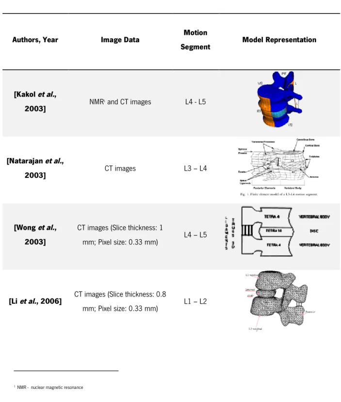
of the most relevant 3D models of a motion segment based on different protocols and data, as was found in literature.

Table 1.1 – Summary of the most relevant publications about FE mesh generation of a motion segment.

Authors, Year Image Data Motion

Segment Model Representation

[Kakol et al., 2003] NMR 1 and CT images L4 - L5 [Natarajan et al., 2003] CT images L3 – L4 [Wong et al., 2003]

CT images (Slice thickness: 1

mm; Pixel size: 0.33 mm) L4 – L5

[Li et al., 2006] CT images (Slice thickness: 0.8

mm; Pixel size: 0.33 mm) L1 – L2

(21)

(continued) Table 1.1 - The studies of the 3D motion segment models.

[Zhong et al.,

2006] CT images L1 – L3

[Schmidt et al., 2007]

CT images (Slice thickness: 0.75 mm; Pixel size: 0.49 mm) and

MRI images L4 –L5 [Renner et al., 2007] CT images L1 –S1 [Natarajan et al., 2007] CT images L4 – L5 [Meng et al., 2009]

CT images (Slice thickness: 1

mm) L4 – L5

[Swider et al.,

2010] MRI images L5 – S1

[Bao et al., 2010]

CT images (Slice thickness: 0.75

(22)

Despite all 3D models are based on specific and real data (essentially CT), significantly different geometries can be seen. Such big differences when dealing with similar real structures reveal basically the lack of robustness of the 3D reconstruction process, and not simply real differences on medical images and/or anatomical information and histological observations. However, it is also known that both the type of medical imaging technique and image resolution have a key role in the 3D reconstruction process. Sometimes these geometrically-based models do not provide complete information about the different structures due to the low resolution of most medical images, i.e., very tiny details and tiny structures are very probably lost “inside” resolution. On the other hand, some soft tissues of IVD, especially nucleus pulposus and annulus fibrosus, have similar density and constitution, what makes 3D reconstruction even more difficult and imaging segmentation a very user-dependent task. CT images has proved to be a good tool to aid in the segmentation of bone structures but turned out to be less efficient than MRI images in the detection of soft tissues such as the ones in the intervertebral disc.

The resolution of medical images, i.e., pixel size and slice thickness, plays also an important role in the accuracy of 3D geometrical reconstruction of anatomical structures from 2D images, and consequently of final FE meshes. Resolution provides information regarding which technique can or shall not be used for 3D reconstruction. The aim of this work is to establish an optimized procedure for the generation of a 3D FE mesh of a motion segment in general, and an intervertebral disc in particular, in order to allow the development of new biomechanical simulations of intervertebral discs. It will be shown that the original imaging resolution plays a paramount role on the quality and accuracy of the generated FE meshes. Besides, such requirements for the biomechanical studies can drive the specifications for future improved medical imaging equipments.

Although a multi-segment FE model have many advantages and have contributed significantly to quantify the biomechanics of the spine, in this work, a motion segment (L4 – L5) FE mesh originally created by T.H. Smit (available on the web from the ISB Finite Element Repository2) was re-worked and used as a reference geometry to allow an objective comparison with the final FE meshes obtained from the newly proposed FE mesh generation procedure.

(23)

1.2. Aim

The paramount goal of this study is the development of a set of methodologies and procedures for the 3D geometrical/anatomical modelling by a finite element mesh of the bio-structure of a motion segment, i.e., two vertebrae and an intervertebral disc, from images acquired by any medical imaging technique. A simplified and optimized finite element mesh must be generated in order to couple the patient-oriented data acquisition from medical imaging with computational FEA of the biomechanics of the human spine.

To investigate the influence of medical imaging resolution on the final quality of the generated geometric model by finite elements, an algorithm for the generation of a set of 2D virtual and segmented medical images is developed and implemented. Then, a procedure allowing the generation of a tetrahedral FE mesh from 3D reconstructed and segmented medical imaging is applied. The main purpose behind the abovementioned idea is to allow establishing some objective criteria for the evaluation and quantification of the impact of the reconstruction parameters and FE mesh generation procedure by comparing objectively the final geometrical reconstruction by finite elements and the well-defined and initial geometry of a lumbar motion segment, in order to understand the role of the medical image resolution and FE mesh generation procedure and parameters on the geometrical reconstruction by finite elements from medical imaging data.

In summary, once the 2D image scanning data of an intervertebral motion segment are obtained, one shall be able to:

a) produce a 3D voxel-based model from the 2D medical images;

b) study the influence of the medical imaging parameters (resolution, segmentation, etc.) over the FE meshing technique of a lumbar motion segment;

c) generate a good quality and optimized finite element mesh, with a special emphasis on an accurate modelling of the biological and anatomical features and surrounding tissues and bones of a motion segment in general, and the intervertebral disc in particular.

This study is framed under an on-going European project denominated “NPmimetic - Biomimetic Nano-Fibre-Based Nucleus Pulposus Regeneration for the Treatment of Degenerative Disc Disease”, which seeks to develop a biomimetic strategy for the IVD

regeneration. Under this framework, the primary goal of the present study is to develop a procedure to obtain a simplified and optimized FE mesh describing geometrically a patient-oriented

(24)

intervertebral motion segment based on medical images, which can be used for future computational analysis of the biomechanics of the IVD, numerical analysis of the rehabilitation procedures and specification of the mimetic materials to be developed.

1.3. Limitation of the study

The primary idea behind this work was to use real medical imaging data, which should be processed and segmented in order to allow a 3D geometrical reconstruction. These 3D voxel-based geometric models should be hereafter used for the FE mesh generation in order to obtain the final 3D geometrical reconstruction by finite elements. However, some obstacles appeared along this way, which made mandatory to update the initially proposed flowchart. In brief, the most common problems were the lack of resolution of the medical images, the ambiguous definition of tissues' boundaries, what made difficult to isolate and identify soft tissues like annulus fibrosus or nucleus pulposus and thus to attain a reliable segmentation, and a clear and unambiguous identification of the reference geometry for comparison purposes. On the other hand, for very low resolution images it was hard to define the boundaries between two different anatomic regions with a similar density and constitution, and any user-decision could drive to a non-negligible variation of the initial geometry. Real images were not used to study the influence of resolution on the FE mesh generation procedure.

1.4. Organization of thesis

Chapter 1 briefly presents the main framework of this thesis, main problems of the spine, the motivation, aims and some limitations faced during the development of this work.

Chapter 2 gives a brief description of the main features of the Human spine system and its constituents (in particular the IVD). It also provides a brief description of the biomechanics of the IVD and related degenerative disc diseases.

The main medical imaging techniques are briefly presented in Chapter 3. Only the most relevant techniques used in the diagnostic of degenerative diseases of the lumbar spine are detailed, such as plain radiography, computed tomography (CT), magnetic resonance imaging (MRI), micro-CT and micro-MRI.

(25)

2D medical images, are the starting point for FE mesh generation procedures. Thus, this Chapter addresses several questions such as 2D image properties, segmentation algorithms used for image processing and procedures for generation of the 3D voxel-based geometric model. The image resolution and its influence on accuracy geometric model are also discussed in this Chapter, and illustrated with the 3D reconstruction of a goat IVD from real medical imaging data.

In Chapter 5 the procedure for the FE mesh generation from 3D voxel-based geometric models is discussed. An algorithm for the construction of a set of virtual and segmented 2D images is introduced and described. Finally, the influence of each parameter of the mesh generation procedure on the final FE mesh is presented and discussed.

Chapter 6 presents a comparison between final geometry described by the optimized and simplified FE mesh and the initial geometry of the motion segment. Such comparison allows the definition of several quality criteria to classify the FE mesh generation procedure.

Finally, main conclusions and FE mesh generation guidelines are drawn in Chapter 7 whereas future work, which is already in development, is covered in chapter 8.

(26)

(27)

Chapter 2. The Human spine system

2.1. Anatomy

The Human spine (or vertebral column) has some important functions such as: to provide the body structural support, to protect the spinal cord, nerve roots, and many internal organs, to enable trunk movements (e.g., flexion, extension, lateral bending, and axial rotation). These spine capabilities depend essentially of its constitution [Niosi et al., 2004; Jongeneelen, 2006; Shankar et al., 2009].

Figure 2.1 – The Human spine.

The spine is fundamentally composed of vertebral bodies and intervertebral discs. It extends from the base of the skull, passes through the neck, trunk and goes all the way to the

(28)

pelvis (Figure 2.1). The spine consists of 33 separated vertebrae: five of them are sacral vertebrae, which are fused to form the sacrum, and four are coccygeal vertebrae, which are fused to form the coccyx. In adult persons, there are 24 motion segments named according to their location in the intact column, seven cervical (C1 to C7), twelve thoracic (T1 to T12), five lumbar (L1 to L5) and ending with the sacral vertebrae (S1 to S5). One motion segment is composed of two vertebral bodies and one disc. The surfaces of the vertebral body are enclosed by a thin layer of hyaline cartilage, called endplates, and the nutrition of the intervertebral discs is done through these structures by diffusion process [Naegel, 2007; Shankar et al., 2009].

The vertebra size varies along in spine, cervical being the smallest and lumbar the largest. Nevertheless, the basic structure of the vertebral body remains the same. Each vertebra consists of an anterior vertebral body and a posterior arch. The body is the thick zone of the vertebra composed of spongy medullary bone surrounded by a dense bony cortex. The neural arch has a pair of pedicles on its sides and two laminae. The laminae are broad flat plates of bone that are extended from the pedicles and, when they fuse with the lamina of the vertebra below, form the roof of the vertebral foramen, thus forming a canal to protect the spinal cord [Daavittila, 2007]. The vertebral arch also supports one spinous, two transverse and four articular processes. A spinous process is typically palpable through the skin. Superior and inferior articular facets on each vertebra act to restrict the vertebral column movement. Figure 2.2 shows the constitution of one vertebra.

(29)

Furthermore, the vertebrae are also connected to each other by paired facet joints between the articular processes and by strong anterior and posterior longitudinal ligaments, which extend the length of the whole vertebral column and are attached to the intervertebral discs and vertebral bodies.

The anterior longitudinal ligament is a strong, broad fibrous band covering and connecting the anterior features of the vertebral bodies and intervertebral discs. Their fibres are firmly bound to the surface of the intervertebral discs, and the periosteum of the vertebral bodies is thickest on the front side of the discs. The posterior longitudinal ligament runs along the posterior side of the vertebral column within the vertebral canal. It has a characteristic appearance with extensions over to intervertebral discs, narrowing as it passes each vertebral body. The posterior longitudinal ligament narrows down caudally. Additionally, the flavum, supraspinous and interspinous ligaments can also help to stabilize the spine [Ebraheim et al., 2004].

2.2. Intervertebral disc

The intervertebral disc is a cartilaginous structure that contributes to flexibility and weight support in the spine. The IVDs are the most important structural links between adjacent vertebrae. They are exposed to a considerable variety of mechanical loadings (forces and moments), such as compressive loads arising from body weight and muscle activation, and connect one vertebral body to the next one [Urban et al., 2000].

There are 23 intervertebral discs along the whole spine, and their heights differ between vertebrae (approximately 8-10 mm in height and 4 cm in diameter). In young persons, the IVDs between the bodies of sacral and coccygeal vertebrae are present but will eventually disappear while ageing [Raj, 2008]. Additionally, the IVD’s height comprises approximately 25% of the total height of the vertebral column. The different curvatures of the spine, particularly in the cervical and lumbar region, are associated with the different height of the intervertebral disc (Figure 2.3). In the cervical region, the IVD geometry tends to be oval, while in the thoracic region it resembles a heart-like and in the lumbar region it looks like a kidney.

(30)

Figure 2.3 – The motion segment consisting of two vertebral bodies and a normal IVD between them [adapted from [Raj, 2008].

Each IVD is composed of an outer laminated and densely annulus fibrosus surrounding an inner gelatinous nucleus pulposus. Its structure is located between the cartilaginous endplates of the vertebrae as shown in the Figure 2.4. An apparent boundary between nucleus pulposus and annulus fibrosus can be identified in this image. The intervertebral disc has its own unique structural and metabolic properties. Its composition changes significantly during development, growth, ageing and degeneration, what changes the way how discs respond to changes in mechanical loadings [Adams et al., 2010]. Recently, with the development of magnetic resonance

imaging (MRI) techniques, the nutrition supply of the IVD has been investigated in vivo in animals

and humans [Haughton, 2006]. It has been suggested that the loss of nutrient supplies may lead to disc degeneration.

(31)

2.2.1. Nucleus Pulposus

The nucleus pulposus (NP) is the soft and hydrophilic part of the IVD and it is located within the central zone of the disc (Figure 2.4). The NP contains fibrocytes as well as chondrocytes, and an isotropic tissue based on fibres organized randomly and arranged radially. The fibres are substantially collagen and elastin fibres, which may be more than 150 µm in length. They are embedded in a highly hydrated proteoglycan-water gel. The role of the proteoglycan is to attract water and to give the nucleus its swelling capacity, and thus developing an osmotic pressure. Its extracellular matrix is gelatinous and the cells of the NP are originally derived from the notochord [Raj, 2008]. The boundary between nucleus and annulus is not well defined as collagen fibres (nucleus) are linked with the inner annulus laminae.

The nucleus comprises approximately 40% of the cross-sectional area of IVDs and its composition of water (70 to 90%) is higher at birth and tends to decrease with age. The size of the nucleus and its capacity to swell are greater in the cervical and lumbar regions [Bibby et al., 2001].

Nowadays, the water inside the disc can be measured in vivo with the help of some medical

imaging techniques [Haughton, 2006]. Nutrition takes place mainly through passive diffusion and nutrients (essentially oxygen, glucose, amino acids, and sulphate) are supplied to the disc by the blood supply at the IVD margins. These nutrients move from the surrounding capillaries to the disc cells [Raj, 2008].

2.2.2. Annulus Fibrosus

The annulus fibrosus (AF) is a zone of the intervertebral disc that consists in series of 15 to 25 concentric rings (or lamellae) and gradually becomes differentiated from the non-defined border of the nucleus and forms the outer boundary of the disc. The lamellae contains collagen fibres lying about ± 60º parallel within each lamellae, alternating to the left and right of it in adjacent lamellae [Shankar et al., 2009]. Elastin fibres lie between the lamellae and may possibly allow the disc to

return to its original position following flexion or extension. As elastin fibres extend radially from one lamella to the next, they may also play a role in binding the lamellae together.

The cells of the AF, particularly in the outer region, tend to be fibroblast-like, elongated, thin, and aligned parallel to the collagen fibres, which may be more than 30 mm long. The inner annulus cells tend to become more oval as one moves inside the nucleus pulposus and the collagen fibres tend to become less dense and more loosely organized. The outermost layers

(32)

of the AF tend to be more dense and resistant to tensile forces. These layers are firmly attached to the endplates and to the vertebral bodies, and are reinforced by the posterior and anterior longitudinal ligaments [Shankar et al., 2009].

2.2.3. Cartilaginous Endplate

The cartilaginous endplate (CEP) is a hyaline cartilage layer, with approximately 1 mm thickness and it allows to junction between annulus and vertebral body. The composition of the CEP varies slightly in the vicinity of the annulus. It is composed mainly of collagen fibres connected to the IVD. Though, the area immediately adjacent to the osseous vertebral body is made up of primarily hyaline cartilage and is less adherent and more susceptible for separation during trauma. The CEP is highly vascularised until the first year of life, and then there are essentially no blood vessels, increasing the tendency to disc degeneration [Shankar et al., 2009].

These three components of the IVD – annulus, nucleus and endplates – have an essential function on the IVD biomechanical behaviour. In the next section some of the most relevant issues related with disc degeneration and their mechanical properties are briefly addressed.

2.3 Biomechanics and degenerative diseases of the IVD

Back pain is one of the symptoms of degenerative disc diseases (DDD). Disc degeneration can be associated with sciatica, disc herniation or prolapse. [Urban et al., 2003]. The causes of the DDD

are still unknown but many studies have been developed in order to understand them, especially those that cause disc herniation. The number of patients with intervertebral disc herniation is increasing every year and the lumbar disc herniation is the most common musculoskeletal disorder (in most of cases, at the L4-L5 and L5-S1 levels) [Rannou et al., 2001; Shankar et al., 2009].

It is known that degenerative changes of the IVD occur as a natural part of biological contributions of ageing (Figure 2.5) and genetics, but also as the result of an environmental contribution to disc degeneration and its biomechanical failure [Iida et al., 2002].

(33)

Figure 2.5 – Mid-sagittal sections of intervertebral discs showing the biochemical appearance of ageing (A) a disc typical of ages 20–30 years and (B) a disc typical of ages 50–60 years [Adams et al., 2010].

As mentioned earlier (Chapter 2), the IVD works biomechanically to maintain the flexibility and mobility of the spine due to the relative motion (displacements and rotations) of adjacent vertebrae. The disc is always under loadings from body weight and muscle activity, and mainly during sleep (minimum-loading bearing state) it can recovery and restore its properties.It is known that the biomechanical responses of the disc depend on its macromolecular composition. The disc is a set of isotropic and anisotropic soft-tissues and, depending on the fibres orientation, it allows to deal with a great complexity and intensity of loadings resulting from our daily activities.

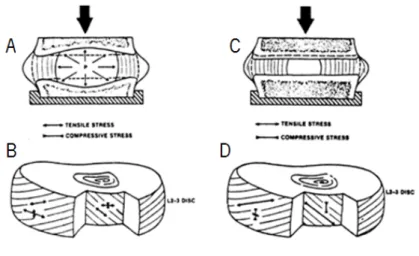
In a normal lumbar disc, the nucleus carries the compressive loadings and the annulus the tensile stresses. When the disc is degenerated this loading capacity diminishes. It happens because the amount of water retained inside the disc diminishes, and thus the tensile stresses in the collagen fibres (annulus fibrosus) become compressive loads because they are not any more activated by the nucleus [Jensen, 1980]. Figure 2.6 represents schematically the behaviours of the normal and degenerated disc under a compression loading.

Figure 2.6 – Compression loading (A) a normal non-degenerated and (C) degenerated disc. Outer annulus layers have a large tension stress along the fibres and also in the tangential peripheral direction. The inner annulus fibres have stresses of smaller magnitude (B). Annulus fibres show outer layers are subjected to increased amount

(34)

The nucleus herniation leads to a loss in the mechanical loading capacity, a decrease in the disc height and to the disc degeneration. The loss of the hydraulic and elastic properties in the disc depends on the decrease of the water’s content and therefore in a lessening of the preload effect of the nucleus; a decrease in the elastic collagen tissue in the annulus with replacement of large fibrous inelastic bands and cartilage degeneration in the end-plates [Jensen, 1980].

The disc degeneration can be identified in five different grades, and the usage of some imaging techniques analysis can help the clinical diagnosis. Non-invasive medical techniques, such as radiography, computed tomography (CT) and magnetic resonance imaging (MRI), are commonly used in medicine for the diagnosis of DDD [Wills et al., 2007].

Studies with animal discs, for example ovine discs [Reid et al., 2002], are essential due to

the difficulties in obtaining and working with human specimens. Although Smit, [2002] had shown that a quadruped can be a representative animal model for Human spine, in vitro tests have shown

that the mechanical properties of the disc cannot be restored, especially if the physiological limits of the tissues are exceeded, during the tests. Consequently, with this difficulty to correlate the disc responses to in vivo and in vitro loadings, there is a necessity to create models that allow to

virtually studying such mechanisms. The FE analysis is an important tool for simulation and to understand the stress distributions inside the disc. Knowing the different behaviours of the disc (native and degenerated) could help improve some strategies to understand the degenerative disc diseases. Obviously both the accuracy of geometrical modelling and mechanical behaviour characterization play a paramount role to ensure the reliability and significance of numerical analysis when compared with in vivo studies.

(35)

Chapter 3. Medical Image Techniques

3.1. Introduction

Nowadays, the diagnosis based on medical imaging provides an effective way to non-invasively represent the anatomy of the Human body. Several imaging techniques are available to help in the diagnosis of DDD, therapy and research of the back pain [Wills et al., 2007]. Depending on the

patient’s problem, different techniques can be used to evaluate DDD.

This chapter summarizes most common patient in vivo non-invasive data acquisition

techniques of the Human lumbar spine. Plain radiography can show bones of lumbar spine, CT depicts images of the vertebrae and, to a certain extent, images of the muscles, vessels and nerves, while MRI can provide images of the shape and internal structure of bones, disc, joints, muscles, vessels and nerves [Wills et al., 2007]. These techniques offer the possibility to produce a

set of transverse slice 2D images. Consequently these images can be used to reconstruct the 3D model after applying several imaging processing procedures and numerical methods such as denoising, smoothing, segmentation and, finally, 3D reconstruction and sampling.

3.1.1. Plain radiography

Generally, the plain radiographs are the first diagnosis technique used to obtain information about the back pain. Essentially, this technique allows examining bones structure. Disc space narrowing, development of endplate sclerosis and osteophytes and, occasionally, gas formation in the disc can be seen through radiography (Figure 3.1). Despite all of this, radiographs are not able to identify any damage in soft tissues (e.g., in the case of disc herniation) [Wills et al., 2007].

(36)

Figure 3.1 – Plain radiographs showing the following: (A) Narrowing of the L5-S1 disc space with mild osteophyte formation demonstrating mild DDD at this single level. (B) Disc space narrowing, endplate sclerosis, and osteophytes at L1-L2, L2-L3, L4-L5, and L5-S1 in this patient with marked multi-level DDD. Retrolisthesis of L3 on

L4 is also seen [Wills et al., 2007].

X-ray system consists of a vacuum tube which contains a cathode that directs a stream of electrons into a vacuum, and an anode, which collects the electrons thus forming a beam of electrons. X-ray photons are produced by this electron beam and are accelerated at high speed towards patient [Suetens, 2009].

2D representation image is obtained as the result of this interaction between the X-ray photons and the patient. Interaction between X-ray and the patient depends on the density and composition of the different body areas. The image contrast is the intensity difference in adjacent regions of the image and it depends on the attenuation coefficients, the spectrum beam, and on the thicknesses of the different tissue layers. Another important factor that influences the contrast is the absorption efficiency of the detector, which is the fraction of the total radiation hitting the detector that is actually absorbed by it. Higher absorption efficiency yields a higher contrast [Butler

(37)

3.1.2. X-ray computed tomography

The first computed tomography (CT) scanner was presented by Godfrey Hounsfield [Hounsfield, 1973]. Since then, new and improved scanners have been developed. CT has the advantage to provide a quick and non-invasive method of assessing patients. This procedure is particularly suited to high X-ray contrast structures, such as bones, and is limited in the analysis of soft-tissues like intervertebral discs and ligaments. As opposed to plain radiographies, computed tomography images allow to diagnose problems and to reveal marginal osteophytes, foraminal stenosis, disc space (vacuum phenomenon) arising and endplate sclerosis [Wills et al., 2007].

Figure 3.3 – CT scan showing complete loss of the L5-S1 disc space with severe endplate sclerosis and development of osteophytes. [Wills et al., 2007].

The CT system is simple and uses X-rays as the radiography technique. In conventional CT, the X-ray tube and the detector rotate around the stationary table3. A source that emits an X-ray beam with very high energy can be rotated around one axis while the patient is translated parallel to that axis. This beam is attenuated by absorption and scatters as it passes through the patient body with the detector measuring transmission. A computer reconstructs the image for this single slice. The patient and the table are then moved to the next slice position and the next image is obtained. This way, X-ray images of each section are digitally recorded from many angles [Butler et al., 2007; Suetens, 2009].

3 This table is where the patient is lying.

(38)

There are different generations of CT technique and Figure 3.4 shows these five types of CT scanners. In the first-generation CT scanner, the X-ray source and the detector have two motions: linear translation and rotation. The X-ray beam is narrow and the scanning time to obtain parallel-beam projections are approximately 25 minutes. The second-generation CT used narrow fan-beam geometry with 12 detectors. This scanner has two motions as first-generation: linear translation and rotation but the scanning time is too short (about 1 minute). The third-generation CT uses a fan-beam geometry but with 1000 detectors. The difference in this scanner is that no linear translation motion is necessary. The scanning time is approximately 0.5 seconds and this CT scanner is frequently used in medical imaging. The fourth-generation CT has a stationary ring detector and the X-ray source rotates around the patient. This scanning method is very fast but it is subjected of a high scattering level and it is impossible to collimate the X-rays on the detector [Zeng, 2010].Nowadays, modern CT scanners perform a helical scanning. The X-ray source and the detectors rotate while the table has linear translation in the axial direction. This type of scanner has a 2D multi-row detector and it acquires cone beam data.

Figure 3.4 – Principle of different generations of CT scanner. First (A), Second (B), Third (C), Fourth (D) and modern (E) generation scanner (adapted from [Zeng, 2010]).

(39)

The principle of this technique is based on a monochromatic X-ray beam which crosses the body and it can be absorbed. This phenomenon is described by Beer's Law:

= (3.1)

where I0 and I are the initial and final X-ray intensity, µ is the material's linear attenuation coefficient

(units 1/length) and x is the length of the X-ray path [Suetens, 2009].

Figure 3.5 – The principle of attenuation.

Similarly to the case of radiography, the attenuation of the X-ray beam is directly proportional to tissues density. This attenuation can be “measured” by the level of grey attributed to each pixel of a given image. The level of grey of each pixel is usually expressed by CT numbers in Hounsfield scale, defined as

= −

− × 1000 (3.2)

where µ (water) = 0 HU and µ (air) = -1000 HU [Butler et al., 2007; Suetens, 2009].

These values can be used to differentiate tissues in agreement with their attenuation, on a scale from +3071 (higher attenuation) to -1024 (lower attenuation) on Hounsfield scale, i.e., on 4096 levels of attenuation. The contrast resolution of CT images depends on the differences between Hounsfield values of neighbouring tissues, the larger the better. For example, bone and calcified structures have values of 200–900 HU. Some clinical applications look at air–tissue or tissue–bone contrasts on the order of 1000 HU, but other clinical exams focus on smaller soft tissue contrasts of a few HU. An optimal perception requires a suitable grey level transformation. Although better than plain X-ray in differentiating soft tissue types, CT is not as good as magnetic resonance imaging (MRI).

(40)

CT is mainly suited for bones. One of the most important advantages of this technique is the ability to reproduce a 3D structure and to represent a 2D cross-section with high accuracy. In CT, this process depends on some technological characteristics that affect image quality, such as spatial resolution, contrast resolution, linearity, noise and artefacts.

3.1.2.1. Micro-computed tomography

Micro-computed tomography (or micro-CT) is a new and innovative field of non-invasive imaging technique. The main advantage of this scanning technique is its micro scale. Recently, several studies [Holdsworth et al., 2002; Ritman, 2004] have been carried out with small animals using

this technique to obtain high-resolution 3D models with application on, for instance, monitoring efficacies of drugs in disease treatment, among others.

Micro-CT is based on the same principle of conventional CT, but with a much higher resolution than the one in conventional clinical scanners. Clinical tomography scanners have resolutions around one millimetre, while micro-CT scanners may have resolutions below five microns [Ritman, 2004].

3.1.3. Magnetic Resonance Image

Magnetic resonance imaging (MRI) is another medical imaging technique frequently used both in medical diagnosis and as surgery supporting tool, with the ability to produce high quality images. Usually, MRI provides detailed information about changes associated with DDD. In case of soft tissues, the contrast is better than within CT, what shall allow an easier and more effective identification of the most relevant tissue’s domains, for instance inside an intervertebral disc. MRI also allows a better visualization of the vertebral marrow, the ligaments and contents of the spinal canal [Fujiwara et al., 1999]. In cases such as infections or tumours, the MRI provides information

about the source of the pain. However, in cases where the pain is due to mechanical causes (most common cases) the MRI does not provide any additional information.

MRI is a medical imaging technique based on a magnetic field (B0) and pulses of radio waves to produce images of internal organs and structures. MRI uses non-ionizing radio frequency (RF) signals to acquire its images and it is best suited for non-calcified tissues. MRI depends on protons mobility in tissues, and since most protons in biological tissues are in water, normal clinical applications involve the imaging of hydrogen nuclei (protons). One can assume that the

(41)

protons in the patient tissues behave like tiny bar magnets, which are normally randomly oriented in space. When the patient is placed within a strong magnetic field, some of the atomic nuclei are aligned with respect to such external magnetic field (Figure 3.6). The protons behave like miniature magnets and spin at a specific frequency. When the protons are back to their equilibrium position (i.e., relax to a lower energy state), they release energy like a small radio transmitter. These radio signals are detectable (by an aerial) and electronically amplified, in order to create a magnetic resonance image. Human spine MRI exams, used to identify back disorders, IVD diseases and spinal cord disorders, are usually performed using clinical magnetic fields (1.5 and 3 Tesla), with specific phased-array coils for spinal MRI exams.

Figure 3.6 – The tiny bar magnets (A) before and (B) after the tissues being placed within a strong magnetic field.

When the proton relaxes, there are two processes before it emits radio waves: the longitudinal recovery (which has a recovery time, T1) and the transverse relaxation (with a relaxation time, T2). The relative proportions of T1 and T2 varies for different tissues. In MRI studies of IVD degeneration, the qualitative analysis of T1-weighted and T2-weighted images in the sagittal and axial planes are used. As showed in Figure 3.7, these processes may highlight the disc degeneration through the modification of the signal intensity.

Figure 3.7 – T1-weighted (A) and T2-weighted (B) sagittal MRI demonstrating a disc herniation at L4-L5 [Wills et al., 2007].

(42)

Generally, the T1-weighted imaging is used to study the abnormalities of the spine. However, lower signal intensity (T2-weighted) images are associated with degenerative IVDs and a loss of water content of the disc. By measuring the disc height, the signal intensity alteration and the signal-to-noise ratio it is possible to complete these exams [Wills et al., 2007].

3.1.3.1. Micro Magnetic Resonance Imaging

Nowadays, with the recent advances in medical imaging techniques, it is possible to obtain MRI images with higher resolution via micro-MRI scanners [Majumdar et al., 1997]. This technique

allows to distinguish different types of tissues with higher detail due to its micro-scale (μm) resolution. Nevertheless, the low signal-to-noise ratio and the inhomogeneous signal becomes an obstacle during model reconstruction from micro-MRI images [Strolka et al., 2003].

Recently, several studies with micro-MRI techniques have been developed. Among others, Uffen and co-workers evaluated the detection capacity of different tissues with micro-MRI in nine animals that were part of a goat spinal fusion study [Uffen et al., 2008]. Liu and co-workers

demonstrated the importance of micro-MRI technique for in vivo trabecular bone morphometry [Liu et al., 2010]. Bonny and co-workers demonstrated that the high-quality can be achieved at 9.4 T

using micro-MRI images of an in vivo mouse spinal cord. The increasing availability of clinical high

resolution MRI scanners will support the spread on many clinical application of this technology in a near future [Bonny et al., 2004]. The micro-MRI technique is a valuable tool to aid in future clinical

evaluations and decisions.

3.1.4. Other medical image techniques

Ultrasound, discography and CT-myelography, are also commonly used in clinical diagnosis of the low back pain. However, these techniques present some restrictions - for example, the use of contrast agents that are invasive and do not provide good exam conditions for the patient or their low image resolution, which does not allow to clearly distinguish the different anatomical regions of interest in the images.

3.2. Comparison of medical image resolution

The resolution of a medical image depends on the imaging method, the characteristics of the equipment, and the imaging values selected by the operator. These values will influence the image

(43)

synthesis of the different and most typical resolutions of the medical imaging techniques addressed in this chapter, as well as their main characteristics and applications.

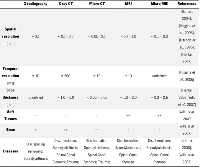
Table 3.1 – Resolution and some characteristics of images from different medical imaging techniques.

X-radiography X-ray CT Micro-CT MRI Micro-MRI References

Spatial resolution [mm] ≈ 0.1 ≈ 0.1 - 0.5 ≈ 0.05 - 0.1 ≈ 0.7 - 1.0 ≈ 0.1 – 0.3 [Ritman, 2004]; [Higgins et al., 2006]; [Hitchon et al., 1995]; [Henke, 2007] Temporal resolution [ms] ≈ 10 ≈ 500 ≈ 10 ≈ 10 undefined [Higgins et al., 2006] Slice thickness [mm] undefined ≈ 1.0 – 5.0 ≈ 0.05 – 0.06 ≈ 1.0 – 3.0 ≈ 0.3 – 0.6 [Henke, 2007; Wills et al., 2007] Soft Tissues − − − − ++ ++ [Wills et al., 2007

Bone + ++ ++ − − [Wills et al.,

2007] Diseases Disc spacing narrowing; Spondylarthrosis Disc herniation; Spondylolisthesis; Spinal Canal Stenosis; Trauma; Disc herniation; Spondylolisthesis; Spinal Canal Stenosis; Trauma; Disc herniation; Spondylolisthesis; Spinal Canal Stenosis Disc herniation; Spondylolisthesis; Spinal Canal Stenosis [Krämer, 2008]; [Wills et al., 2007]

(44)

(45)

Chapter 4. Three-dimensional reconstruction from

medical imaging

The starting point for the 3D geometrical modelling by finite elements of a motion segment is the generation of a 3D voxel-based geometrical model, obtained after denoising, smoothing and segmentation of a set of 2D medical images. This chapter addresses and describes the procedures for 3D reconstruction from 2D medical imaging obtained from computed tomography (CT), micro-CT, magnetic resonance imaging (MRI) or micro-MRI, 3D reconstruction techniques and some segmentation algorithms. Advantages and drawbacks of the main reconstruction algorithms and procedures are illustrated with the 3D reconstruction of a goat IVD from real medical imaging data obtained from MRI and micro-MRI using the image processing software ScanIP (Simpleware Ltd, Exeter, UK).

4.1. Introduction

Medical imaging techniques (detailed in Chapter 3) enable one to create a set of related 2D images, where each 2D image represents a thin "slice" of the body. This set of 2D images one shall be able to reconstruct a 3D voxel-based model. Nevertheless, the 3D model reconstruction process is not linear and the images shall be, in most of cases, subjected to image processing. The fundamentals of image processing are based on parameters that are inherent to images, such as image resolution. The image resolution is the level of detail of an image and a measurement of its quality, i.e., resolution defines pixel size. Higher resolution means more image detail, which is affected by interrelated factors (e.g., matrix size, pixel size, field-of-view, voxel size, slice thickness, focal spot size and blur) [Suetens, 2009].

In an imaging acquisition, a so-called matrix is used to break the image into columns and rows of tiny squares. Each elemental unit, called pixel, is known to be the smallest component of an image. Thus, a given amount of pixels gives rise to an image. The matrix size refers to how many pixels are used in the definition of the grid. For example, a 512 matrix will have 512 pixels

(46)

across the rows and 512 pixels down the columns. The most common matrix sizes used in medical images are 256, 512 and 1024. Another image parameter is the field-of-view (FOV) which represents the maximum size occupied by the object in the matrix. One of the most common problems that an image may present is a high FOV, which may cause a blur image and low resolution images [Suetens, 2009].

During the 3D reconstruction procedure from 2D images, each pixel is converted into a voxel (3D unit that represent a 2D pixel unit), giving a kind of depth to the image, as shown in Figure 4.1. A voxel represents a volume of patient's data. The length of the voxel correlates to the operator selection of slice thickness. Therefore, the slice thickness plays an even larger role in volume averaging (as well as the subsequent spatial resolution or slice spacing) than either display FOV or matrix size.

Figure 4.1– The pixel and the voxel representation.

Generally, a voxel has a parallelepiped shape, which can be reduced to a cube in special cases. Each voxel has a defined volume and a level of grey resultant from medical imaging acquisition process. Thus, this level of grey is the paramount property attributed to each voxel, given its physical meaning. This grey scale is defined by a large spectrum of representations of shades (216) between white and black. The grey scale created especially for tomographic images has a unit of measure called Hounsfield (see section 3.1.2 - X-ray computed tomography).The tomographic image consists in more than 2000 tonalities, but the human eye is only able to distinguish between 10 to 60 grey tonalities. Because of this, and to make the differentiation between structures easier, computational resources (such as feature called window) enable to

narrow the values of the grey scale. This works as an alteration in the grey tones of the image accordingly to the human vision of the tomography data. However, it is not possible to use at the same time different sets of window (i.e., bone, fat, soft tissue) [Suetens, 2009].