Low complexity detection for SC-FDE massive MIMO systems

(1)

Setembro, 2016

David Oliveira Borges

Licenciado em Ciências da Engenharia Electrotécnica e de Computadores

Low complexity detection for

SC-FDE massive MIMO systems

Dissertação para obtenção do Grau de Mestre em Engenharia Electrotécnica e de Computadores

Orientador: Prof. Dr. Rui Dinis, Professor Associado com Agregação, Faculdade de Ciências e Tecnologia - UNL

Co-orientador: Prof. Dr. Paulo Montezuma, Professor Auxiliar, Faculdade de Ciências e Tecnologia - UNL

Júri:

Presidente: Prof. Dr. Luís Oliveira – FCT/UNL

Vogais: Prof. Dr. Luís Bernardo – FCT/UNL (Arguent e)

(2)

(3)

Low complexity detection for SC-FDE massive MIMO systems

(4)

(5)

(6)

(7)

vii

Agradecimentos

Aos professores e orientadores desta tese Rui Dinis e Paulo Montezuma por toda a paciência e disponibilidade que demonstraram no decorrer desta tese. Por todo o conhecimento, motivação e boa disposição, obrigado.

À minha família, agradeço pela confiança e motivação para nunca desistir, por tudo o que fizeram por mim a nível pessoal e académico, estiveram sempre ao meu lado para me dar força nos bons e maus momentos.

A todos os amigos que, mais de perto ou não tanto, estiveram presentes no decorrer deste percurso académico, que tantos bons momentos nos proporcio-nou, beijinhos e abraços.

(8)

(9)

ix

Abstract

Nowadays we continue to observe a big and fast growth of wireless com-munication usage due to the increasing number of access points, and fields of application of this technology. Furthermore, these new usages can require higher speed and better quality of service in order to create market. As example we can have: live 4K video transmission, M2M (Machine to Machine communication), IoT (Internet of Things), Tactile Internet, between many others.

As a consequence of all these factors, the spectrum is getting overloaded with communications, increasing the interference and affecting the system's per-formance. Therefore a different path of ideas has been followed and the commu-nication process has been taken to the next level in 5G by the usage of big arrays of antennas and multi-stream communication (MIMO systems) which in a greater scale are called massive MIMO schemes. These systems can be combined with an SC-FDE (Single-Carrier Frequency Domain Equalization) scheme to im-prove the power efficiency due to the low envelope fluctuations.

(10)

x

With this approach we want to minimize the ICI (Inter Carrier Interference) in order to have almost independent data streams and to produce a low complexity code, so that the receiver's performance doesn't affect the total system's perfor-mance, with a final objective of increasing the data throughput in a great scale.

(11)

xi

Resumo

Hoje em dia continuamos a assistir a um grande e rápido crescimento da utilização da comunicação sem fios, devido ao aumento do número de pontos de acesso e campos de aplicação desta tecnologia. Além do aumento na transferên-cia de dados, os novos tipos de utilização podem exigir uma maior velocidade e melhor qualidade de serviço, seja por necessidade dos utilizadores ou por neces-sidade de mercado. Como exemplo, podemos ter: transmissão em direto de vídeo 4K, M2M (comunicação máquina a máquina), IoT (Internet das coisas), Internet Táctil, entre muitas outras.

Como consequência do aumento do número de utilizadores, o espectro está a ficar sobrecarregado com comunicações, aumentando a interferência. Desta forma, um caminho diferente de ideias tem sido seguido e o processo de comu-nicação foi levado para um próximo nível no 5G, com o uso de grandes conjuntos de antenas e vários fluxos de dados (sistemas MIMO), que em maior escala são chamados de MIMO massivo.

(12)

xii

Ratio Detector), IB-DFE (Iterative Block Decision Feedback Equalizer) e uma pro-posta de recetor combinando MRD (ou EGD) e IB-DFE. Com esta abordagem queremos minimizar a interferência, de modo a obtermos fluxos de dados quase independentes, e produzir um código de baixa complexidade para que o desem-penho do recetor não afete o desemdesem-penho total do sistema, com um objetivo final de aumentar a taxa de transferência de dados.

Palavras-chave: 5G, MIMO massivo, Mono-portadora, Igualização no Domínio

(13)

xiii

ACRONYMS

3G 3rd Generation

3GPP 3rd Generation Partnership Project

4G 4th Generation

5G 5th Generation

BER Bit Error Rate

BS Base Station

CSI Channel State Information

DFE Decision feedback equalization

DFT Discrete Fourier Transform

DPC Dirty Paper Coding

EGD Equal Gain Detector

FD Frequency Domain

FDE Frequency Domain Equalization

FDM Frequency Division Multiplexing

FFT Fast Fourier Transform

HSPA High Speed Packet Access

IB-DFE Iterative Block Decision Feedback Equalization

(14)

xiv ICI Inter-Carrier Interference

IFDE Iterative Frequency Domain Equalization

IFFT Inverse Fast Fourier Transform

ISI Inter symbol Interference

LOS Line of sight

LTE Long Term Evolution

MIMO Multiple Input Multiple Output

MMSE Minimum Mean Square Error

MRD Maximum Ratio Detector

MRT Maximum Ratio Transmission

MU-MIMO Multiple User-Multiple Input Multiple Output

OFDM Orthogonal Frequency-Division Multiplexing

OFDMA Orthogonal Frequency-Division Multiple Access

PAPR Peak Average Power Ratio

QoE Quality of Experience

QoS Quality of Service

QPSK Quadrature Phase Shift Keying

RSSI Received signal strength indication

SC Single Carrier

SC-FDE Single-Carrier Frequency Domain Equalization

SNR Signal-to-Noise Ratio

SU-MIMO Single User-Multiple Input Multiple Output

TD Time Domain

TDMA Time Division Multiple Access

UE User Equipment

(15)

xv

3.2.1 Switching_______________________________________________ 25 3.2.2 Selection _______________________________________________ 26 3.2.3 Zero Forcing ____________________________________________ 27 3.2.4 Equal Gain Combining ____________________________________ 29 3.2.5 Maximum Ratio Combining ________________________________ 30 3.3 MINIMUM MEAN SQUARED ERROR _________________________________________ 31

(16)

xvi

3.4.1 IB-DFE with Soft Decisions ________________________________ 35 3.5 SINGULAR VALUE DECOMPOSITION (SVD) __________________________________ 37

4 ITERATIVE MASSIVE MIMO RECEIVERS _______________________________________ 39

4.1 EGD/MRD+IB-DFE ________________________________________________________ 40

4.2 PERFORMANCE RESULTS _____________________________________________________ 42

4.2.1 Iterations effect __________________________________________ 42

4.2.1.1 Results of iterations effect on EGD _______________________________________ 43

4.2.1.2 Results of iterations effect on MRD_______________________________________ 44

4.2.1.3 Results of iterations effect on IB-DFE _____________________________________ 45 4.2.2 Increasing number of antennas _____________________________ 46

4.2.2.1 Increasing ratio_________________________________________________________ 46

4.2.2.2 Constant ratio __________________________________________________________ 47

4.2.2.3 Increasing transmitt ing antennas _________________________________________ 49

5 CONCLUSIONS___________________________________________________________________ 51

5.1 FINAL CONSIDERATIONS ____________________________________________________ 51

5.2 FUTURE WORK ______________________________________________________________ 52

ATTACHMENTS ___________________________________________________________________ 53

(17)

xvii

List of figures

FIG.1.1–MULTIPATH PROPAGATION AND TIME DISPERSION EFFECT [4]………....…2

FIG.2.1–4G VS 5G ANTENNA (ACTIVE PHASED-ARRAY ANTENNA).………6

FIG.2.2–PHOTO OF THE ANTENNA ARRAY OF THE LUMAMI TESTBED AT LUND UNIVERSITY IN SWEDEN…….……….7

FIG.2.3-POSSIBLE LANDSCAPE AND PERFORMANCE AIMS [12].……….….……….8

FIG.2.4–MIMO2X2 CHANNEL CONFIGURATION.……….……….…….10

FIG.2.5-MASSIVE MIMO SCENARIO.……….……….………11

FIG.2.6- ANTENNA CONFIGURATIONS AND DEPLOYMENT SCENARIOS FOR A MASSIVE MIMO BASE STATION………….12

FIG.2.7–SC-FDERECEIVER STRUCTURE [17] ADAPTED.1……….…….………..14

FIG.2.8-OFDM VS SC-FDE[20] ADAPTED.……….………15

FIG 2.9–TYPICAL TRANSMISSION VS BEAMFORMING WAVES.……….……….…18

(18)

(19)

1

1 Introduction

1.1 Motivation and Scope

Wireless communications have experienced exponential growth in the last few decades due to the development of reliable solid-state radio frequency hard-ware in the 1970s. Since then, innumerous standards have been developed for wireless systems throughout the world [1].

The increasing need for fast and reliable wireless communication links has led to some new path of ideas and systems with multiple antennas located at both the transmitter and the receiver side is one of them. Input Multiple-Output (MIMO) systems are able to increase very significantly the capacity and hence achieve higher transmission rates than the one-sided array links.

The notorious Shannon theorem for capacity of bandlimited Gaussian channels shows that there is a fundamental limit (channel capacity) for transmis-sion data rate over these channels [2]. With the advances in communication the-ory and the growth of sophisticated signal processing and computation tech-niques, the possibility of achieving the fundamental information limit on the channel capacity seems higher than ever before.

The next generation of wireless systems is expected to provide end-to-end communication where voice, data and streamed multimedia can be served to

us-ers at “anytime, anywhere” basis with an aim of Gbits/s. Data throughput has long been one of the most important performance indicators for communication systems.

(20)

2

sion Multiplexing) and SC (Single Carrier) modulation combined with FDE (Fre-quency Domain Equalization). This thesis will focus on the SC-FDE technique which is more suitable for uplink due to its lower PAPR (Peak to Average Power Ratio) [3].

As a direct consequence of the increase in data rates, the effects of multi-path propagation, inter-symbol interference (ISI) have been augmented, result-ing in the need for more complex equalizers. The complexity of the equalization process is enlarged even more in MIMO systems due to the addition of extra transmit and receive antennas.

Fig. 1.1–Multipath propagation and time dispersion effect [4].

(21)

3

feedback part of the DFE (Decision Feedback Equalization) to the transmitter side to avoid the error propagation problem.

All this increased complexity in the analog and digital domain has its dis-advantages. This thesis will focus on the receiver design, having in mind the high computational processing needed for massive MIMO schemes. The delay that can be introduced by these complex scenarios is going against the 5G ideology which aims an ultra-low latency. For this reason the complexity of the receivers used in massive MIMO schemes should be as low as possible without compro-mising the desired QoS.

1.2 Objectives

The objective of this thesis is, based on state of the art technology, to de-velop and test a low complexity detector for SC-FDE massive MIMO systems. This objective includes the development, test and usage of a massive MIMO sys-tem simulator, implementing the scenario described in the next section, in which both proposed receivers were tested. All these tasks were accomplished using a numerical computing environment, MATLAB®.

A low-complexity iterative frequency-domain receiver combined with the MRD (Maximum Ratio Detector) and other based on EGD (Equal Gain Detector) are proposed. These receivers do not require matrix inversions and have excel-lent performance, being able to approach the MFB (Matched Filter Bound) after just a few iterations, even for a moderate number of antennas.

The receivers were tested and studied by analyzing the impact of the number of used antennas in each sender and receiver at a time. By varying the number of antennas in transmitter and receiver separately, changing the ratio between receiving and transmitting antennas (R:T) and ultimately increasing the number at both ends at the same time, different scenario types were analyzed and compared. The BER (Bit Error Rate) values, as well as the performance of

(22)

4

1.3 Organization

This thesis is divided in five sections as described bellow:

Chapter 2 contains an introduction and a literature review about related work and used technologies. An overview about 5G is presented, followed by a description of millimeter wave systems that includes MIMO and massive MIMO. It continues with the explanation of SC-FDE, precoding and its particular usage, beamforming. Chapter ends with the proposed scenario characterization.

In Chapter 3 overall discrete model is presented, basic detections schemes are explained and the receiver’s algorithms are introduced.

Chapter 4 contains an overview on iterative massive MIMO receivers and the description of the receivers’ proposed model and algorithms. After this, per-formance results and conclusions are presented.

Finally, Chapter 5 contains the overall conclusions and possible future work that can be done by taking this dissertation as reference.

A paper with the performance analysis of these receivers was produced in the elaboration of this thesis and its presented as an attachment.

1.4 Contributions

During the development of this thesis, after implementing and testing the proposed receivers in simulations, some observed results were considered moti-vating. In order to validate this interest with the community, a scientific paper a scientific paper was produced and summited to a conference. As this interest was shared among the evaluators, the paper was accepted in the 2016 IEEE Global Conference on Signal and Information Processing which had place from 7th_{to 9}th_of

(23)

5

2 MIMO techniques for SC modulation

2.1 General 5G

Massive MIMO schemes (Multiple-Input, Multiple-Output) involving several tens or even hundreds of antenna elements are expected to be central technologies for 5G systems. The integration of millimeter-wave (mmWave) and MIMO can achieve orders of magnitude increase in rates due to larger bandwidth and greater spectral efficiency [6]. This makes mmWave MIMO as a promising technique for future 5G wireless communication systems. Extremely higher data rates, large BW (Bandwidth) and ultra-low latencies required by 5G wireless can-not be achieved by the simple evolution of current wireless technologies [7].

This chapter characterizes some of the disrupting technologies that will be useful in enabling the 5G transition. Starting by a review of the state of the art, mm-wave systems, MIMO and massive MIMO are explained. Their advantages and obstacles are presented, as well as suitable techniques like SC-FDE and Pre-coding. It finished with the description of the proposed and simulated general scenario, regarding a massive MIMO communication system.

2.2 An Extension to Higher Frequency/Millimeter Waves

(24)

6

new spectrum for mobile telecommunications below 6 GHz are not very favora-ble for transition to 5G architectures.

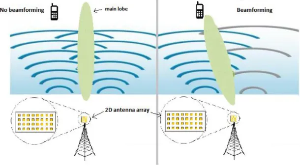
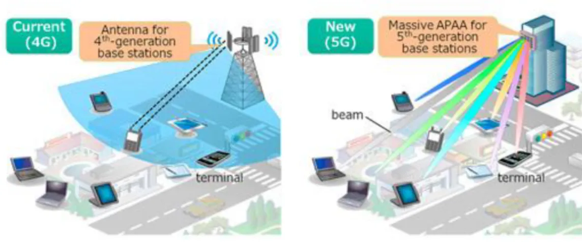
4G vs 5G antenna technology

Fig. 2.1–4G vs 5G antenna (Active Phased-Array Antenna).

Recent advances in mobile communication systems and devices operating at higher microwave and mm-wave frequencies, combined with improvements in antenna and RF component technologies, have opened the doors to using non-conventional bands for cellular applications. Such advancements will help enable dense small cell deployments over a diverse set of higher spectrum bandwidth. Such deployments will be an important 5G’s usage scenario as there will be con-tinued need to meet exponential growth in traffic demand and to address the requirement for gigabit data rates everywhere, including at cell edge, as exem-plified in Fig. 2.1. It is expected that to meet 5G network requirements, operating over this higher part of spectrum (e.g. 10-100+ GHz) will be needed to deploy indoors and/or outdoors.

With the potential use of frequencies higher than 10 GHz as well as mm-wave deployment, the available spectrum might rise from a typical 500MHz to several GHz, making many bands therein seem promising. Nevertheless, with the increase in carrier frequency, signal penetration loss increases, diffracted sig-nals become very weak and thus the importance of line-of-sight (LOS) signal as well as reflected signal component increases. Although propagation at mm-wave bands covering 30-300GHz presents some challenges, recent measurements indi-cated distance dependent LOS communication channel characteristics similar to microwave bands. Non-LOS communication remains a good option [8].

(25)

7

Millimeter wave systems can operate in noise-limited conditions rather than interference-limited situations by reducing the impact of interference with narrow beam adaptive arrays. When beams are blocked by obstacles, the use of adaptive array processing algorithms can help to adapt quickly. The smaller wavelength associated with higher frequencies of mmWave enables to pack a large antenna array in a small physical dimension, as we can observe in Fig. 2.2 [9]. The large antenna array can provide sufficient antenna gain to compensate for the severe attenuation of mmWave signals due to path loss, oxygen absorp-tion, and rainfall effect [10]. Additionally, the large antenna array can also sup-port the transmission of multiple data streams to improve the spectral efficiency through the use of precoding [11].

Antenna array at Lund University in Sweden

Fig. 2.2 –Photo of the antenna array of the LuMaMi testbed at Lund University in Sweden.

The array consists of 160 dual-polarized patch antennas. It is designed for a carrier fre-quency of 3.7 GHz and the element-spacing is 4 cm (half a wavelength).

(26)

8

Emerging wide area wireless services and usage cases are shaping the 5G vision and driving the 5G technology requirements. Ultra-high throughput, hancement in network capacity, ultra-low latency, ubiquitous connectivity, en-ergy efficiency, high reliability, low-cost devices and QoE are just some of the requirements that the next generation wireless needs to achieve. The race is cur-rently on to find the wireless communication network, system architectures, and technologies that will bring the big data to the world beyond 2020.

5G possible landscape and aimed performance

Fig. 2.3 - Possible landscape and performance aims [12].

2.3 MIMO

(27)

9

802.11ac (Wi-Fi), HSPA+ (3G), WiMAX (4G), and Long Term Evolution (4G LTE). More recently, MIMO has been applied to power-line communication for 3-wire installations as part of ITU G.hn standard and HomePlug AV2 specifica-tion.

At one time in wireless the term “MIMO” referred the mainly theoretical use of multiple antennas at both the transmitter and the receiver. In modern

us-age, “MIMO” specifically refers to a practical technique to send and receive sev-eral data signals on the same radio channel, at the same time, via multipath prop-agation. In Fig. 2.4 we can observe what it would be a channel configuration of 2 transmitting and 2 receiving antennas in a MIMO scheme. MIMO is fundamen-tally different from smart antenna techniques developed to enhance the perfor-mance of a single data signal, such as beamforming and diversity [13]. MIMO applied in cellular systems brings four improvements:

• increased data rate: due to the usage of more antennas, the more inde-pendent data streams can be transmitted and the more terminals can be served simultaneously;

• enhanced reliability: increasing number of transmitting antennas cre-ates more distinct paths for the radio signal to propagate over;

• improved energy efficiency: the base station can focus its emitted en-ergy into the spatial directions where it knows that the terminals are located;

• reduced interference: the base station can purposely avoid transmitting into directions where spreading interference would be harmful.

Other benefits of massive MIMO include the extensive use of inexpensive low-power components, reduced latency, simplification of the media access control (MAC) layer, and robustness to intentional jamming. All improvements cannot be achieved simultaneously, and there are requirements on the propagation con-ditions, but the mentioned bullets are the general benefits.

(28)

10

General 2x2 MIMO channel configuration

Fig. 2.4 –MIMO 2x2 channel configuration.

The drawbacks of MIMO is the higher complexity of the analog and digital do-mains. For point-to-point links, complexity at the receiver is usually a greater concern than transmitter’s one. For example, the complexity of optimal signal detection alone grows exponentially with the number of transmitting antennas. In multiuser systems, complexity at the transmitter is also a concern since ad-vanced coding schemes must often be used to transmit information simultane-ously to more than one user while maintaining a low level of inter-user interfer-ence. This prohibitive complexity motivates a continuous search for computa-tionally efficient, considering optimal or suboptimal detectors.

2.4 Massive MIMO

Massive MIMO is an emerging technology that scales up MIMO by several orders of magnitude compared to current state-of-the-art. With massive MIMO, we think of systems that use antenna arrays with a few hundred antennas, sim-ultaneously serving many tens of mobile terminals at the same time-frequency resource. For example, a base station (BS) equipped with an array of M active antenna elements, using these to communicate with K single-antenna (or not) terminals.

(29)

11

future broadband (fixed and mobile) networks which will be energy-efficient, se-cure, and robust, and will use the spectrum efficiently.

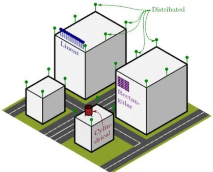
Many different configurations and deployment scenarios for the antenna arrays used by a massive MIMO system can be envisioned, as we can see at the example in Fig. 2.6. Each antenna unit would be small, and active, preferably fed via an optical or electric digital bus.

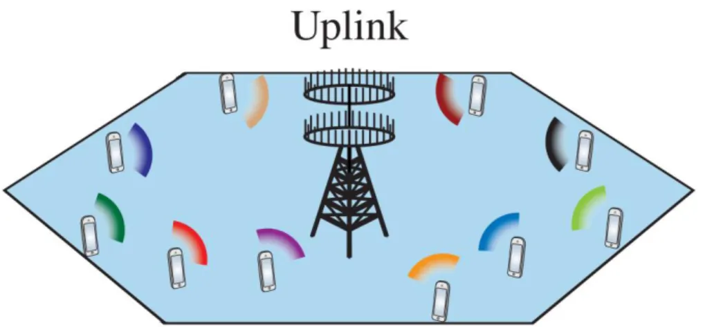
Massive MIMO scenario using beamforming

Fig. 2.5 - Massive MIMO scenario.

Massive MIMO relies on spatial multiplexing that depends on the base

station’s channel knowledge accuracy, both on the uplink and the downlink. On the uplink, this task can be easy to accomplish by having the terminals sending pilots. Then, combining these pilots and additional information that can be taken from data, base station estimates the channel responses to each of the terminals. The downlink case turns out to be more difficult. In conventional MIMO systems, like the LTE standard, the base station sends out pilot waveforms, based on which the mobile terminals estimate the channel responses and quantize the ob-tained estimates to then feed them back to the base station. This will not be fea-sible in massive MIMO systems, at least not when operating in a high-mobility environment, for two reasons:

(30)

12

Possible massive MIMO antenna configuration

Fig. 2.6 - Possible antenna configurations and deployment scenarios for a massive MIMO base station.

 Second, the number of channel responses that each terminal must estimate is also proportional to the number of base station antennas. Hence, the uplink resources needed to inform the base station about the channel re-sponses would be up to a hundred times larger than in conventional sys-tems. Generally, the solution is to operate in TDD mode, and rely on reci-procity between the uplink and downlink channels [14].

The canonical massive MIMO system operates in TDD mode, where uplink and downlink transmissions take place in the same frequency resource but are sepa-rated in time. The physical propagation channels are reciprocal—meaning that the channel responses are the same in both directions—which can be utilized in TDD operation. In particular, massive MIMO systems exploit the reciprocity to estimate the channel responses on the uplink and then use the acquired channel state information (CSI) for both uplink receive combining and downlink transmit precoding of payload data.

(31)

13

There are several good reasons to operate in TDD mode. Firstly, only the BS needs to know the channels to process the antennas’ signals coherently. Sec-ondly, the uplink estimation overhead is proportional to the number of terminals, but independent of M. This makes the protocol fully scalable with respect to the number of service antennas. Furthermore, basic estimation theory tells us that the estimation quality (per antenna) is not reduced by adding more antennas at the BS. In fact, the estimation quality improves with M if there is a known corre-lation structure between the channel responses over the array [3].

Since fading makes the channel responses vary over time and frequency, the estimation and payload transmission must fit into a time/frequency block where the channels are approximately static. The dimensions of this block are given by the coherence bandwidth Bc Hz and the coherence time Tc s, which fit

τ =BcTc transmission symbols. Massive MIMO can be implemented either using single-carrier or multi-carrier modulation.

2.5 SC-FDE

Despite the success of OFDM, this approach suffers from well-known drawbacks such as a large PAPR (Peak-to-Average Power Ratio), intolerance to amplifier nonlinearities, and high sensitivity to carrier frequency offsets. An al-ternative low-complexity approach to mitigate ISI is the use of FDEs (Frequency Domain Equalizers) in SC (Single Carrier) communications.

Systems employing FDE are closely related to OFDM systems. In fact, in both cases digital transmission is carried out blockwise, and relies on FFT/IFFT operations. Therefore, SC systems employing FDE enjoy a similar complexity to OFDM systems with the advantages of not having the stringent requirements of highly accurate frequency synchronization and linear power amplification as in OFDM, which can leverage the usage of cheaper components in user terminals with a high efficiency. The substantial lower computational complexity of FDEs compared to their TD (Time Domain) equalization counterparts is also worth to mention.

(32)

14

(2.1)

Fig. 2.7 –SC-FDE Receiver structure [17] adapted.

The first proposal of SC-FDE (Single Carrier Frequency-Domain Equaliza-tion) in digital communication systems dates back to 1973 [18].

Block transmission techniques, with appropriate cyclic prefixes and em-ploying FDE techniques, have been shown to be suitable for high data rate trans-mission over severely time-dispersive channels [19]. Two possible alternatives based on this principle are OFDM and SC modulation using FDE (or SC-FDE). Due to the lower envelope fluctuations of the transmitted signals and, implicitly a lower PAPR (Peak-to-Average Power Ratio), SC-FDE schemes are especially interesting for the uplink transmission (i.e., the transmission from the mobile ter-minal to the base station), being considered for use in the upcoming LTE cellular system.

As we can observe in Fig. 2.8, SC-FDE is a modulation where each symbol

occupies the total band allocated for the channel, so that the symbol’s energy is

distributed along the transmission band. The complex envelope of an N-symbol block (assuming that N is even) can be written as

𝑠(𝑡) = ∑ 𝑠_𝑛𝑟(𝑡 − 𝑛𝑇_𝑠)

𝑁 2 −1

𝑛=−𝑁2

,

where 𝑟(𝑡) represents the transmitted impulse, 𝑇_𝑠 is the symbol duration in sec-onds and 𝑠_𝑛 is a complex coefficient representing the 𝑛𝑡ℎ symbol resulting from a direct mapping rule of the original data bits into a selected signal constellation

(33)

15

(2.2)

(2.3) OFDM vs SC-FDE frequency usage

Fig. 2.8- OFDM vs SC-FDE [20] adapted.

If we apply the Fourier Transformation (FT) to both sides of the previous expression we obtain the frequency-domain equivalent of the signal

𝑆(𝑓) = Ӻ{𝑠(𝑡)} = ∑ 𝑠𝑛𝑅(𝑓)𝑒𝑥𝑝(−𝑗2𝜋𝑓𝑛𝑇𝑠) 𝑁

2 −1

𝑛=−𝑁2

,

where 𝑅(𝑓) represents the FT of 𝑟(𝑡). We can easily conclude that the transmis-sion band associated to each symbol 𝑠_𝑛 is the band occupied by 𝑅(𝑓).

The SC-FDE receiver can be easily extended to an L-branch diversity sce-nario. In this case, the frequency-domain samples at the FDE’s output are given by

𝑆̃_𝑘 = ∑ 𝐹_𝑘(𝑙)𝑌_𝑘(𝑙)

𝐿

𝑙=1

,

(34)

16

(2.4)

2.6 Precoding

Precoding is a generalization of beamforming to support multi-stream (or multi-layer) transmission in multi-antenna wireless communications. In conven-tional single-stream beamforming, when the receiver has just one antenna, the same signal is transmitted by each of the transmit antennas with appropriate weighting (phase and gain) such that the signal power is maximized at the re-ceiver output. When the rere-ceiver has multiple antennas, single-stream beam-forming cannot simultaneously maximize the signal level at all of the receive an-tennas. In order to maximize the throughput in multiple receive antenna sys-tems, multi-stream transmission is generally required.

In point-to-point systems, precoding means that multiple data streams are sent by the transmit antennas with independent and appropriate weightings such that the link throughput is maximized at the receiver output. In multi-user MIMO, the data streams are intended for different users (known as SDMA) and some measure of the total throughput (e.g., the sum performance or max-min fairness) is maximized. In point-to-point systems, some of the benefits of precod-ing can be realized without requirprecod-ing channel state information at the transmit-ter, while such information is essential to handle the inter-user interference in multi-user systems.

2.6.1 Precoding technique

Precoding exploits transmit diversity by weighting the information streams, i.e. the transmitter sends the precoded information to the receiver con-sidering the pre-knowledge of the channel. The receiver is a simple detector, such as a matched filter, and does not have to know the channel side information. This technique will reduce the corrupted effect of the communication channel. For in-stance, when information 𝑺 is sent, it passes through the channel 𝑯 and Gaussian noise, 𝑵, is added. The received signal at the receiver front-end will be

𝑹 = 𝑺𝑯 + 𝑵.

(35)

17

(2.5)

(2.6)

Let’s call 𝑯_𝑒𝑠𝑡 the estimated channel, hence for a system with precoder the information will be coded as

𝑺 𝑯_𝑒𝑠𝑡 .

The received signal will be

𝑹 = ( 𝑯

𝑯_𝑒𝑠𝑡) 𝑺 + 𝑵 .

If the estimation is perfect, 𝑯_𝑒𝑠𝑡 = 𝑯 and 𝑹 = 𝑺 + 𝑵.

The name of this method is “precoding” because it’s a preprocessing tech-nique that uses transmit diversity and it is similar to equalization, however, it’s done in the transmitter side. The channel equalization performed by precoder aims to minimize channel errors, but the precoder aims to minimize the error in the receiver output.

2.6.2 Precoding for Multi-user MIMO Systems

In multi-user MIMO, a multi-antenna transmitter communicates simulta-neously with multiple receivers (each having one or multiple antennas). This is known as space-division multiple access (SDMA). From an implementation per-spective, precoding algorithms for SDMA systems can be sub-divided into linear and nonlinear precoding types.

The capacity achieving algorithms are nonlinear, but linear precoding usually attains reasonable performance with much lower complexity. Linear pre-coding strategies include maximum ratio transmission (MRT) and zero-forc-ing (ZF) precodzero-forc-ing. There are also precodzero-forc-ing strategies tailored for low-rate feed-back of CSI, for example random beamforming. Nonlinear precoding is designed based on the concept of dirty paper coding (DPC), which shows that any known interference at the transmitter can be subtracted without the penalty of radio re-sources if the optimal precoding scheme can be applied on the transmit signal[6].

(36)

18

users to serve at a given time instant. As an example of the precoding usage, we can have beamforming, as the exemplified in Fig. 2.9, where the same signal is emitted from each of the transmit antennas with appropriate weighting (phase and gain) and these parameters are adjusted in such way that the signal power is maximized at the receiver output (add up constructively).

Typical transmission vs Transmission using beamforming

Fig 2.9 –Typical transmission waves vs Beamforming waves.

2.7 Scenario characterization

(37)

19

(2.7)

(2.8)

(2.9)

(2.10)

(2.11)

Fig. 2.10–Massive MIMO up-link scenario.

The channels between each transmit and receive antenna are assumed to be severely time-dispersive and an SC-FDE transmission technique is employed by each MT combined with a QPSK modulation. The tth MT transmits the block of N data symbols

𝑥_𝑛(𝑡);𝑛 = 0,1, … , 𝑁 − 1.

As with other SC-FDE schemes, an appropriate cyclic prefix is appended to each transmitted block and removed at the receiver. The resulting signal is serie-to-paralel converted and the CP samples are removed, leading to the re-ceived time-domain samples, so the rere-ceived block at the rth antenna of the BS is

𝑦_𝑘(𝑟);𝑘 = 0,1, … , 𝑁 − 1.

If appropriate cyclic prefixes were employed, these samples are passed to the fre-quency-domain by an N-point DFT, leading to the corresponding frequency-do-main block

𝒀_𝑘(𝑟);𝑘 = 0,1, …, 𝑁 − 1,

which satisfies

𝒀_𝑘 = [𝑦_𝑘(1),… , 𝑦_𝑘(𝑅)]𝑇_{= 𝑯}

𝑘𝑿𝑘 + 𝑵𝑘,

where 𝑯_𝑘 denotes the 𝑅 𝑥 𝑇 channel matrix for the kth frequency, with (r,t)th el-ement 𝑯_𝑘(𝑟,𝑡), 𝑿_𝑘 = [𝑋_𝑘(1), …, 𝑋_𝑘(𝑇)]𝑇, and 𝑵_𝑘 denotes the channel noise.

For a linear MMSE-based receiver the data symbols can be obtained from the IDFT of the block { 𝑋̃_𝑘(𝑡);𝑘 = 0,1, … , 𝑁 − 1}, by

𝑋̃_𝑘 = [𝑋_𝑘(1),… , 𝑋_𝑘(𝑅)]𝑇 _{= (𝑯}

(38)

20

(2.12) where I is an appropriate identity matrix and 𝛼 = 𝐸 [|𝑵_𝑘(𝑟)|2]/𝐸[|𝑿_𝑘(𝑡)|2] is as-sumed identical for all values of t and r. However, this involves the inversion of a matrix for each frequency, and the dimensions of these matrices can be very high in massive MIMO systems.

Massive MIMO schemes usually employ simpler receivers. The most pop-ular are probably the ones based on the MRC. These receivers take advantage of the fact that

𝑯_𝑘𝐻_𝑯

𝑘 ≈ 𝑅𝐈 ,

is an approximation that is accurate when R >> 1 (i.e., for massive MIMO sys-tems), provided that the channels between different transmit and receive anten-nas have small correlation [21]. For SC-FDE we could employ a frequency-do-main receiver with MRC at each frequency, based on 𝑯_𝑘𝐻𝒀_𝑘. However, the resid-ual interference levels can still be substantial, especially for moderate values of

R/T. In this system, it is assumed that all the packets associated to each uplink transmission have the same duration, which corresponds to a FFT block. Perfect channel estimation and synchronization between local oscillators is also as-sumed. A cyclic prefix of different length is added to each FFT block to compen-sate the different propagation delays, so it is assumed that colliding packets ar-rive simultaneously. In every simulation of this chapter it is admitted that all the UEs transmit with the same power and that every UE present in the network has always a packet to transmit.

(39)

21

2.7.1 Channel models

Channel models have a very important role in the performed simulations since they define how the channel responds to the transmitted signal. Two types of models were used to simulate the channel’s behavior:

The first channel model is denominated by ‘XTAP’. In order to simulate the effects of multipath fading, the model created consists of a delay line with several taps. In this context, a tap is just a point on the delay timeline that corresponds to a certain value of delay. The signals from each tap can be "summed" and then the composite signal represents what a real radio wave might look like as re-ceived. This signal is subject to multipath fading, having a Rayleigh fading for each path (16 paths were considered between each communicating antennas). The summing referred above is the mixing of the individual signals from the var-ious taps. Important to remind that these can be summed together in different ways to simulate how time can play a part in the real mixing of the multipath signals.

The second model used is referred as ‘CLUST’. The name is related with the antennas configuration as this model is based on clusters of antennas. Essentially, there are Ru groups of Rb antennas spaced by half of wavelength between anten-nas, and spacing between groups relatively high (in the order of ten wave-lengths), which makes the correlation between groups to be very low, almost un-correlated. Also this model takes into account that within these groups the chan-nel are very similar, with exception of a 𝑒𝑗2𝜋𝑑𝜆cos (𝜃)_{factor (}_d_{is the scpacing}

(40)

(41)

23

Conventional detection schemes

In communications, the receiver often observes a superposition of

sepa-rately transmitted information symbols. From the receiver’s perspective, the problem is then to separate the transmitted symbols.

The most important and motivating application for the discussion here is receivers for multiple-antennas such as massive MIMO systems, where several transmit antennas can simultaneously send multiple data streams. Essentially the same problem occurs in systems where the channel itself introduces time or fre-quency dispersion, in multiuser detection, and in cancellation of crosstalk. When the signal is a combination of several waves, the total signal amplitude may ex-perience deep fades over the time or space. The most popular way to combat this effect is to use some form of diversity combining. The presence of diversity also poses other interesting problem: how do we effectively use the information from all the antennas to demodulate the data?

This chapter starts with the explanation of the overall discrete-time model used, along with considered assumptions. It continues with the description of some basic combining algorithms as well as iterative algorithms using hard or soft decisions. The combinations of these techniques was the basis of the pro-posed receivers. The chapter finishes with the introduction and brief explanation of a technique that can be used in precoding and equalization, singular value decomposition, to improve the efficiency of these processes.

(42)

24

(3.1)

(3.2)

(3.3)

(3.4)

3.1 Overall Discrete-time Model

The overall channel and equalizer can be represented by a overall digi tal filter with impulse response

𝒒 = (𝑞0,𝑞1,. . . , 𝑞𝑁+𝐿−1)𝑇 ,

where

𝑞_𝑁 = ∑ 𝑤_𝑗𝑞_𝑛−𝑗= 𝐰𝑇_𝒑(𝑛) 𝑁−1

𝑗 =0

,

with

𝑝(𝑛) = (𝑝_𝑛, 𝑝_𝑛−1, 𝑝_𝑛−2, . . . , 𝑝_{𝑛−𝑁+1})𝑇_,

and 𝑝_𝑖 = 0, 𝑖 < 0,𝑖 > 𝐿. That is, q is the discrete convolution of p and w.

We call 𝐳𝐻𝑯𝒘 the effective channel. For optimum performance, w and z should be chosen as a function of the channel to minimize the probability of error. We can also assume the following:

1. The channel is flat fading – In simple terms, it means that the multipath channel has only one tap. So, the convolution operation reduces to a simple mul-tiplication;

2. The channel experience by each transmit antenna is independent from

the channel experienced by other transmit antennas;

3. For the tth_{transmit antenna to r}th_{receive antenna, each transmitted} symbol gets multiplied by a randomly varying complex number 𝒉_𝒓,𝒕. As the channel under consideration is a Rayleigh channel, the real and imaginary parts of ℎ_𝑟,𝑡 are Gaussian distributed with mean 𝝁_𝒉_𝒓,𝒕 = 𝟎 and variance 𝝈_𝒉𝟐_𝒓,𝒕 =𝟏_𝟐;

4. The channel experienced between each transmit to the receive antenna is

independent and randomly varying in time;

5. On the receive antenna, the noise n_{has the Gaussian probability density} function given by

𝑝(𝑛) = 1 √2𝜋𝜎2𝑒

−(𝑛−𝜇)2

2𝜎2 _,

with 𝝁 = 𝟎 and 𝝈𝟐 = 𝑵_𝟐𝟎 ;

(43)

25

3.2 Basic combining algorithms

Some basic combining algorithms are:

 Switching;

 Selection;

 Zero forcing;

 Equal gain combining;

 Maximum ratio combining;

 Maximum minimum squared error.

These linear combining algorithms might be implemented as RF process (analog) or can be realized in the digital domain. In diversity combining algorithms the signal in each branch is multiplied by a diversity combining gain. The branches are also co-phased and then added. A typical receiver architecture with diversity combining is illustrated in Fig. 3.1.

Diversity combining receiver architecture

Fig. 3.1– Example of diversity combining receiver architecture.

3.2.1 Switching

(44)

26

Switching signal envelope

Switching receiver

Fig. 3.2– Example of switching algorithm signal envelope.

Fig. 3.3– Example of switching algorithm receiver architecture.

3.2.2 Selection

In this algorithm, the selected branch is kept active without revision until it reaches a minimum threshold. Just at that point, the algorithm will switch to the maximum power gain antenna. Because in this process the branches’ power gain is only evaluated when the current one falls below a given threshold, it can exist a very poor performance when the current branch has low power gain but still over the threshold, and at the same time there are other branches with much higher power gain. This is noticeable in Fig. 3.4 where we can observe a power gain envelope of a receiver using selection. In the next figure, 3.5, we can see a typical architecture of this algorithm.

Fig. 3.4– Example of selection algorithm signal envelope.

(45)

27

(3.5)

(3.6)

(3.7) Selection receiver

Fig. 3.5– Example of selection algorithm receiver architecture.

3.2.3 Zero Forcing

The ZF detector considers the signal from each transmit antenna as the tar-get signal and the rest of signals as interferers. The main goal of this detector is setting the interferers amplitude to zero and this is done by inverting the channel response and rounding the result to the closest symbol in the alphabet consid-ered. Then the equation (2.10) is left multiplied by the inverse channel, 𝑯−𝟏. How-ever, when the channel matrix is tall (R>T), the pseudo inverse of 𝑯 is then used, what leads to the following inversion step

𝑾 = (𝑯𝑯_𝑯)−𝟏_𝑯𝑯_.

This matrix is also known as the pseudo inverse for a general m x n matrix. Let the component of p of greatest magnitude be denoted by 𝒑_𝒅𝟏. Note that we may have 𝒅_𝟏 ≠ 0. Let the number of equalizer taps be equal to N = 2𝒅_𝟐+ 1 where 𝒅_𝟐 is an integer. Perfect equalization means that

𝒒 = 𝒆_𝒅(0,0, . . . , 0, 1,0, . . . , 0, 0)𝑇_,

where dzeroes precede the “1” and d is an integer representing the overall delay, a parameter to be optimized. Unfortunately, perfect equalization is difficult to achieve and does not always yield the best performance.

With a ZF equalizer, the tap coefficients w are chosen to minimize the peak distortion of the equalized channel, defined as

𝐷_𝑝=_|𝑞1

𝑑| ∑ |𝑞𝑛− 𝑞̂𝑛| 𝑁+𝐿−1

𝑛=0 𝑛≠𝑑

(46)

28 (3.8) (3.10) (3.11) (3.13) (3.12) (3.9) where 𝑞̂_𝑛 = (𝑞̂₀,…, 𝑞̂_{𝑁+𝐿−1})𝑇 is the desired equalized channel and the delay d is a positive integer chosen to have the value d = 𝑑₁ + 𝑑₂. Lucky showed that if the initial distortion without equalization is less than unity, i.e.,

𝐷_𝑝= 1

|𝑝𝑑₁| ∑ |𝑝𝑛| 𝐿

𝑛=0 𝑛≠𝑑₁

< 1 ,

then 𝐷_𝑝 is minimized by those N tap values which simultaneously cause 𝑞_𝑛 = 𝑞̂_𝑗 for 𝑑 − 𝑑₂ ≤ 𝑗 ≤ 𝑑 + 𝑑₂. However, if the initial distortion before equalization is greater than unity, the ZF criterion is not guaranteed to minimize the peak dis-tortion.

For the case when 𝑞̂ = 𝑒_𝑑𝑇, the equalized channel is given by

𝒒 = (𝑞0,… , 𝑞𝑑₁−1, 0, …,0, 1,0, … , 0, 𝑞𝑑₁+𝑁, … , 𝑞𝑁+𝐿−1)𝑇.

In this case the equalizer forces zeroes into the equalized channel and, hence, the name “zero-forcing equalizer”. If the ZF equalizer has an infinite number of taps, it is possible to select the tap weights so that 𝐷_𝑝= 0, i.e., 𝒒 = 𝒒̂. Assuming that

𝑞̂_𝑛 = δ𝑛₀ , this condition means that

Q(z) = 1 = W(z)P(z).

Therefore, 𝑊(𝑧) =_P(z)1 and the ideal ZF equalizer has a discrete transfer function that is simply the inverse of overall channel P(z).

For a known channel impulse response, the tap gains of the ZF equalizer can be found by the direct solution of a simple set of linear equations. To do so, we form the matrix

𝑷 = [𝑝(𝑑₁),… , 𝑝(𝑑),… , 𝑝(𝑁 + 𝑑₁− 1)] ,

and the vector

𝒒̂ = (𝑞̂_𝑑1 ,… , 𝑞̂_𝑑 ,… , 𝑞̂_𝑁+𝑑₁₋₁)𝑇_.

Then the array of optimal tap gains, 𝐰_op, satisfies

(47)

29 (3.15) (3.16) (3.14) (3.18) (3.17) The ZF detector presents the problem of, in some cases, finding singular channel matrices that are not invertible. Another disadvantage is the fact that ZF focuses on cancelling completely the interference at the expense of not taking care of the noise.

3.2.4 Equal Gain Combining

While selection diversity combining is easily implemented, equal gain de-tection receivers have been shown to improve the average probability of symbol error performance [22]. Equal gain combiners require only moderate hardware complexity because each of the receive antennas weights is restricted to be of magnitude 1

√𝑀𝑟 . On the 𝒊

𝑡ℎ_{receive antenna, equalization is performed at the}

re-ceiver by dividing the received symbol 𝒚_𝑖 by the apriori known phase of 𝒉_𝑖. The channel 𝒉_𝑖 is represented in polar form as |𝒉_𝑖|𝒆𝑗𝜃. The decoded symbol is the sum of the phase compensated channel from all the receive antennas.

The gain of the effective channel for an EGD system can be bounded by

|𝒛𝐻_𝑯𝒘|2₌ 1

𝑀_𝑟|∑ 𝒆−𝑗𝜙𝑚(𝑯𝒘)𝑚 𝑀_𝑟

𝑚=1

|

2

≤ _𝑀1

𝑟(∑ |(𝑯𝒘)𝑚| 𝑀𝑟

𝑚=1

)

2

= 1

𝑀_𝑟‖𝑯𝒘‖2 ,

where (𝑯𝒘)_𝑚 is the 𝒎𝑡ℎ entry of the array 𝑯𝒘 and the inequality follows from the equal gain properties of z. The bound is achievable when

𝑧 = _𝑀1

𝑟𝒆

𝑗(𝜙+𝑝ℎ𝑎𝑠𝑒(𝑯𝒘))_,

where ϕ is an arbitrary phase angle. Using the optimal equal gain combining vector

𝚪_𝑟= _𝑀1

(48)

30 (3.19) (3.20) (3.21) (3.22) (3.23) This can be rewritten for equal gain transmission as

𝚪_𝑟= 1

𝑀_𝑟𝑀_𝑡‖𝑯𝑒𝑗𝜃‖

2_.

Therefore, the optimal phase vector θ is given by

θ ∈ arg 𝑚𝑎𝑥 𝑀_𝑡

𝜗∈[0,2π] ‖𝑯𝑒 𝑗𝜗_{‖ .}

The optimization problem defined has no known simple, closed-form solu-tion. Again note that the resolution defined also does not have a unique solusolu-tion. In fact, if 1

𝑀𝑡𝑒

𝑗𝜗_{is an optimal equal gain transmission vector then} 1 𝑀𝑡𝑒

jξ_𝑒𝑗𝜗_{is also}

optimal for any ξ ∈[0, 2π] because ‖𝑯𝑒𝑗𝜃‖2 = ‖𝑯𝑒jξ𝑒𝑗𝜃‖2.

3.2.5 Maximum Ratio Combining

Maximum ratio detection provides the best performance among all combin-ing schemes thanks to the absence of constraints placed on the set of possible combining vectors. Although it’s similar to EGC algorithm, the combining vector in MRC is designed specifically to maximize the effective channel gain|𝒛𝐻𝑯𝒘|2. For MRC receiver, the effective channel gain can be upper bounded by

|𝒛𝐻_𝑯𝒘|2_{≤ ‖𝒛}𝐻_‖2_{‖𝑯𝒘‖}2_{= ‖𝑯𝒘‖}2_.

This upper bound is achievable if

𝒛 =_{‖𝑯𝒘‖ .}𝑯𝒘

Thus the optimum phase vector θ solves

θ ∈ arg 𝑚𝑎𝑥 𝑀_𝑡

𝜗∈[0,2π] ‖𝑯𝑒 𝑗𝜗_{‖ .}

(49)

31 (3.24) (3.25) (3.26) (3.27) (3.28) (3.29)

3.3 Minimum Mean Squared Error

Let us consider a 2x2 MIMO system using MMSE detection. This scenario is illustrated in Fig. 2.4, in previous section. Let us now try to understand the math for extracting the two symbols which interfered with each other. In the first time slot, the received signal on the first receive antenna is,

𝑌₁ = 𝐻_1,1𝑋₁+ 𝐻_1,2𝑋₂+ 𝑁₁ = [𝐻_1,1 𝐻_1,2] [𝑋1

𝑋2] + 𝑁1 .

The received signal on the second receive antenna is,

𝑌₂ = 𝐻_2,1𝑋₁+ 𝐻_2,2𝑋₂+ 𝑁₂ = [𝐻_2,1 𝐻_2,2] [𝑋1

𝑋₂] + 𝑁2 ,

where 𝑌₁, 𝑌₂ are the received symbol on the first and second antenna respectively,

𝐻_𝑖,𝑗 is the channel from 𝑖𝑡ℎ transmit antenna to 𝑗𝑡ℎ receive antenna, 𝑋₁, 𝑋₂ are the transmitted symbols and 𝑁₁,𝑁₂ is the noise on 1𝑠𝑡,2𝑠𝑡 receive antennas. We as-sume that the receiver knows 𝐻_1,1, 𝐻_1,2,𝐻_2,1 and 𝐻_2,2. The receiver also knows 𝑌₁ and 𝑌₂. For convenience, the above equation can be represented in matrix nota-tion as follows:

[𝑌1

𝑌₂] = [𝐻𝐻1,1_2,1 𝐻𝐻_2,21,2] [𝑋𝑋1₂] + [𝑁𝑁1₂].

Equivalently,

𝒀 = 𝑯𝑿 + 𝑵.

The MMSE approach tries to find a coefficient 𝑾 which minimizes the cri-terion,

𝐸{[𝑾𝑌 − 𝑋][𝑾𝑌 − 𝑋]𝐻_{} ,}

solving,

𝑾 = [𝑯𝑯_{𝑯 + 𝑵}

𝟎𝑰]−𝟏𝑯𝑯.

(50)

32

Clearly, with ZF criterion the channel is completely inverted, resulting in a perfect equalized channel after the FDE, while MMSE criterion leads to an im-perfect channel equalization. However, ZF criterion significantly enhances the channel noise at sub-channels with local deep notches, while with the MMSE cri-terion the noise-dependent term in the equation avoids noise enhancement ef-fects for very low values of the local channel frequency response. As a result, the performance is dependent on the presence of noise.

In many real-time application, observational data is not available in a single batch. Instead the observations are made in a sequence. A naive application of previous formulas would have us discard an old estimate and re-compute a new estimate as fresh data is made available. But then we lose all information pro-vided by the old observation. When the observations are scalar quantities, one possible way of avoiding such re-computation is to first concatenate the entire sequence of observations and then apply the standard estimation formula. This can be very tedious because as the number of observation increases so does the size of the matrices that need to be inverted and multiplied grow. Also, this method is difficult to extend to the case of vector observations.

Another approach to estimation from sequential observations is to simply update an old estimate as additional data becomes available, leading to finer es-timates. Thus a recursive method is desired where the new measurements can modify the old estimates.

3.4 Iterative Block Decision Feedback Equalizer (IB-DFE)

Even though the performance of nonlinear receivers is better than the linear receivers, the first mentioned suffer from error propagation, especially for long feedback filters. To reduce error propagation, a promising IFDE (Iterative FDE) technique for SC-FDE, denoted IB-DFE (Iterative Block Decision Feedback Equal-izer), was proposed in [23]. This technique was later extended to diversity sce-narios and layered space-time schemes [24].

(51)

33

(3.30)

(3.31)

(3.32)

(3.33) Consequently, IFDE techniques offer much better performance than non-itera-tive methods [22, 23]. Within these IFDE receivers the equalization and channel decoding procedures are performed separately (i.e., the feedback loop uses the equalizer outputs instead of the channel decoder outputs). However, it is known that higher performance gains can be achieved if these procedures are performed jointly. This can be done by employing turbo equalization schemes, where the equalization and decoding procedures are repeated in an iterative way, being essential in MIMO schemes with high order modulations. Although initially pro-posed for time-domain receivers, turbo equalizers also allow frequency-domain implementations.

In order for the above schemes to operate correctly, good channel estimates are required at the receiver. Typically, these channel estimates are obtained with the help of pilot/training symbols that are multiplexed with the data symbols, either in the time domain or in the frequency domain.

In the case of MIMO or massive MIMO, where there is a R order space di-versity, IB-DFE receiver is considered, for the ith iteration, to have the frequency-domain block at the output of the equalizer

{𝑆̃_𝑘(𝑖);𝑘 = 0,1,… , 𝑁 − 1} ,

with

𝑆̃_𝑘(𝑖)= ∑ 𝐹_𝑘(𝑙,𝑖)𝑌_𝑘(𝑙)− 𝐵_𝑘(𝑖)𝑆̂_𝑘(𝑖−1)

𝑁𝑅𝑥

𝑙=1

,

where

{𝐹_𝑘(𝑙,𝑖);𝑘 = 0,1, … , 𝑁 − 1} ,

are the feedforward coefficients associated to the lth diversity antenna and

{𝐵_𝑘(𝑖);𝑘 = 0,1, … , 𝑁 − 1} ,

are the feedback coefficients.

{𝑆̂_𝑘(𝑖−1);𝑘 = 0,1, … , 𝑁 − 1} is the DFT of the block {𝑠̂_𝑘(𝑖−1);𝑘 = 0,1, …, 𝑁 − 1} , with

(52)

34 (3.34) (3.35) (3.36) (3.37) (3.38) (3.39) Considering an IB-DFE with “harddecisions”, it can be shown that the optimum coefficients 𝐹_𝑘 and 𝐵_𝑘 that maximize the overall SNR, associated to the samples

𝑆̃_𝑘, are

𝐵_𝑘(𝑖)= 𝜌 (∑ 𝐹_𝑘(𝑙,𝑖)𝐻_𝑘(𝑙)− 1

𝑁𝑅𝑥

𝑙=1

),

and

𝐹_𝑘(𝑖) = 𝑘𝐻𝑘

(𝑙)∗

∝ +(1 − (𝜌(𝑖−1)₎2_{) ∑} _|𝐻 𝑘(𝑙′)|

2 𝑁_𝑅𝑥

𝑙=1

,

where ρ denotes the so called correlation factor,

𝛼 =𝐸 [|𝑁𝑘

(𝑙)_|2_]

𝐸[|𝑆_𝑘|2_{] ,}

(which is common to all data blocks and diversity branches), and k_{is selected to} guarantee that

1

𝑁∑ ∑ 𝐹𝑘(𝑙,𝑖)𝐻𝑘(𝑙)= 1 𝑁𝑅𝑥

𝑙=1 𝑁−1

𝑘=0

.

It can be seen from the previous expressions, that the correlation factor

𝜌(𝑖−1)_{is a key parameter for the good performance of IB-DFE receivers, since it}

gives reliability in a block basis by measure of the estimates employed in the feedback loop (associated to the previous iteration). This is done in the feedback loop by taking into account the hard decisions for each block plus the overall block reliability, which reduces error propagation problems. The correlation fac-tor 𝜌(𝑖−1) is defined as

𝜌(𝑖−1) ₌𝐸[𝑠̂𝑛(𝑖−1)𝑠𝑛∗]

𝐸[|𝑠_𝑛|2_{] =}

𝐸[𝑆̂_𝑘(𝑖−1)𝑆_𝑘∗_]

𝐸[|𝑆_𝑘|2_{] ,}

where the block {𝑠̂_𝑛(𝑖−1);𝑛 = 0,1, …, 𝑁 − 1} denotes the data estimates associated to the previous iteration, i.e., the hard decisions associated to the time -domain block at the output of the FDE,

(53)

35

(3.40)

(3.41)

(3.42)

(3.43) For the first iteration, no information exists about 𝑠_𝑛, which means that

𝜌 = 0, 𝐵_𝑘(0)= 0 and 𝐹_𝑘(𝑖) coefficients are given by

𝐹_𝑘 = _{𝛼 + |𝐻}𝐻𝑘∗

𝑘|2 ,

(in this situation the IB-DFE receiver is reduced to a linear FDE).

After the first iteration, the feedback coefficients can be applied to reduce a major part of the residual interference (considering that the residual Bit Error Rate (BER) does not assume a high value). After several iterations and for a mod-erate-to-high SNR, the correlation coefficient will be ρ≈1 and the residual ISI will be almost totally canceled.

3.4.1 IB-DFE with Soft Decisions

To improve the IB-DFE performance we took advantage of the usage of

“soft decisions”, 𝑠̅_𝑛(𝑖−1), instead of “hard decisions”, 𝑠̂_𝑛(𝑖−1). In this way, the

“block-wise average” is replaced by“symbol averages”. This can be done by using

{𝑆̅_{𝑘,𝑠𝑦𝑚𝑏𝑜𝑙}(𝑖−1) ; 𝑘 = 0,1, … , 𝑁 − 1} = 𝐷𝐹𝑇{𝑠̅_{𝑛,𝑠𝑦𝑚𝑏𝑜𝑙}(𝑖−1) ; 𝑛 = 0,1, … , 𝑁 − 1} ,

instead of

{𝑆̅_{𝑘,𝑏𝑙𝑜𝑐𝑘}(𝑖−1) ; 𝑘 = 0,1, … , 𝑁 − 1} = 𝐷𝐹𝑇{𝑠̅_{𝑛,𝑏𝑙𝑜𝑐𝑘}(𝑖−1) ; 𝑛 = 0,1,… , 𝑁 − 1} ,

where 𝑠̅_{𝑛,𝑠𝑦𝑚𝑏𝑜𝑙}(𝑖−1) denotes the average symbol values conditioned to the FDE out-put from previous iteration, 𝑠̅_𝑛(𝑖−1). To simplify the notation, 𝑠̅_{𝑛,𝑠𝑦𝑚𝑏𝑜𝑙}(𝑖−1) is replaced by 𝑠̅_𝑛(𝑖−1) in the following equations.

For QPSK constellations, the conditional expectations associated to the data symbols for the ith iteration are given by

𝑠̅_𝑛(𝑖)= tanh (𝐿𝐼(𝑖)𝑛₂ ) + 𝑗 tanh (𝐿𝑄(𝑖)𝑛

(54)

36 (3.44) (3.45) (3.46) (3.47) (3.48) with the LLRs (Log-Likelihood Ratio) of the “in-phase bit" and the “quadrature bit", associated to s_𝑛𝐼 and s_𝑛𝑄, given by

L𝐼(𝑖)_𝑛 = _𝜎2

𝑖2𝑠̃𝑛 𝐼(𝑖)_,

and

L𝑄(𝑖)_𝑛 = _𝜎2

𝑖2𝑠̃𝑛 𝑄(𝑖)_,

respectively, with

𝜎_𝑖2₌1

2𝐸 [|𝑠𝑛− 𝑠̃𝑛(𝑖)| 2

] ≈_2𝑁1 ∑|𝑠̂_𝑛(𝑖)− 𝑠̃_𝑛(𝑖)|2

𝑁−1

𝑛=0

,

where the signs of L𝐼_𝑛 and L𝑄_𝑛 define the hard decisions 𝑠̂_𝑛𝐼 = ∓1 and 𝑠̂_𝑛𝑄 = ∓1. In the expression of 𝑠̅_𝑛(𝑖), the reliabilities of the “in-phase bit” and the “quadrature

bit” of the nth symbols are denoted by 𝜌_𝑛𝐼 and 𝜌_𝑛𝑄, given by

𝜌_𝑛𝐼(𝑖) =_𝐸[|𝑠𝐸[s𝑛𝐼𝑠̂𝑛𝐼]

𝑛𝐼|2] = |tanh (

𝐿𝐼(𝑖)_𝑛

2 )| , 𝜌𝑛𝑄(𝑖)=

𝐸[s_𝑛𝑄_𝑠̂ 𝑛𝑄]

𝐸 [|𝑠_𝑛𝑄|2]= |tanh ( 𝐿𝑄(𝑖)_𝑛

2 )|.

Therefore, the correlation coefficient employed in the feedforward coeffi-cients will be given by

𝜌(𝑖)₌ 1

2𝑁∑ (𝜌𝑛𝐼(𝑖)+ 𝜌𝑛𝑄(𝑖))

𝑁−1

𝑛=0

,

(55)

37

The IB-DFE receiver can be implemented in two different ways, depending whether the channel decoding output is outside or inside the feedback loop. In the first case the channel decoding is not performed in the feedback loop, and this receiver can be regarded as a low complexity turbo equalizer implemented in the frequency domain. Since this is not a true “turbo" scheme, we will call it

“Conventional IB-DFE". In the second case the IB-DFE can be regarded as a turbo equalizer implemented in the frequency domain and therefore we will denote it as “Turbo IB-DFE". For uncoded scenarios like the one we deal with, it only makes sense to employ conventional IB-DFE schemes. However, it is important to point out that in coded scenarios we could still employ a “Conventional IB-DFE" and perform the channel decoding procedure after all the iterations of the IB-DFE.

3.5 Singular Value Decomposition (SVD)

The MMSE receiver is known to be optimal only for an orthogonal channel, that is, when the matrix 𝑯 has full rank and all its eigenvalues are equal. In gen-eral, the optimal MIMO receiver requires computationally intensive nonlinear operation such as maximum likelihood (ML) decoding (e.g., exhaustive search over all possible transmitted symbol vectors). However, if the channel is known at the transmitter (closed loop), the performance of the receiver can be improved by diagonalizing the channel with precoding at the transmitter.

Applications of precoding schemes, which are based on Singular Value De-composition (SVD) of the channel matrix 𝑯 assume almost always ideal channel knowledge at the transmitter and/or receiver site. In any case the MIMO channel matrix 𝑯 is decomposed into eigenvalues. In case of an ideal radio channel knowledge the SVD based precoding procedure, which is applied at the trans-mitter site, is going to consider all possible eigenvalues which results in a perfect separation of all signals at the receive antenna output and into a minimum bit-error-rate (BER).

(56)

38

(3.49)

(3.50)

Transmitter processing

Receiver processing ->

original data items. At the same time, SVD is a method for identifying and order-ing the dimensions along which data points exhibit the most variation. This ties in to the third way of viewing SVD, which is that, once we have identified where the most variation is, it's possible to find the best approximation of the original data points using fewer dimensions. Hence, SVD can be seen as a method for data reduction.

SVD is based on a theorem from linear algebra which says that a rectangular matrix 𝑨 can be broken down into the product of three matrices - an orthogonal matrix 𝑼, a diagonal matrix 𝜮, and the transpose of an orthogonal matrix 𝑽. The theorem is expressed by:

𝑨𝒎𝒏 = 𝑼𝒎𝒎𝜮𝒎𝒏𝑽𝒏𝒏𝑻 ,

where 𝑼𝑻𝑼 = 𝑰, 𝑽𝑻𝑽 = 𝑰; the columns of 𝑼 are orthonormal eigenvectors of 𝑨𝑻𝑨 , the columns of 𝑽 are orthonormal eigenvectors of 𝑨𝑻𝑨, and 𝜮 is a diagonal ma-trix containing the eigenvalues from 𝑼 or 𝑽 in descending order.

In particular, the SVD of the channel 𝑯 can be written as 𝑯 = 𝑼 𝜮 𝑽, where

𝑼 and 𝑽 are unitary matrices and 𝜮 is a diagonal matrix of positive eigenvalues. If the transmitter knows 𝑽, it can precode the transmitted vector as 𝒙 = 𝑽∗𝒔, where s is the information to be transmitted. The receiver then applies 𝑼∗, result-ing in a one-to-one tap mappresult-ing between transmit and receiver symbols with no cross terms:

𝒓 = 𝑯.𝒙 + 𝒏 <=> 𝒓 = 𝑼. 𝜮. 𝑽. 𝒙 + 𝒏 <=> 𝒓 = 𝑼. 𝜮. 𝑽.𝑽∗_{𝒔 + 𝒏 = 𝑼. 𝜮. 𝒔 + 𝒏}

<=> 𝒔̃ = 𝜮. 𝒔 + 𝒏̃