Universidade de Lisboa
Faculdade de Ciências
Departamento de Engenharia Geográfica Geofísica e Energia
Development of photovoltaic systems with
concentration
Filipa Reis
Doutoramento em Sistemas Sustentáveis de Energia
Universidade de Lisboa
Faculdade de Ciências
Departamento de Engenharia Geográfica Geofísica e Energia
Development of photovoltaic systems with
concentration
Filipa Reis
Tese orientada pelo Professor Doutor Miguel Centeno Brito e pelo Doutor
Gianfranco Sorasio, especialmente elaborada para a obtenção do grau de
Doutor em Sistemas Sustentáveis de Energia.
2013
Agradecimentos
Em primeiro lugar, exprimo a maior gratidão ao Professor Miguel Centeno Brito por me ter recebido no nosso grupo de investigação e também, pelo seu inexcedível apoio profissional e pessoal, sem o qual não seria possível realizar esta tese. E, ainda, manifesto-lhe elevado reconhecimento pela paciência e pelas inúmeras horas dedicadas a ler esta tese, bem como por todos os trabalhos daí oriundos, com relevo para os seus sapientes comentários, sempre construtivos. Obrigada, Miguel!
A todos os Professores do nosso grupo de investigação, nomeadamente o Professor Jorge Maia Alves, o Professor João Serra, o Professor Killian Lobato e o Professor António Vallêra, que se disponibilizaram para partilhar comigo os seus vastos conhecimentos, na área do fotovoltaico, e que, em muitos casos, deram um contributo fundamental para alguns desafios deste trabalho, estou penhoradamente grata.
Gostaria também de agradecer a toda a equipa da WS Energia e, em particular ao Doutor Gianfranco Sorasio, que despertou o meu interesse por esta área e me incentivou no sentido de iniciar este trabalho, e ainda ao Doutor João Wemans e ao Doutor Luís Pina, e, bem assim, ao João Mendes Lopes e ao Sebastião Coelho, com quem trabalhei diretamente no desenvolvimento do projecto HSun. Também agradeço à Doutora Victoria Corregidor, com a qual igualmente trabalhei no início do lançamento do projecto HSun e que sempre se mostrou disponível para colaborar comigo.
Um especial agradecimento a todos os meus Colegas que me acompanharam no dia-a-dia deste trabalho, em particular: ao Ivo Costa, por todas as “ideias engenhocas” que me permitiram colocar em prática grande parte do trabalho experimental; ao David Pera, por me ter proporcionado uma formação intensiva em SolidWorks; e ao André Augusto e Pierre Bellanger pela constante boa disposição.
Agradeço ainda ao Doutor Mauro Pravettoni, que me possibilitou todo o trabalho experimental necessário à caracterização de células em condições de radiação elevada e não homogénea, cujos resultados foram fundamentais para a validação do modelo desenvolvido. À LOGICA E.M. e, em particular ao Nuno Pereira, deixo registados também os meus agradecimentos, por terem disponibilizado o simulador solar para a caracterização de células em condições Standard. Agradeço à Lobosolar, por me ter facultado o laboratório, bem como apoiado no estudo de envelhecimento do sistema DoubleSun.
Para o trabalho apresentado nesta tese foi também relevante a colaboração de todos os alunos com quem trabalhei. Assim, agradeço à Carina Ramos, por ter colaborado comigo, aquando da sua tese de mestrado, a qual se focou no desenvolvimento do receptor do sistema HSun; aos alunos Diogo Botelho, Joana Silva e Ricardo Leandro, que desenvolveram comigo, no âmbito do seu projeto final de licenciatura, o estudo do desempenho de sistemas fotovoltaicos instalados em Portugal continental; e aos alunos Catarina Guerreiro, Fábio Batista e Tomás Pimentel, que desenvolveram também comigo o projeto final de licenciatura, dando um contributo essencial ao estudo experimental do efeito de perfis de temperatura não-uniformes no desempenho de uma célula. Para este último projeto foi também muito importante o contributo dado pelo Ricardo Pereira, no apoio a todo o trabalho que decorreu na oficina.
Gostaria ainda de agradecer a todos os meus Amigos e Família, em especial ao Francisco Alves e aos meus Pais, por todo o apoio que generosamente me prestaram, o qual considero que foi sem dúvida fundamental para a realização deste trabalho.
Por fim, agradeço o apoio da FCT através da bolsa SFRH/BD/45328/2008. A todos, Muito Obrigada!
Abstract
The concept of Concentration Photovoltaic (CPV) systems appeared as an attempt to reduce the cost of Photovoltaic (PV) technology. In these systems, savings are achieved by the reduction of the area of the expensive PV cell which is compensated by the increase in the light intensity on the device through less expensive optical elements. This thesis focus on two main CPV systems: i) the DoubleSun® technology, a low CPV system, already commercialized; and ii) a new medium CPV system, the HSun technology.
Regarding the DoubleSun®, the on-field performance and ageing tests are addressed, highlighting the main challenges that a CPV system has to face under outdoor exposure. Such results were relevant for the development of a new CPV system concept, the HSun, whose main target is to achieve grid parity. A Levelized Cost of Electricity (LCoE) analysis was performed showing that this objective can only be achieved with a concentration factor between 15-20 suns and integrating high efficiency silicon solar cells.
Within the HSun project, this thesis focuses on the CPV receiver whose design, development, assembly, validation and optimization are discussed in detail. The analysis of its thermal behaviour is addressed through CFD-FEA in a model implemented in SolidWorks which determines the temperature profile across the solar cells showing that its integration on the HSun could be optimized to decrease the average temperature of the cell by about 60°C. Since both illumination and temperature profiles are spatially inhomogeneous, a distributed solar cell electric model is developed in order to understand and fully describe the behaviour of solar cells under such operating conditions. The model was experimentally validated and then applied to the optimization of the front grid of the solar cells on the HSun showing the efficiency may be increased by 1.5% if front grid design integrates more 21 fingers.
Keywords: Photovoltaic, Concentration photovoltaic systems, Silicon solar cell model, Inhomogeneous
Resumo
O conceito de sistemas de Concentração Fotovoltaica (CPV) surgiu na tentativa de reduzir o custo da tecnologia Fotovoltaica (PV). Nestes sistemas, a área das células solares, elemento caro, é reduzida e compensada pelo aumento da intensidade da radiação no dispositivo através de elementos ópticos, menos caros. Esta tese foca-se em dois sistemas CPV: i) a tecnologia DoubleSun®, um sistema de baixa concentração, em comercialização; e ii) um novo sistema de média concentração, a tecnologia HSun.
Relativamente ao sistema DoubleSun®, este foi estudado em termos de desempenho em terreno e de testes de envelhecimento, destacando-se os maiores desafios que um sistema CPV enfrenta quando instalado no exterior. Tais resultados foram relevantes para o desenvolvimento de um novo conceito de sistema CPV, o HSun, cujo objectivo principal é atingir a paridade de rede. Uma análise de Custo Nivelado da Electricidade mostrou que tal meta é apenas alcançável com um factor de concentração entre 15-20 sóis e integrando células de silício de elevada eficiência.
No âmbito do projecto HSun, esta tese foca-se no receptor CPV cujo desenho, desenvolvimento, integração, validação e optimização são discutidos em detalhe. A análise do seu comportamento térmico foi abordada através de CFD-FEA num modelo implementado em Solidworks. Este modelo determina o perfil de temperatura nas células e mostrou que a sua integração no HSun pode ser optimizada reduzindo a temperatura média das células em 60°C. Uma vez que tanto o perfil de iluminação como o de temperatura são espacialmente não uniformes, desenvolveu-se um modelo eléctrico distribuído da célula solar para perceber e descrever integralmente o comportamento desta quando em funcionamento em tais condições. O modelo foi experimentalmente validado e posteriormente aplicado à optimização dos contactos frontais das células solares que integram o HSun demonstrando que a eficiência das células pode subir 1,5% se forem adicionados 21 contactos frontais.
Palavras-Chave: Fotovoltaico, Sistemas de concentração fotovoltaica, Modelo da célula solar de silício,
Contents
PART I
Chapter 1 – Concentration Photovoltaics
1.1. Introduction 3
1.2. Terms and concepts 7
1.3. CPV configurations 8
1.3.1. Concentration factor 9
1.3.2. Concentrator optics 10
1.3.2.1. Refractive optics 10
1.3.2.2. Reflective optics 11
1.3.3. Solar cells for CPV 13
1.3.3.1. Point-contact solar cells 14
1.3.3.2. Metal-Wrap-Through (MWT) and Emitter-Wrap-Through (EWT) solar cells 15
1.3.3.3. Sliver solar cells 16
1.3.4. Cooling systems for CPV 17
1.3.5. Tracking systems for CPV 18
1.3.6. Noticeable systems on the historical development of CPV 21
References 25
Chapter 2 – Thermal model of HSun
2.1. The HSun concept 31
2.2. Solar cells for HSun system 32
2.2.1. Physics of silicon solar cells 32
2.2.2. Challenges faced when under concentrated irradiation 34
2.2.3. Solar cells characterization 37
2.2.3.1. Cell electric parameters at Standard Test Conditions 39
2.2.3.3. Ideality factor 42
2.2.3.4. Thermal coefficients 44
2.3. HSun receiver 46
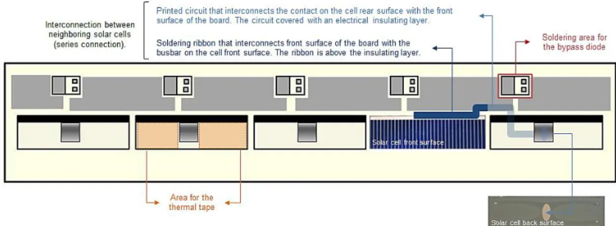
2.3.1. Interconnection 46
2.3.2. Preliminary design of the sub-receiver 48
2.3.3. First prototype 49 2.3.4. Second prototype 50 2.3.5. Final prototype 52 2.4. On-field demonstration 53 2.4.1. Sub-receiver 53 2.5. Conclusions 54 References 54
Chapter 3 – Thermal model of HSun
3.1. Experimental characterization 57
3.1.1. Experimental setup 57
3.1.2. Temperature of the solar cell 59
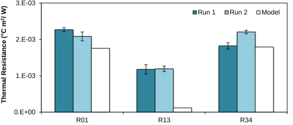
3.1.3. Thermal resistance 60
3.1.4. Experimental results 61
3.2. Validation of the CFD-FEA model 62
3.3. CFD-FEA model for the HSun receiver 64
3.3.1. Model development 64
3.3.2. Simulation results 67
3.4. Conclusions 68
References 68
Chapter 4 – Modelling CPV silicon solar cells
4.1. Introduction 69
4.1.1. Review of state of the art 70
4.2. Model 74
4.3. Cell design 74
4.3.1. Electric circuit 75
4.3.2. Current source 76
4.3.3. Diode 77
4.3.4. Series resistance components 78
4.3.5. Model dynamics 79
4.4. Conclusions 79
References 80
Chapter 5 – Model implementation and sensitivity analysis
5.1. Case study solar cell 83
5.1.1. Series resistance components 84
5.1.1.1. Measurement of the front busbar resistance 84 5.1.1.2. Measurement of the front finger resistance 84 5.1.1.3. Measurement of the contact and emitter sheet resistance 85
5.2. Simulation results for STC 88
5.3. Sensitivity analysis 89
5.3.1. Irradiance 89
5.3.2. Diode ideality factor 89
5.3.3. Series resistance components 90
5.3.4. Shunt resistance 91
5.4. Conclusions 91
References 91
Chapter 6 – Validation of solar cell electric model
6.1. Introduction 93
6.2. Validation at STC 94
6.3. Validation for homogenous profiles 94
6.3.2. High intensity illumination and temperature 96
6.4. Validation for inhomogeneous profiles 96
6.4.1. Irradiation 96
6.4.2. Temperature 98
6.5. Conclusions 100
References 101
Chapter 7 – Case studies
7.1. Comparison with standard model regarding irradiation 103
7.1.1. High irradiation 104
7.1.2. Inhomogeneous irradiation 104
7.1.2.1. Influence of peak location 105
7.1.2.2. Influence of non-uniformity 106
7.1.2.3. Influence of peak intensity 106
7.2. Comparison with standard model regarding temperature 107
7.2.1. Inhomogeneous temperature 108
7.2.1.1. Influence of peak location 108
7.2.1.2. Influence of non-uniformity 109
7.2.1.3. Influence of peak intensity 109
7.3. Model implementation for optimization of HSun technology 110 7.4. Optimization of the cell’s front grid contact 112
7.5. Conclusions 114
PART II
Introductory Note
119Chapter 1 – Ageing of DoubleSun system
1.1. Introduction 121
1.2. Methods 122
1.2.1. Outdoor exposure test 123
1.2.2. Ultraviolet conditioning test 123
1.2.3. Off-axis beam test 124
1.3. Results 124
1.3.1. Outdoor exposure test 124
1.3.2. Ultraviolet conditioning test 125
1.3.3. Off-axis beam test 125
1.4. Conclusions 126
References 126
Chapter 2 – DoubleSun performance across mainland Portugal
2.1. Introduction 127 2.2. Case study 127 2.3. Systems performance 129 2.3.1. Annual energy 129 2.3.2. Output power 130 2.3.3. Concentration coefficients 132 2.3.3.1. Resource availability 132
2.3.3.2. Energy increase due to tracking 133
2.3.3.3. Energy increase due to mirrors 133
2.3.3.4. Concentration coefficient 134
2.4. Challenges faced by on-field systems 134
References 135
Chapter 3 – Photovoltaic potencial in Terceira Island, Azores
3.1. Introduction 137
3.2. Resource characterization 138
3.3. Results 139
3.4. Conclusions 141
References 141
Chapter 4 – Levelized cost of electricity
4.1. Introduction 143
4.2. LCoE model and assumptions 143
4.2.1. Capacity costs 143 4.2.2. Annual costs 144 4.2.3. Annual energy 145 4.2.4. LCoE 145 4.3. Results 146 4.3.1. Capacity costs 146 4.3.2. LCoE 147
4.3.3. Effect of modules cost on the systems LCoE 147 4.4. Optimal concentration level for the HSun technology 148
4.4.1. Modifications on the LCoE model 149
4.4.2. LCoE for the HSun technology 150
4.5. Conclusions 151
References 152
Conclusions
153Annexes
List of Figures
PART I
Chapter 1 - Introduction
Fig. 1.1 - The principle of CPV optics using lens (on the left) and mirrors (on the right). 3 Fig. 1.2 - Global PV module price learning curve for c-Si wafer based and CdTe modules,
1979-2015. Source: (IRENA 2012). 5
Fig. 1.3 - Residential PV price parity (size of bubbles refers to market size). Notice that the LCoE is based on 6% weighted average cost of capital, 0.7%/year module degradation, 1% capex as Operation and Maintenance (O&M) annually. $3.01/W capex assumed for 2012, $2/W for 2015. Source: (Chase 2012).
5
Fig. 1.4 - Terms used for CPV ((IEC) 2007). 8
Fig. 1.5 - Criteria used in CPV classification. 8
Fig. 1.6 - Distribution of the CPV systems developed by 100 companies (Annex A, Table A.1)
according to the systems’s concentration factor. 9
Fig. 1.7 - Distribution of the CPV systems developed by 100 companies (Annex A, Table A.1)
according to the systems’ optics design. 10
Fig. 1.8 - Fresnel lens configuration: a) point-focus lens showing a typical ray hitting the circular active area of the solar cell; b) linear, or one-axis, lens focusing on a line of solar cells in a string; and c) domed linear lens. Source: (Antonio Luque & Hegedus 2003).
11
Fig. 1.9 - Reflective concentrator configurations. a) Reflective paraboloid, or dish, focusing on a cell array. b) Linear parabolic trough focusing on a line of cells. Source: (Antonio Luque & Hegedus 2003).
12
Fig. 1.10 - Example of a static concentrator configuration. A bifacial cell is mounted in a reflective CPC-like trough that is filled with liquid dielectric. Source: (Antonio Luque & Hegedus 2003). 12 Fig. 1.11 - Distribution of the CPV systems developed by 100 companies (Annex A, Table A.1) according to the solar cells technology they integrate. 13 Fig. 1.12 - Efficiency evolution of the best research cells worldwide from 1976 up top 2012 by technology type. Efficiencies determined by certified agencies/laboratories. Source: (L.L. Kazmerski 2012)
14
Fig. 1.13 - SunPower A-300 solar cell. Source: (Lawrence L. Kazmerski 2006). 15 Fig. 1.14 - MWT solar cell: a) structure of the cell (Glunz 2007) and b) picture of a highly efficient industrially feasible MWT silicon solar cell (Fellmeth et al. 2010). 15 Fig. 1.15 - Schematic drawing of an EWT solar cell of Advent Solar. Source: (Glunz 2007). 16 Fig. 1.16 - Schematic of sliver solar cells process and cell structure. Source: (Andrew Blakers et al.
2006). 17
Fig. 1.18 - Distribution of the CPV systems developed by 100 companies (Annex A, Table A.1)
regarding the type of tracking. 19
Fig. 1.19 - Two-axis tracking configurations: a) Two-axis tracker with elevation and azimuth tracking mounted on a pedestal. b) tilt tracking arrangement using central torque tube. c) Roll-tilt tracking arrangement using box frame. d) Turntable two-axis tracker. Source: (Antonio Luque & Hegedus 2003).
20
Fig. 1.20 - One-axis tracking configurations: a) One-axis horizontal tracker with reflective trough; b) One-axis polar axis tracker with reflective trough. Source: (Antonio Luque & Hegedus 2003). 21 Fig. 1.21 - EUCLIDES III concentrator a) installed at Stuttgard (Germany), including two arrays for the 24X and 12X concentration levels and b) detail of the final receiver of the EUCLIDES III, including the cells, the heat sink and the secondary mirrors. Source: (Marta Vivar et al. 2011).
22
Fig. 1.22 - HCPV system developed by Amonix: a) schematic of the system and b) photograph of the system installed in Arizona Public Service’s Solar Test and Research (STAR) facility in 1994. Source: (V Garboushian et al. 1996).
23
Fig. 1.23 - Concentration photovoltaic (CPV) system developed by Solar Systems Australian company: a) Power station of 190kWp in Hermannsburg; b) detail of the MJ 33 kWp receiver. Source: (Pierre J. Verlinden 2006).
23
Fig. 1.24 - Archimedes system: a) principle scheme of the structure and b) frontal view. Source:
(Klotz et al. 2001). 24
Fig. 1.25 - Combined Heat and Power System (CHAPS) at Australian National University: a) picture of the system; and b) schematic of a cross-section of the receiver with the cells and cooling system. Source: (M. Vivar et al. 2010).
24
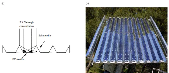
Fig. 1.26 - Whitfield system: a) Whitfield system, b) components of a V-trough carrying the cell; and c) close-up of the illumination spot on the cell also showing a bypass diode. Sources: (Bentley et al. n.d.).
25
Chapter 2 – The HSun system
Fig. 2.1 - HSun module mounted on a two-axis tracking system. Courtesy of: WS Energia S.A. 31
Fig. 2.2 - Schematic of a PV solar cell. 33
Fig. 2.3 - Standard electric single-diode model for a solar cell. 33 Fig. 2.4 - Current-Voltage (I-V) curve and its main parameters for a solar cell. 34 Fig. 2.5 - Estimated power loss (Ploss) and efficiency (ε) as a function of the concentration level.
The dashed line represents the efficiency without considering the Joule losses. 36 Fig. 2.6 - Scanning Electron Microscope (SEM) image of a finger contact for a) NaREC and b)
Solartec solar cells. 38
Fig. 2.7 - NaREC solar cell and detail of the busbar. 38 Fig. 2.8 - Solartec solar cell: a) front surface and b) back surface. 39 Fig. 2.9 - Current density - Voltage (J-V) curves measured under STC for: a) NaREC and b)
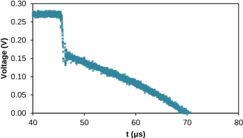
Fig. 2.10 - Schematic of a) setup used in the OCVD method and b) expected V(t) curve. Source:
(D. K. Schroder 2006). 41
Fig. 2.11 - Curves obtained through the OCVD method for the NaREC solar cell when a current of
1.5 A is imposed. 42
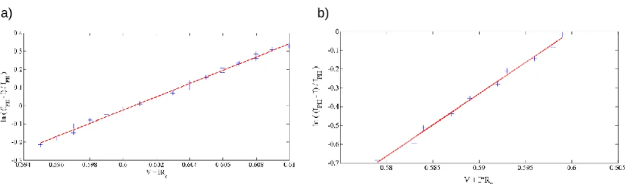
Fig. 2.12 - Semi-logarithmic plot for the NaREC and Solartec cells, respectively. 43 Fig. 2.13 - Measured a) I-V curves for the NaREC solar cells at 1000 W/m2 and different temperatures: 25, 30, 40, 50 and 60°C. Through the Voc and Isc registered in these curves, the
thermal coefficients for the b) Voc and c) Isc were calculated.
45
Fig. 2.14 - Measured a) I-V curves for the Solartec solar cells at 1000 W/m2 and different temperatures: 25, 30, 40, 50 and 60°C. Through the Voc and Isc registered in these curves, the
thermal coefficients for the b) Voc and c) Isc were calculated.
46
Fig. 2.15 - Soldering process of a ribbon on the solar cell busbar: a) positioning of the solar cell into the aluminium base; b) pen flux to apply some flux on the cell’s busbar in order to facilitate solder adhesion between the cell and the ribbon; and c) positioning and soldering the tab to the busbar through a soldering iron.
47
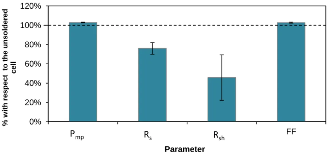
Fig. 2.16 - Maximum power (Pmp), Series resistance (Rs), Shunt resistance (Rsh) and Fill Factor
(FF) of the soldered cell as a percentage of the value obtained for the unsoldered cell. 48 Fig. 2.17 - Schematic of the first sub-receiver prototype. The cells are represented by the blue rectangle and the interconnection between them are represented by the grey areas (when are designed in the board) and the red tabs (when soldered to the cell).
48
Fig. 2.18 - Electrical scheme of the interconnection between solar cells in the first sub-receiver
prototype. 49
Fig. 2.19 - First receiver prototype with two series connected cells on the centre and two bypass
diodes on the borders. 50
Fig. 2.20 - Printed circuit board (PCB) and schematic of the components placement and
interconnection. 51
Fig. 2.21 - Finished sub-receiver including the PCB with the bypass diodes, and the soldered ribbon interconnecting each cell to the neighbouring cell in a series connection. 51 Fig. 2.22 - Distribution of the sub-receivers within a certain range of Pmp: a) before and b) after the
re-soldering process. 52
Fig. 2.23 - Distribution of sub-receivers that are within a certain range of Pmp: a) before and b) after
the re-soldering process. 52
Fig. 2.24 - Sub-receiver mounted for on-field demonstration. Source: (Ramos 2011). 53 Fig. 2.25 - Short-circuit current (on the left) and open-circuit voltage (on the right) measured for each solar cell (red bars) and for the sub-receiver (blue bar) under outdoor conditions: 800W/m2 of irradiation and 30.5°C of ambient temperature, normalized to the Isc and Voc estimated expected for
the solar cell under such conditions (black dashed lines). Source: (Ramos 2011)
53
Chapter 3 – Thermal model of HSun
Fig. 3.2 - Solar simulador: a) build at SESUL laboratory; b) schematic representation of the solar simulator; and c) detail of the sample holder integrated in the solar simulator. 58 Fig. 3.3 - Schematic of the experimental apparatus for the measurement of the temperature of each
material. 59
Fig. 3.4- Equivalent thermal circuit of the receiver. 61 Fig. 3.5 - Cell temperature (squares) estimated by the Voc and temperature measured for material 2
(circles), material 3 (lozenges) and the sample holder (asterisk) during Run 1 (darker colours) and Run 2 (lighter colours).
62
Fig. 3.6 - Temperatures obtained experimentally (Run 1 and Run 2) and by the model simulation. 63 Fig. 3.7 - Thermal resistances estimated using the temperatures obtained experimentally and by the
simulation. 63
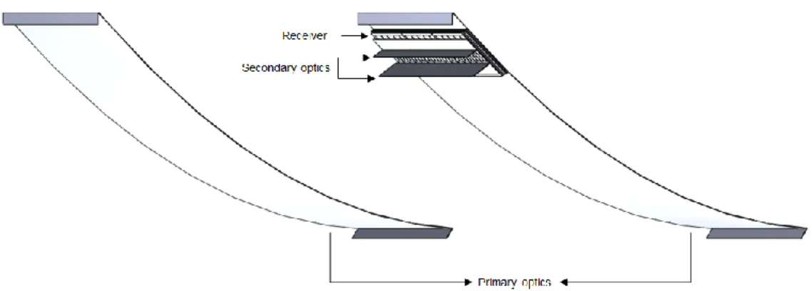
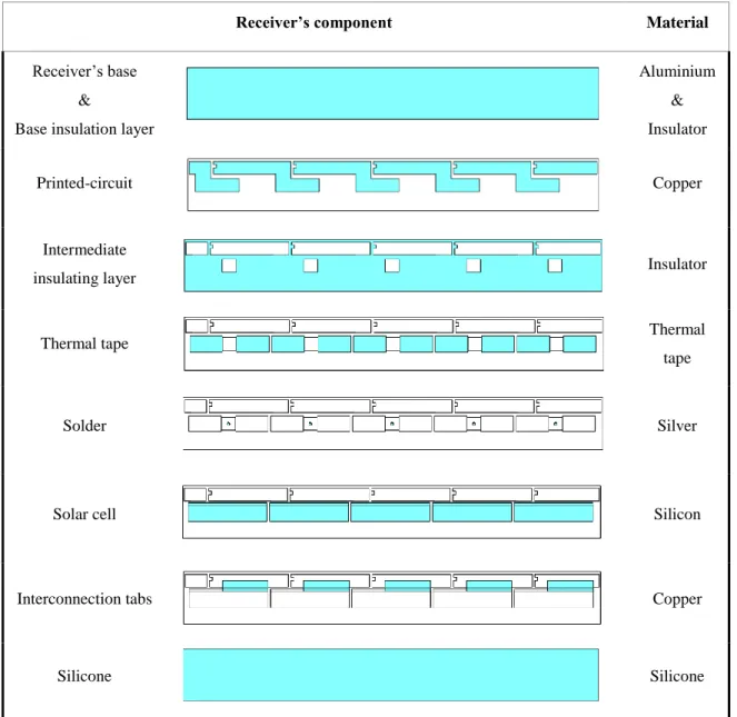
Fig. 3.8 - Top view of the temperature distribution on the solar cell for a simulation of 19 suns: rear surface of material 3 at 42ºC and an ambient temperature of 25ºC. 64 Fig. 3.9 - HSun structure considered for case study of the receiver thermal behaviour. 64 Fig. 3.10 - Schematic of the receiver layers (and the corresponding materials) from bottom to top. 66 Fig. 3.11 - Irradiation profile (suns) across the solar cell width (only considering the distance between the busbar and the opposite edge of the cell). 66 Fig. 3.12 - Temperature profile on half of the receiver for: a) the case in which the receiver is 1.5 mm away from the primary optics behind it; and b) the case in which receiver’s back surface is thermally connected to the back surface of the primary optics behind it. In the latter case it is also shown a detail (b1) of the temperature profile across three solar cells.
67
Chapter 4 – Modelling CPV silicon solar cells
Fig. 4.1 - Lumped resistance model for a solar cell. 70 Fig. 4.2 - Decrease in a) open-circuit voltage (Voc) and b) efficiency (ε) against peak illumination
ratio. Each result is identified by the first author of the paper. 73 Fig. 4.3 - Design of: a) the solar cell considered as case study; b) a solar cell element; and c) the equivalent electric circuit of a solar cell element. 75 Fig. 4.4 - Equivalent electric circuit for the elementary units located in: a) the semiconductor region and b) the contact region. Depending on the cell region that is being considered, Rx may
become Rf (finger) or Rb (busbar).
76
Fig. 4.5 - Flowchart of the solar cell model implemented in Matlab/Simulink. 79
Chapter 5 – Model implementation and sensitivity analysis
Fig. 5.1 - Front grid pattern of a solar cell showing the placement of the probes for a four-point
measurement of the busbar resistance. 84
Fig. 5.2 - Position of the probes for a four-point measurement of the average finger resistance on a solar cell with one busbar. Notice that in the case of one single busbar on the cell, the busbar is 85
removed from the cell to perform the measurement.
Fig. 5.3 - Front grid pattern of a slice of solar cell without busbars showing the placement of the probes for a four-point measurement of the contact and emitter sheet resistances. 85 Fig. 5.4 - Plot for extracting the contact and emitter sheet resistances. 86 Fig. 5.5 - I-V curve measured and modelled under STC conditions. 88 Fig. 5.6 - Sensitivity of each parameter (Isc, Voc and Pmp) with respect to variations on the
irradiance. 89
Fig. 5.7 - Coefficients for: a) percentage variation of Voc and b) percentage variation of Pmp with
respect to the percentage variation of n plotted against the concentration/temperature levels for different temperature/concentration, respectively.
90
Fig. 5.8 - Power loss versus series resistance components increase of 25%, 50% and 75.8% for: a)
1 sun and b) 15 suns. 90
Fig. 5.9 - Power loss versus variation in shunt resistance (Rsh) for a concentration level of 1 sun
(light blue diamond markers) and 15 suns (dark blue squared markers). 91
Chapter 6 – Validation of the solar cell electric model
Fig. 6.1 - Modelled (solid line) and experimental (squared markers) current-voltage (dark blue) and power-voltage (light blue) curves for the solar cell in study under Standard Test Conditions (STC). 94 Fig. 6.2 - Modelled versus measured values for a) short-circuit current (dark blue squared markers) and maximum power point (light blue triangle markers) and b) open-circuit voltage (blue circle markers) for a solar cell homogeneously illuminated under different irradiance values within a range between 1 and 30 suns and at 25°C.
95
Fig. 6.3 - Modelled versus measured value of Voc for a cell under 1 sun (light blue squared
markers), 11 suns (medium blue triangle markers) and 19 suns (dark blue circle markers) for different solar cell temperatures. The Voc values are normalized to the Voc modelled and measured,
respectively, for the same irradiation conditions at 25°C.
96
Fig. 6.4 - Illumination profiles for a) stepwise illumination and b) Gaussian profiles. 98 Fig. 6.5 - Experimentally versus modelled results obtained for maximum power point for each illumination profile. Notice that both experimental and modelled results are normalized with respect to the results under STC.
97
Fig. 6.6 - Experimentally versus modelled results obtained for maximum power point for each illumination profile. Notice that both experimental and modelled results are normalized with respect to the homogeneous irradiation case at 15 suns and 25ºC.
98
Fig. 6.7 - Temperature profile (in °C) obtained for: a) the sample holder and b) the solar cell when
placed on it. 98
Fig. 6.8 – Sample holder. 99
Fig. 6.9 - Open-circuit voltage (Voc) measured (markers) and modelled (solid lines) for a solar cell
with i) homogeneous temperature distribution (black markers and line); ii) a temperature profile whose maximum value is on the busbar (red markers and line); and iii) a temperature profile whose minimum value is on the busbar (blue markers and line). Notice that the dashed lines correspond to the trendline of the measured data.
Chapter 7 – Case studies
Fig. 7.1 - Current estimated by the distributed model versus the current estimated by the standard model for the same voltage at STC. The red dot represents the Impp point.
103
Fig. 7.2 - Maximum power point (Pmp), estimated by the conventional lumped model (dashed grey
line) and the distributed model (dashed black line) for different concentration levels. The experimental values are also presented (blue squared markers).
104
Fig. 7.3 – Power loss of a solar cell inhomogeneously illuminated with respect to the power at homogeneous irradiation distribution with an average of 29.2 suns. In the cell schematic the black bar represents the cell busbar and the pallet of shades is illustrative of the highly illuminated (white) and lower illuminated (dark grey) regions.
105
Fig. 7.4 - Maximum power point (Pmp) in as a percentage of the Pmp obtained for the homogeneous
illumination case with the same average illumination versus the parameter of irradiation inhomogeneity, r.
106
Fig. 7.5 - Power loss of the inhomogeneous illuminated cells with respect to the homogeneously illuminated with the same average irradiation plotted against the average irradiation on the cell. 107 Fig. 7.6 - Maximum power point (Pmp) estimated by the conventional lumped model (cross markers
with dashed black line) and the distributed model (squared markers with dashed light blue line) for different temperatures.
107
Fig. 7.7 - Power loss of a solar cell when subjected to a non-uniform temperature profile with respect to the power at homogeneous temperature distribution with the same average (49.6°C). Notice that in the cell schematic, the black bar represents the cell busbar and the pallet of shades is illustrative of the warmest (red) and colder (white) regions.
108
Fig. 7.8 - Open-circuit voltage obtained for a solar cell under different temperature profiles. The results are shown against the t parameter and are normalised to the Voc obtained at STC.
109
Fig. 7.9 - Open circuit voltage (Voc) obtained for the solar cell under homogeneous (black solid line
with diamond markers) and inhomogeneous (red dashed lines with square markers) temperature profiles.
109
Fig. 7.10 – Irradiation profile along the cell width: i) predicted by the Ray Tracing software (black markers) and ii) interpolation to the data (red line). 110 Fig. 7.11 – Temperature profile for a solar cell located at the edge of the receiver. The black markers correspond to the points obtained through CFD-FEA simulations in Solidworks while the coloured surface corresponds to the interpolation performed to such points.
111
Fig. 7.12 – Curves obtained for a) Current-Voltage (I-V) and b) Power-Voltage (P-V) for a cell at the middle (light blue line) and a cell at the edge of the receiver (dark blue line). The black dashed line represents an I-V curve for a solar under homogeneous irradiation and temperature for the average values found within the HSun cells.
112
Fig. 7.13 - Efficiency obtained for each solar cell design with respect to the efficiency obtained for the original cell design plotted against the number of fingers. The solar cell under analysis presents a radiation and temperature profiles similar to the solar cell located at the edge of the HSun receiver. The red squared marker corresponds to the optimum number of fingers while the white squared marker corresponds to the original solar cell.
113
Fig. 7.14 – Current-Voltage (I-V) curves obtained for each solar cell design (i.e. different number of fingers) when considering the cell located at the edge of the HSun receiver. 113
PART II
Chapter 1 – Ageing of DoubleSun® system
Fig. 1.1 – DoubleSun® system installed at WS Energia laboratory in Oeiras, Portugal (38º41’50’’N, 9º18’30’’W). Source: WS Energia S.A. 122
Fig. 1.2 - Prototype similar to DoubleSun® technology. 124 Fig. 1.3 - Current-Voltage (I-V) curve measured for the module under 1sun (dark blue squared markers) and 1.85 suns (light blue triangle markers) a) before UV exposure and b) after UV exposure. Notice the decrease of Isc in case b) when the module is integrated in the CPV system
(C=1.85).
125
Chapter 2 – DoubleSun® performance across mainland Portugal
Fig. 2.1 - Percentage distribution of the 110 PV systems across mainland Portugal. 128 Fig. 2.2 - Geographical distribution through mainland Portugal of the PV systems in analysis: DoubleSun® (red dots) and flat plate (white dots). 128 Fig. 2.3 – Accumulated energy produced by the DoubleSun® (squared markers) and a flat-plate (triangle markers) system from July 2009 to June 2010. In the up left corner the average annual energy produced by each system during the period under analysis is presented with respect to the flat-plate system annual energy.
129
Fig. 2.4 - Energy produced by month for: a) DoubleSun® and b) flat-plate systems installed across
mainland Portugal. 130
Fig. 2.5 - AC power of the DoubleSun® (blue) and Flat-plate systems (red) registered during a clear day (solid lines) and daily average (dashed lines) for: a) December 2009 and b) June 2010. The systems were installed in Lisbon.
131
Fig. 2.6 - Annual average of δ and δ* for different locations in Portugal mainland. 132 Fig. 2.7 - Annual average of γ for different locations in Portugal mainland. 133 Fig. 2.8 - Annual average of α and α* for different locations in Portugal mainland. 134 Fig. 2.9 - Annual average of R and R* for different locations in Portugal mainland. 134
Chapter 3 – Photovoltaic potential in Terceira Island, Azores
Fig. 3.1 - Group of Azores islands. Source: (Fans n.d.). 137 Fig. 3.2 - Daily profile of: a) global, b) direct, and c) diffuse irradiance (W/m2) measured during
2009 at Angra do Heroísmo, in Terceira Island. 138
Fig. 3.3 - Daily profile of the ambient temperature (°C) measured during 2009, in Angra do
Heroísmo. 139
Fig. 3.4 - Ratio of the AC power between: a) 2-axes tracking system and a flat plate system; b) the DoubleSun® system and a tracking system; and c) the DoubleSun® system and a flat-plate system. 140
Fig. 3.5 - Energy produced by a 2 axes tracking system and by a DoubleSun system normalized to
the energy produced by a flat-plate system. 140
Fig. 3.6 - Expected accumulated energy (kWh/kWp) produced by the flat-plate system, 2-axes tracking system and the DoubleSun® system during 2009 in Angra do Heroismo. 141
Chapter 4 – Levelized cost of electricity
Fig. 4.1 - Energy (kWh/kWp) produced by each system configuration during its lifetime. 146 Fig. 4.2 - Cost of the main elements of each system as a percentage of the total cost of the system. 147 Fig. 4.3 - LCoE for the DoubleSun, two-axis tracker, one-axis tracker and the conventional
flat-plate system. 148
Fig. 4.4 - LCoE of the flat-plate system with respect to the LCoE of: i) a DoubleSun® system (orange line); ii) a two-axis tracking system (dark blue line); and iii) a one-axis tracking system (light blue line).
149
Fig. 4.5 - Levelized Cost of Electricity (LCoE) estimated for the HSun technology at different
List of Tables
PART I
Chapter 2 - The HSun system
Table 2.1 - Solar cell dimensions. 39
Table 2.2 - Series resistance of the NaREC and Solartec solar cells estimated by different
methods. 42
Table 2.3 - Electrical parameters obtained through the I-V curve measured under STC of the
NaREC and Solartec solar cells. 43
Table 2.4 - Thermal coefficients for the short-circuit current (ki) and open-circuit voltage (kv)
estimated for the NaREC and Solartec solar cells. 46
Chapter 3 - Thermal model of HSun
Table 3.1 – Materials associated to the HSun receiver’s case study used in the CFD-FEA. 65
Chapter 4 - Modelling CPV silicon solar cells
Table 4.1 - Resistors developed for the model. 78
Chapter 5 - Model implementation and sensitivity analysis
Table 5.1 – Model input parameters. 83
Table 5.2 - Resistivities found in the literature. 87 Table 5.3 - Resistivities measured for the NaREC and Solartec cells. 88
Chapter 6 - Validation of the solar cell electric model
Table 6.1 - Experimentally measured solar cell parameters (dimensions, electric, thermal coefficients and resistances) relevant for the implementation of the model. 94
Chapter 7 - Case studies
Table 7.1 – Minimum (Tmin), maximum (Tmax) and average (Tavg) temperature for the solar cell
PART II
Chapter 1 - Ageing of DoubleSun® system
Table 1.1 - Typical electrical parameters of the modules used in the outdoor exposure test. 123 Table 1.2 - Electrical parameters of the module used in UV conditioning test. 124 Table 1.3 - Electrical parameters of the module before and after 6 months of outdoor exposure. 125
Chapter 4 - Levelized cost of electricity
Table 4.1 - Cost (€/Wp) of the components and installation of each PV system considered in the
present analysis (SOURCE: WS Energia). 145
List of Variables
A Unit area in Simulink Aactive Active area
AT Tracking area
C Concentration level
C0 Concentration of 1 sun, i.e. 1000 W/m2
CI Installation cost
CM Modules cost
CO Optics cost
CO&M Operation and maintenance cost
Copt Optimum concentration level
CT Tracker cost
d Space between fingers dr Discount rate
dxe Length of the elementary emitter unit
dxf Length of the elementary finger unit
dy Emiter unit width f Number of elements FF Fillfactor
g Degradation rate
I Current
I0 Reverse saturation current
ic ratio between direct irradiation and normal irradiation
ID Diffusion diode current
Idiode Diode current
Iimposed Current imposed in the cell when performing OCVD method
Impp Current at maximum power point
Iph Photogenerated current
Isc Short-circuit current
Ish Current through the shunt resistor
j Number of fingers
Jsc Short-circuit current density
Jsc(STC) Short-circuit current density under STC
k Boltzmann constant (1.380 x 10⁻²³J/K) ki Thermal coefficient for current
kV Thermal coefficient for voltage
n Ideal factor of the diode Pin Irradiance falling on the cell
PIR Peak Illumination Ratio Ploss Power loss
Pmp Maximum power point
Psystem Power of the system
q Electron charge (1.602 x 10⁻¹⁹ C) Q Radiation that falls on the cell Qn Energy output per installed power
r Parameter that refers to the degree of illumination inhomogeneity on the cell R Concentration coefficient
Ravg Average irradiance on the cell
Rbulk Bulk resistor
Rc Contact resistor
RCH Characteristic resistance
Re Emitter resistor
Rf Finger resistor
Rmax Maximum irradiance on the cell
Rmin Minimum irradiance on the cell
Rs Series resistance
rS Normalized series resistance
Rsh Shunt resistance
T Temperature
t Parameter that refers to the degree of temperature inhomogeneity on the cell T0 Ambient temperature, 25°C
Tavg Average temperature on the cell
TLCC Total life cycle cost
Tmax Maximum temperature on the cell
Tmin Minimum temperature on the cell
TSTC Ambient temperature, 25°C
V Voltage
Vmpp Voltage at maximum power point
Voc Open-circuit voltage
Voc(STC) Open-circuit voltage at Standard Test Conditions (STC)
VT Thermal voltage
W Cell width y Year of operation Y Period under analysis Z Busbar/Finger thickness
α parameter to evaluate the energy increase due to the mirrors β Busbar width
γ Parameter to evaluate the energy increase due to tracking δ Parameter to evaluate the resource availability
ΔR Difference between the maximum and minimum irradiance values ΔT Difference between the maximum and minimum temperature values ΔV Voltage drop due to series resistance
ε
Efficiencyεa Efficiency of the active area
εo Optical efficiency
εsystem Efficiency of the system
ρc Contact resistivity ρe Emitter resistivity
List of Acronyms
ANU Australian National University BOS Balance of system
CdTe Cadmium Telluride
CFD-FEA Computational Fluid Dynamics - Finite Element Analysis CHAPS Combined Heat And Power System
CPV Concentration Photovoltaic c-Si Crystalline-Silicon
DNI Direct Normal Irradiation EWT Emitter-Wrap-Through
HCPV High Concentration Photovoltaic Systems
IES-UPM Instituto de Energia Solar - Universidad Politécnica de Madrid
ISE Institut für Solare Energiesysteme I-V curve Current-Voltage curve
LCoE Levelized Cost of Electricity
LCPV Low Concentration Photovoltaic Systems LGBC Laser Grooved Buried Contact
MCPV Medium Concentration Photovoltaic Systems
MJ Multi-junction
MWT Metal-Wrap-Through
NaREC National Renewable Energy Centre (UK) OCVD Open Circuit Voltage Decay
PC Point-Contact
PCB Printed Circuit Board
PV Photovoltaic
P-V curve Power-Voltage curve
PVGIS Photovoltaic Geographical Information Systems SEM Scanning Electron Microscope
SESUL Sustainable Energy Systems of University of Lisbon
Si Silicon
SPICE Simulated Program with Integrated Circuits Emphasis STC Standard Test Conditions (25°C, 1000 W/m2, AM1.5) SUPSI-ISAAC University of Aplied Sciences and Arts of Switzerland ZSW Zentrum fur Sonnenenergieund Wassertoff-Forschung
Chapter 1 Concentration Photovoltaics
This chapter briefly reviews the history of concentration photovoltaics (CPV) and discusses the most relevant challenges and opportunities for its development. Then, it describes the main terms, concepts and definitions used in the field and also in this work. After, a brief overview of the classification of each CPV component and its options is carried out. Finally, a review of the most noticeable CPV systems experiences is presented.
1.1.
Introduction
Photovoltaic (PV) technology is a clean and inexhaustible solution to convert sunlight energy into electrical energy (Antonio Luque & Hegedus 2003; Nelson 2003). The growing interest on this technology has significantly increased in the 1970s with the oil crisis. Since the early days of terrestrial PV application, and given that the available solar cells (basic converter unit of a PV system) were perceived to be too expensive, the use of concentrating sunlight has arisen as a possible shortcut to significantly reduce the cost of PV electricity (Swanson 2000; A. Luque et al. 2006; A. Bett et al. 2006; A. Luque & Andreev 2007). This concept is known as concentrator photovoltaic technology and consists in redirecting the sunlight onto a small solar cell area through optical devices, as illustrated in Fig. 1.1. Thus, the area of the PV cell is reduced while, at the same time, the light intensity on the device increases by the same ratio. Of course, the expectation is that the replacement of the expensive PV solar cells by less expensive optical material (lenses and/or mirrors) may lead to some savings in system costs (A. Bett et al. 2006; Antonio Luque & Hegedus 2003; A. Luque et al. 2006; A. W. Bett et al. 2007; Reis, Pina, et al. 2011).
Fig. 1.1 - The principle of CPV optics using lens (on the left) and mirrors (on the right).
Research on CPV systems began in 1975 and its development was encouraged by the US “Concentrator Program”, which arose due to the prediction of the increased costs of fossil fuels in the aftermath of the 70s’ oil crises. CPV was mainly conceived for large power plants, aiming to produce
large amounts of renewable energy and compete with conventional fossil fuel plants (A. Luque et al. 2006; Swanson 2000; A. Luque & Andreev 2007). Within this program, the first concentrator prototype was developed at Sandia National Laboratories of Albuquerque in the mid 1976. This prototype was a 40x concentrator, making use of silicon solar cells and Fresnel lenses mounted on a two-axis tracking system (Burgess & Pritchard 1978). Shortly afterwards, several prototypes were developed in Europe. They were all similar to the one made by Sandia Labs.
However, the electricity market changed in a somewhat unexpected direction. Global politics and the discovery of new oil sources kept electricity prices of the mature fossil fuel plants at a very low level. Since the concentrator programs were initially conceived to construct CPV for large power plants, i.e. to compete with fossil fuel generators, most of them were suspended in the face of the unexpected abundant fossil fuel supply. This situation has slowed down the development of CPV systems. In the mid of 1980s, R&D on concentrators faded although some groups maintained activity (A. Luque et al. 2006).
In the niche market of small remote loads used for grid extension applications (e.g. small amount of electricity to telecommunication stations) flat-plate PV emerged as an important and viable power source. CPV however, due to the need to be mounted on movable structures to track the sun, is particularly unsuitable for these applications and has never gained a significant market share.
In the meantime, the new paradigm of sustainability, the need to confront global warming and the external costs associated with pollution became the driving force for PV development. Subsidized grid-connected market of a few kWp has emerged more recently in many developed countries. In these applications CPV also played a minor role in PV market for more than 25 years (A. Luque et al. 2006; Swanson 2000; A. W. Bett et al. 2007). The PV systems in the subsidized grid connected market were often mounted on the roof or integrated in facades (reducing some of the installation cost) which again are less suitable for CPV (A. Luque et al. 2006; Antonio Luque & Hegedus 2003; Swanson 2000; A. W. Bett et al. 2007). However, we may found some CPV systems installed under feed-in tariff schemes in places where extensive grounds are available (Reis, Silva, et al. 2011).
This brief historic overview emphasises the main barriers that CPV has faced when trying to gain market acceptance. In spite of all these challenges, it should also be noticed that the development of CPV technology has contributed to some advances in other areas. One example of such contribution is the improvement of the efficiency of solar cells. The high power density of CPV allows the use of cells with higher cost per unit area. Thus, many designs were developed specifically for concentration applications. Some of these concepts have been successfully applied to one-sun solar cells (Swanson 2000).
Another technological development which has spill over from CPV to conventional PV is tracker technology. Standard modules mounted on tracking structures may lead to higher yields that overcome the extra cost of the trackers (Reis, Pina, et al. 2011), in particular in locations with high direct insolation.
An additional side effect of the development of CPV was the knowledge acquired about the availability of direct normal irradiation (DNI). The boost of energy yield on CPV systems is mostly related with the amount of direct sunlight (radiation that falls on Earth without being scattered by haze, clouds, etc). In the early days of the Concentrator Program it was feared that the percentage of such radiation was considerably less than the solar resource available for flat-plate systems, which make use of global radiation. However, it was found that in many regions of good solar resource, the annual energy
available to a two-axis tracking concentrator is actually greater than the global radiation resource available to flat-plate systems (Swanson 2000; Reis, Wemans, et al. 2011; Reis, Silva, et al. 2011).
During the mid 2000s, and in spite of very significant political and economic support, the cost reduction of conventional flat plate PV was perceived to be too slow and therefore a lot of effort, and research funding, both public and private, was re-directed to CPV, which offered the promise of a faster learning curve. Examples are large scale CPV demonstration program in the region of Castilla La Mancha, Spain, and in Portugal, as well as numerous start-ups dedicated to CPV that emerged in the past 5-10 years (A. Luque & Andreev 2007; Brad Hines 2007).
Today, the world is in great need of a change in the way that energy is generated. On one hand, most governments have in their agenda the concerns about greenhouse gas emissions and climate change while, on the other hand, the rising prices of energy and fossil fuels and the Fukushima nuclear disaster have led to increasing interest in renewable energy sources in general, and solar in particular (Brad Hines 2007). The PV industry is now growing to a scale that it can play a measurable contribution of Europe’s electricity mix, producing 2% of the demand in EU and roughly 4% of the peak demand (Masson et al. 2012). The character of the industry is undergoing a significant change, with abrupt cost reductions in silicon module in 2011 and 2012 (Fig. 1.2), and PV markets approaching competitiveness in the electricity sector towards “grid parity” (Fig. 1.3) (Kurtz 2012; Masson et al. 2012).
Fig. 1.2 - Global PV module price learning curve for c-Si wafer based and CdTe modules, 1979-2015. Source: (IRENA 2012).
Fig. 1.3 - Residential PV price parity (size of bubbles refers to market size). Notice that the LCoE is based on 6% weighted average cost of capital, 0.7%/year module degradation, 1% capex as Operation and Maintenance (O&M) annually. $3.01/W capex assumed for 2012, $2/W for 2015. Source: (Chase 2012).
So the big question is how may CPV compete against traditional flat-plate PV and other renewable energy technologies? Many factors may be pointed out (Brad Hines 2007; A. W. Bett et al. 2007; Kurtz 2012; Cameron n.d.):
Improvements in solar cell technology: solar cell manufacturers are now delivering high efficiency solar cells above 20% for silicon and 40% for triple-junction. These high-efficient cells are affordable for CPV systems due to the reduced area requirements. This way CPV may achieve excellent amortization on system costs.
Desire for utility scale systems: one of the vectors that PV growth aims to reach is large installations that yield significant power. CPV is particularly suitable for this type of applications since large scale deployment leads to lower installation costs. In this field, CPV may have some advantage in terms of land use since for 1 GWh uses 0.9 ha of land compared to 1.6 ha for thin-film and 1.7 ha for a solar thermal power tower. However, this factor has only economic value in places where land costs have a high impact on the overall system cost such as southern Europe, Brazil or India. Still, on the path for large power plants, CPV will also compete with other renewable energy technologies such as wind, over which has the advantage of higher predictability and a wider selection of installations sites with much more energy available. Fossil fuel power plants will still play a relevant role due to competitive costs; however, these plants have a huge vulnerability to fossil fuel depletion, cost escalation and pollution directives, factors that may lead to increased prices thus helping CPV to become competitive.
Large incentive schemes are becoming less attractive: with the increasing cost reduction on silicon modules, incentives will become unnecessary to reach the market in a cost effective way, in particular in sunny regions with high conventional electricity prices. This may represent a shift on the PV market to the countries where incentive schemes are inexistent and with high availability of sun, where CPV may be a viable option.
Relatively low capital investment: the capital investment risk for CPV is distributed between its components (which are described in detail in the next section) and other suppliers; moreover the cost is reduced overall because these investments may be shared to other products that use the same materials with long-life outdoor performance demonstrated. This makes CPV investment a lower risk than from some other types of PV.
Better match between electricity production and demand: PV systems mounted on sun trackers, as it is almost compulsory for CPV systems, have increased production during the mornings and afternoons, since flat plate PV are usually installed in order to optimize production when the irradiation is higher (mid-day peak hours) ; this could be advantageous from the point of view of the electricity grid since CPV systems may deliver power in order to fulfil demand without the need for storage.
Concentrator leverage over traditional flat-plate systems: CPV systems have performance advantage in sunny areas, relative lack of sensitivity to the price of solar cells, and they use less solar cell material which may be advantageous during a time of short supply of that material.
Today, about 50 companies are active in the CPV technology field and almost 60% of them were founded in the last six years (Jäger-Waldau 2012). However, in order to achieve a relevant role in the market, the cost of CPV must be lowered. It was only recently that a number of companies started to commercialize CPV systems (A. W. Bett et al. 2007). Most recent market estimates for 2011 in the 60 MW range, and 90 MW under construction in May 2012, the market share of CPV is still small, but analysts forecast an increase to more than 500 MW globally by 2015 (Jäger-Waldau 2012).
Before reviewing the most noticeable CPV systems it is appropriate to briefly look over some relevant terms, concepts and classifications in order to facilitate the understanding of the different concepts and approaches to CPV.
1.2.
Terms and concepts
The design of CPV systems may vary a lot and may have much more complex structures than standard PV systems. A transversal definition of components, terms and concepts of CPV is stated in the IEC 62108 standard ((IEC) 2007) and are summarised below. Figure 1.4 illustrates the relationship between these different definitions:
Concentrator: term associated with photovoltaic devices that use concentrated sunlight. Concentrator optics: optical components that perform one or more of the following functions
from its input to output: increasing the light intensity, filtering the spectrum, modifying light intensity distribution, or changing light direction. Typically it consists on a lens or mirror and it may be subdivided in:
• Primary optics: device that receive sunlight directly from the sun.
• Secondary optics: device that receives concentrated or modified sunlight from another
optical device, such as primary optics or another secondary optics.
Concentrator cell: basic photovoltaic device that is used under the illumination of concentrated sunlight.
Concentrator receiver: group of one or more concentrator cells and secondary optics (if present) that accepts concentrated sunlight and incorporates the means of thermal and electric energy transfer. The receiver could be made of several sub-receivers, which consists on a smaller portion of the full-size receiver.
Concentrator module: group of receivers, optics and other related components, such as interconnection and mounting, that accepts sunlight directly from the sun. All these components are usually prefabricated as one unit, and the focus point is not field-adjustable. A module could be made of several sub-modules being this a physical standalone portion of the full-size module. Concentrator assembly: group of modules and other related components such as
interconnection and mounting, that accepts sunlight directly from the sun. All these components are usually shipped separately and need field installation, and focus point is field-adjustable. An
assembly could be made of several sub-assemblies. The sub-assembly is a physical stand-alone, smaller portion of the full-size assembly.
Fig. 1.4 - Terms used for CPV ((IEC) 2007).
1.3.
CPV configurations
There are many different CPV systems configurations. The technical solutions taken for each component may vary significantly and in the following lines we present and discuss some of the most common configurations for each component, as summarized in Fig. 1.5. Some of the most noticeable examples are also presented in the next section.
1.3.1. Concentration factor
The CPV systems may be divided into three classes, depending on the system’s concentration factor, whose most common definition is the “geometric concentration ratio”, defined as the ratio between the area of the primary optics and the active cell area (Antonio Luque & Hegedus 2003). Taking into account the concentration factor, and following Sarah Kurtz (Kurtz 2012), CPV systems may be divided in:
Low Concentration Photovoltaic (LCPV) , with a typical concentration ratio lower than 3X; Medium Concentration Photovoltaic (MCPV), for systems with a typical concentration ratio
that lies between 3X and 100X; and
High Concentration Photovoltaic (HCPV), for values of concentration higher than 400X.
It must be noticed that the range of concentration factors for each category may vary a lot, depending on the author or even the publication date. From a CPV market perspective, we found 100 companies (which are listed in Annex A, Table A.1) from which, as shown in Fig. 1.6, the majority (about 44%) develop systems with concentration levels above 400X, i.e. high concentration photovoltaic systems. Also in this figure, the less attractive concentration level seems to be below 3X, i.e. low concentration systems. Most of the LCPV systems were mainly developed between 2007 and 2008, when silicon modules were extremely expensive and, this way, the companies designed ingenious methods for making their conventional silicon modules generate more electricity. The solution of adding mirrors to enhance the irradiance falling on the modules was widely explored by private players (Kurtz 2012), as WS Energia did with the DoubleSun® technology (Reis et al. 2010). However, the sharp fall in the price of the modules (see Fig. 1.2) lead to decreasing the interest in this approach.
Fig. 1.6 - Distribution of the CPV systems developed by 100 companies (Annex A, Table A.1) according to the systems’ concentration factor.
Another common alternative measure of concentration is the intensity concentration, or “suns”, which is calculated through the division between the average intensity of the concentrated light that
3% 10% 8% 44% 35% ≤ 3X 3X - 100X 100X - 400X ≥ 400 n.a.
reaches the cells and the standard peak solar irradiance 1000 W/m2 (Antonio Luque & Hegedus 2003). Both measures are valid still it should be noticed that the latter takes into account the optical losses while the former disregard them.
1.3.2. Concentrator optics
The concentrator optics must be designed in such a way that its acceptance angle, i.e. the maximum angle at which the rays entering the optics reach the cell, admits the misalignments and tolerances that the manufacturing processes or tracking might introduce. The optics must be designed in order to accept 90% of the rays coming from a cone of semi-angle , which is defined as the angular acceptance. The optics acceptance angle must be at least the apparent sun’s semi-diameter, of 0.26° (A. Luque et al. 2006; A. Luque & Andreev 2007).
Concentrator optics can be designed in a number of ways; however, most concentrator optics found on literature can be grouped in two main categories: refractive lenses or reflective dishes and troughs (Antonio Luque & Hegedus 2003) as shown in Fig. 1.7 and explained in the following lines.
Fig. 1.7 - Distribution of the CPV systems developed by 100 companies (Annex A, Table A.1) according to the systems’s optics design.
1.3.2.1.
Refractive optics
Fresnel lenses are the most common option due to its low thickness and low cost. A Fresnel lens may be thought as a standard plan convex lens that has been collapsed at a number of locations into a thinner profile. Fresnel lenses may be divided into: a) point-focus if the lenses have circular symmetry about their axis and this configuration usually uses one cell behind each lens; or b) linear focus, when the lenses have a constant cross section along transverse axis and focus the light into a line (Fig. 1.8).
2% 19% 6% 38% 35% reflective trough refractive point-focus reflective point-focus other n.a.
Fig. 1.8 - Fresnel lens configuration: a) point-focus lens showing a typical ray hitting the circular active area of the solar cell; b) linear, or one-axis, lens focusing on a line of solar cells in a string; and c) domed linear lens. Source: (Antonio Luque & Hegedus 2003).
The material of choice for the lens is usually acrylic plastic (PMMA), which moulds well and, when combined with ultraviolet (UV) stabilizers, has shown good weatherability. However, some disadvantages of this material should be pointed out: large thermal expansion coefficient, low strength and stiffness, water absorption expansion and susceptibility to scratches when cleaning with any method other than spray rinsing (Antonio Luque & Hegedus 2003).
Fresnel lenses are usually incorporated into modules that contain a lens, or multiple lenses in parquet, a housing to protect the backside of the lens, which is difficult to clean due to the sharp facets, and the cells. The cell may incorporate a secondary optical element (SOE) whose purpose is to further concentrate the light or to make the image uniform. Linear Fresnel concentrators suffer severe optical aberrations because focal distance changes with inclination of the rays with respect to the axis. This imposes two-axis tracking on linear Fresnel systems (Antonio Luque & Hegedus 2003).
1.3.2.2.
Reflective optics
A reflective surface with the shape of a parabola will focus all light parallel to the parabola’s axis to a point located at the parabola’s focus (Antonio Luque & Hegedus 2003). Like lenses, parabolas (Fig. 1.9) could be grouped as: i) point-focus, which is formed by rotating the parabola around its axis and creating a paraboloid; or line focus: which is formed by translating the parabola perpendicular to its axis. Another design option is the compound parabolic concentrator (CPC) (Oliveira et al. 1995), which typical configuration is sketched in Fig. 1.10. The CPC is a class of concentrator called “ideal”, since it provides the maximum possible concentration given the region of the sky it sees, or alternatively for a given maximum acceptance angle. It is also called a “non-imaging” concentrator since the output has no relation to the image of the sun. In spite of called ideal, CPC faces some drawbacks. First, under typical illumination conditions, the intensity pattern at the exit aperture is relatively non-uniform. The output
intensity is uniform when the illumination is uniform over all directions within the acceptance angle, which is not the case in practice since the sun provides a localized region of the sky that is much brighter than the surrounding acceptance region (Antonio Luque & Hegedus 2003). A simplified version of this technology uses planar reflectors and is often called a V-trough. This configuration has a maximum intensity concentration of 3, and avoids the hot spots of the CPC (Antonio Luque & Hegedus 2003). More details about optical performance of these systems can be found in (Martin & Ruiz 2008). For high concentration, a CPC is rather tall and thin and thus its use is restricted to either low concentration applications or as a secondary optical element (Antonio Luque & Hegedus 2003).
Fig. 1.9 - Reflective concentrator configurations. a) Reflective paraboloid, or dish, focusing on a cell array. b) Linear parabolic trough focusing on a line of cells. Source: (Antonio Luque & Hegedus 2003).
Fig. 1.10 - Example of a static concentrator configuration. A bifacial cell is mounted in a reflective CPC-like trough that is filled with liquid dielectric. Source: (Antonio Luque & Hegedus 2003).
Regarding line focus systems, they typically produce Gaussian illumination profiles, i.e. the center of the solar cells is more illuminated than its edges (A. Luque & Andreev 2007). The impact of this effect on the performance of the receiver will be discussed below in detail in this thesis.
Another challenge in line focus configuration arises when using single-axis tracking systems: the end of the receiver is less illuminated than the central region and since the solar cells in the receiver are typically connected in series, placement of bypass diodes is mandatory to avoid shaded cells to be harmful for receiver performance (A. Luque & Andreev 2007).