2014
M
ACOUSTIC MODEM FOR UNDERWATER
COMMUNICATIONS
F
ACULDADE DEE
NGENHARIA DAU
NIVERSIDADE DOP
ORTOAcoustic Modem for Underwater
Communications
Henrique Manuel Pereira Cabral
c
Resumo
Este relatório apresenta um modem reconfigurável para comunicação acústica subaquática, uti-lizando FSK de fase contínua (CPFSK) com deteção não coerente. O modem é capaz de débitos até 1500 bps na banda 20-27 kHz, sendo ao mesmo tempo uma plataforma flexível para implan-tação numa variedade de cenários, com parâmetros ajustáveis em tempo real para optimizar a comunicação relativamente às condições do canal. Para maximizar a flexibilidade do sistema este foi implementado numa FPGA, por forma a ser possível inclusive alterar a implementação durante a sua utilização. Todo o sistema foi desenhado a pensar na sua extensibilidade, e modificações tais como codificação para correção de erros, frequency hopping, ou controlo automático de ganho po-dem ser facilmente acrescentadas. O transmissor foi desenhado principalmente para ser compacto, recorrendo a um sintetizador digital para gerar o sinal de saída. O recetor utiliza uma arquitetura baseada numa DFT, inspirada por outros sistemas existentes, e exibe várias funcionalidades e melhoramentos de nota: um equalizador adaptativo por bandas; sincronização de temporização de símbolo simplificada; um novo algoritmo de aquisição de frequência; e um algoritmo de estimação de efeito Doppler que reutiliza os recursos de sincronização de símbolo (ainda não implementado). A implementação completa foi testada em campo com bons resultados, atingindo uma taxa de er-ros 3,4 × 10⁻³a 750 baud.
Abstract
We present a reconfigurable modem for underwater acoustic communication, using continuous-phase frequency-shift keying (CPFSK) with noncoherent detection. The modem is capable of throughput up to 1500 bps in the 20-27 kHz band, while being a flexible platform for deployment in a variety of scenarios, with real-time parameters to optimise communication with respect to channel conditions. In order to maximise flexibility the system was implemented on an FPGA, so that the implementation may actually be changed during operation. The entire system was designed with extensibility in mind, and modifications like error-correction coding, frequency hopping, or automatic gain control may be easily added. The transmitter was designed mainly for compactness, using a digital synthesiser to generate the output signal. The receiver uses a DFT-based architecture, inspired by other existing systems, and exhibits a number of interesting features and improvements: an adaptive band equaliser; simplified symbol timing synchronisation; a novel frequency acquisition algorithm; and a Doppler estimation algorithm which reuses timing synchronisation resources (not yet implemented). The complete implementation was field-tested with good results, achieving BER 3,4 × 10⁻³ at 750 baud.
Agradecimentos
Em primeiro lugar, claro, ao meu orientador Professor José Carlos Alves: não só pelo apoio con-stante ao longo desta dissertação, mas principalmente pelo entusiasmo, disponibilidade, e energia que transcenderam as obrigações de professor ao longo destes cinco anos de trabalho conjunto. Não poderia ter tido melhor exemplo de Engenheiro. Muitos outros professores foram também fonte de inspiração e de saber, pelo que lhes deixo aqui o meu profundo agradecimento e a espe-rança de, ao longo da vida, fazer jus aos ensinamentos que me transmitiram.
Nenhuma caminhada tão longa se completa sem fazer amigos, e destes alguns merecem nota especial. Ao Texas, por me aturar há mais anos do que é saudável para ele e por se rir das piadas que mais ninguém percebe. Ao Valente, por fazer todas as perguntas de que ninguém se lembra, pelo lais de guia, e por todo o Capítulo 4. E ao Diogo, por todos os trabalhos, directas—mesmo até ao fim—, cafés, boleias, horários estranhos, e risos. Se não fossem vocês já teria ido para carpintaria. As minhas desculpas, bem como agradecimentos, a todos em quem não me alonguei: o Tiago, a Inês, a Marta, o Ricardo, a Mariana. Todos vocês fazem parte destas páginas.
Às pessoas que estão sempre lá, mesmo que nem sempre lhes dê crédito por isso: à Adriana, por ainda termos sempre assunto de conversa, pela paciência, por tudo o que não caberia aqui; we’ll eat the world, sunshine. À Ana, por estar lá mesmo que eu não queira; daqui a seis anos quero um destes para mim. E aos meus pais, sem os quais nunca teria chegado aqui. Tenho a certeza de que este percurso foi ainda mais difícil para eles do que para mim, e nunca deixarei de estar grato por isso. Esta é para vocês.
Finalmente, por teres sempre um sorriso, por deixares sempre saudades, por todas as coisas só nossas; por teres aguentado quatro meses de meias horas e hoje-não-dá, e continuares cá. Eu sei que não foi fácil. Obrigado por tudo, borboleta.
He went away from the basement and left this note on his terminal: “I’m going to a commune in Vermont and will deal with no unit of time shorter than a season.”
Contents
1 Introduction 1
2 State of the art 3
2.1 Historical overview . . . 3
2.2 Channel modelling . . . 4
2.2.1 Propagation speed . . . 4
2.2.2 Attenuation and noise . . . 6
2.2.3 Time-varying multipath . . . 6 2.2.4 Doppler effect . . . 7 2.3 Receiver topologies . . . 8 2.3.1 Incoherent receivers . . . 8 2.3.2 Coherent receivers . . . 9 2.3.3 Diversity . . . 11 2.4 Existing systems . . . 12 2.4.1 Commercial . . . 12 2.4.2 Research . . . 13 3 System description 15 3.1 General design choices . . . 15
3.1.1 Hardware . . . 15 3.1.2 Channel coding . . . 17 3.1.3 Modulation . . . 17 3.1.4 Frequency band . . . 17 3.1.5 Control interface . . . 18 3.1.6 Methodology . . . 18 3.2 Transmitter . . . 18
3.2.1 Symbol mapping and modulation . . . 19
3.2.2 Signal output . . . 19
3.3 Receiver . . . 19
3.3.1 Frame sequence . . . 21
3.3.2 Signal conditioning and input . . . 22
3.3.3 DFT calculation . . . 22
3.3.4 Frequency acquisition . . . 23
3.3.5 Equalisation . . . 24
x CONTENTS
4 Results 29
4.1 FPGA implementation figures . . . 29
4.2 Experimental setup . . . 29 4.2.1 Modem configuration . . . 29 4.2.2 Setting . . . 30 4.2.3 Methodology . . . 31 4.3 Marina results . . . 31 4.3.1 Frequency acquisition . . . 32 4.3.2 Equalisation . . . 32 4.3.3 Symbol synchronisation . . . 32 4.4 Off-coast results . . . 32 5 Conclusions 35 5.1 Conclusions . . . 35 5.2 Summary of contributions . . . 35 5.3 Future work . . . 36
A Derivation of Doppler estimator 37
List of Figures
2.1 Generic sound-speed profile. . . 5
3.1 General system architecture. . . 16
3.2 Transmitter architecture. . . 18
3.3 Transmitter output circuit. . . 19
3.4 Receiver architecture. . . 20
3.5 Frame sequences. . . 21
3.6 Effect of timing offset on DFT. . . 25
4.1 DFT bin histogram. . . 31
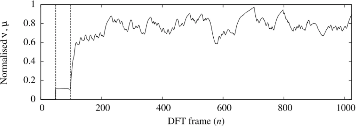
4.2 Evolution ofνn,µn. . . 33
4.3 Comparison between original and equalised DFTs. . . 33
4.4 Synchronisation progress. . . 33
4.5 Error pattern for off-coast tests. . . 33
List of Tables
4.1 FPGA implementation figures. . . 29
4.2 Parameters used for experimental tests. . . 30
Abbreviations
AUV Autonomous Underwater Vehicle ROV Remotely Operated Vehicle FSK Frequency-Shift Keying MFSK M-ary FSK CPFSK Continuous-Phase FSK PSK Phase-Shift Keying MPSK M-ary PSK DPSK Differential PSK
QAM Quadrature Amplitude Modulation DFE Decision Feedback Equaliser PLL Phase-Locked Loop
MIMO Multiple-Input Multiple-Output SISO Single-Input Single-Output
OFDM Orthogonal Frequency Division Multiplexing SNR Signal-to-Noise Ratio
ISI Inter-Symbolic Interference BER Bit-Error Rate
MLSE Maximum Likelihood Sequence Estimation RLS Recursive Least-Squares
LMS Least Mean Squares FEC Forward Error Correction DFT Discrete Fourier Transform FFT Fast Fourier Transform IFFT Inverse FFT
FIR Finite Impulse Response SS Spread Spectrum
FHSS Frequency-Hopping Spread Spectrum DSSS Direct-Sequence Spread Spectrum FDMA Frequency-Division Multiple Access FPGA Field-Programmable Gate Array HDL Hardware Description Language VGA Variable-Gain Amplifier
ADC Analog-to-Digital Converter DAC Digital-to-Analog Converter DDS Direct Digital Synthesiser SFDR Spurious-Free Dynamic Range
Chapter 1
Introduction
Sound has dominated underwater communication in the animal kingdom for millions of years. No other medium has the same ability to convey information at the large distances required, a situation comparable to that of electromagnetic waves over the air. Unfortunately, the harsh characteristics of the channel made its use for fast, reliable, and cheap communication lag behind the development of modern digital techniques, usually designed for use in more forgiving applications.
Since the 1970s, the evolution of digital electronics, as well as an improved understanding of the physical properties of the underwater channel and the associated design trade-offs, have propelled the development of efficient systems for both academic and practical use. The im-provement of incoherent receivers, with the emergence of capable DSPs, has led to low-rate but low-power and high-reliability systems. At the same time, the development of powerful coherent receiver algorithms in the 1990s, as well as the recent forays into spatial diversity and multi-carrier communications, make further improvements expectable. Advanced modulation schemes and equalisation algorithms, made possible by the availability of cheap processing power, brought underwater communications closer to their radio counterparts, and have fostered research into underwater networks for commercial and scientific applications.
However, most if not all of these systems have been developed with very specific use cases in mind: high rates in deep water, usually with simpler implementations; low rates but very low BER in control applications or shallow water; stealth communication for military usage; or high-powered coherent implementations for moderate rates in shallow water. Furthermore, few of them allow any substantial changes to their operation or support extensions to their functionality, con-sisting of monolithic implementations with fixed sets of parameters. The high cost of these sys-tems, as well as the added complexity, also precludes the use of a different unit for each operation scenario.
In several applications, it is essential for the system designer to have an easy way to experiment with different techniques and parameters under real conditions, in order to determine which are better suited to the task at hand. Even for the rather well studied incoherent receivers, according to
2 Introduction applications include AUVs moving between environments during their mission, untethered ROVs switching between video and telemetry feeds, stationary buoys operating in low power mode with occasional high-speed data bursts, or vehicles avoiding localised noise sources. In all of these cases, the design of the system will be simplified if the modem allows the necessary adjustments to be made in real time, without operator intervention.
In this dissertation, we set out to develop an underwater acoustic modem to serve as a flex-ible, configurable, and extensible communication platform, while taking advantage of existing equipment for underwater acoustics. To this end, the modem should:
1. permit experimentation with different modulations and diversity schemes; 2. allow the designer to analyse system performance both online and offline; 3. be parametrisable both online and offline;
4. allow configurable power consumption/performance trade-offs; 5. interface with available acoustic transducers.
This report begins by presenting existing work on the field, organised by area and chronolog-ically (Ch.2). The platform that was developed is described in Ch. 3, followed by experimental results obtained under real-world deployment conditions (Ch. 4). Finally, we conclude by sum-marising the contributions of this work and future work to be done (Ch.5).
Chapter 2
State of the art
2.1 Historical overview
As with most telecommunication technologies, the initial development of underwater communi-cations was largely driven by interest in commercial applicommuni-cations and military scenarios. In partic-ular, the increased use of underwater vehicles in the oil and gas industry during the 1970s created the need for untethered operation with a wireless command and control downlink [2]. During this decade, researchers identified the key limitations of the underwater acoustic channel and began using robust, incoherent modulation schemes, mainly MFSK [2,3]. While the throughput of these systems was very low, it was enough to transmit telemetry and control data.
It is interesting to note that as early as 1971 there was already a detailed conceptual under-standing of ocean multipath in acoustic communication, with work by Williams and Battestin [4] demonstrating completely analog multipath compensation, using Doppler invariant FM sweeps, by exploiting temporal coherence for channel estimation. The principles used in their work are largely the same that future developments were based on.
The 1980s brought the need for increased channel throughput, beyond what incoherent systems were capable of in the constrained bandwidth available. Video transmission, in particular, quickly pushed the requirements for underwater communication ahead of what was possible with early modems. In order to mitigate the problem, researchers began exploring the possibility of using coherent modulations, such as PSK, in vertical links. These are fairly benign in deep water, without the severe reverberation found in horizontal links, and as such research at the time focused on Doppler correction and changes in carrier phase with respect to range [5,6].
The advances in coherent systems were thought to be largely limied to vertical links, since the properties of horizontal links (particularly, dispersive multipath and time variability) seemed to make equalisation and phase tracking nearly impossible [7]. However, in the 1990s, Stojanovic et al. [8,9] demonstrated that coherent communication in the horizontal channel was feasible, using a powerful receiver structure combining an adaptive DFE with a second-order PLL for
phase-4 State of the art Later research has usually focused on one of two areas: decreasing receiver complexity, or increasing system performance as measured by the range-rate product [1]. These efforts have led to the use of spatial diversity (MIMO) techniques, as well as multi-carrier modulations (mainly OFDM) [10,11] and more computationally efficient equalisers and trackers [12,13].
A related issue that has been gaining weight is the evolution from point-to-point links to mesh networks. While this problem is outside of our scope, the interested reader may consult recent reviews on the subject for more information [14,15].
2.2 Channel modelling
1The underwater acoustic channel presents a number of properties that distinguish it from more traditional communication channels. In fact, in the words of a researcher in the field, they “are generally recognized as one of the most difficult communication media in use today” [16]. An understanding of the channel physics, and in particular its spatial and temporal coherence, is es-sential to the design of effective communication systems. While these properties are broadly the same across different channel types, in practice many of them take on different levels of impor-tance depending on whether the system is deployed in a deep or shallow channel, a calm or surf zone, or in a vertical or horizontal configuration.
Unfortunately for system designers, good statistical models for simulation are currently lack-ing, and even the statistical characterisation of the channel is up for debate. As such, the conclu-sions gleaned from a first-principles study should be used as a qualitative guideline, rather than a quantitative framework. A good review of channel models up to 2001 may be found in [19], while a more recent paper [20] summarises later advances.
The characteristics of the channel are mainly influenced by three factors: frequency-dependent path loss, time-varying multipath, and low propagation speed. These, combined with the specific circumstances of the communication system (such as transmitter-receiver motion), produce sig-nificant ISI and fading that must be taken into account by the receiver, while the presence of noise also cannot be discarded. These properties will be examined in the remainder of this section.
It is worth noting that some of these issues (notably, fading and multipath) are practically absent in short-range, high-frequency systems [21]. These, despite suffering from stronger atten-uation, may be well suited to high-throughput underwater networks where nodes are clustered together. Recent research in this area has sought to evaluate the feasibility of this technique [22, 23, 24], underlining the importance of an understanding of channel models for the practi-cal design of communication systems.
2.2.1 Propagation speed
The speed of sound in water (and, generally, in any medium) is several orders of magnitude lower than that of electromagnetic waves in air, originating different concerns. At any given point, the 1This discussion follows [16], abridging the mathematical treatment. For a more in-depth treatment of the physics of the underwater acoustic channel, see [17,18].
2.2 Channel modelling 5 1500 1540 1580 1460 Sound Speed (m/s) 0 1000 2000 3000 4000 Depth (m) Surface duct profile Mixed layer Main thermocline Deep sound channel axis
Deep isothermal layer Polar
region profile
Figure 2.1: Generic sound-speed profile. [18, p. 4]
propagation speed increases with both the local pressure and density of the medium. In a water body, these depend essentially on depth (pressure), and temperature and salinity (density). Since salinity is generally constant (except at locations like river mouths), its effect can be ignored in the speed variation. A detailed discussion of these effects is may be found in [17, 18], but it is important to understand the general variation profile of the propagation speed, represented in Fig.2.1.2
The most relevant characteristics of the profile are the slightly increasing speed in the initial mixed layer of the ocean, where temperature is approximately constant; the thermocline, a region of rapid decrease of temperature with depth, where the speed of sound tracks the temperature variation; and the deep isothermal layer, where temperature stabilises and pressure dominates [18]. This variation affects system design mainly due to multipath, as will be explored later in this section, and should be considered depending on the deployment scenario. In any case, a rough
6 State of the art
2.2.2 Attenuation and noise
The attenuation of sound underwater is mainly due to the transformation of acoustic energy into heat.3 In addition, the signal also suffers from spreading loss, due to the unfocused nature of sound emission. These two effects compound in the overall path loss, an increasing function of both distance and frequency. The profile of the frequency-dependent attenuation, modelled by an attenuation coefficient (in dB/km), is well known (see, for instance, [18, Fig. 1.20]), while spreading loss is modelled by a power law as a function of distance to emitter.
Besides attenuation, the total SNR also depends on the noise level of the medium. The ambient noise in the acoustic channel is usually characterised as Gaussian, but not white since its power spectral density decays at around 18 dB/decade. In most locations there is also a site noise com-ponent, which originates in local circumstances (most infamously by snapping shrimp producing cavitation bubbles with their claws [25]).
The product of these effects—frequency-dependent attenuation and ambient noise—is a vary-ing SNR over the signal bandwidth, but also over the transmission distance. In fact, for any given distance there is a centre frequency which maximises SNR (see [16, Fig. 1]), so that the available transmission bandwidth is also a function of distance. Empirically, we observe two important lim-itations: not only is the bandwidth severely limited (around 1 kHz at 100 km), but it is also on the order of the carrier frequency, which invalidates the usual narrowband assumption and exacerbates Doppler spread.
2.2.3 Time-varying multipath
The variation of the speed of sound with depth, along with the geometrical boundaries of the ocean (the surface above and the seafloor below), create pronounced multipath in acoustic transmission. This has important consequences for the temporal coherence of the channel and, therefore, for the design of the receiver. It is easiest to explain these effects in the context of ray theory [17], an approach identical to that of geometrical optics, even though it is only valid for high-frequency signals, as it ignores scattering and diffraction effects.
Multipath arises due to both refraction and reflection of sound. Reflections occur on the waveg-uide boundaries, and they are only specular under very particular conditions. Refraction happens on account of the varying speed of sound, and causes the arrival of a theoretically unlimited num-ber of rays even from a point source. The combined arrivals from the two effects make the channel reverberant and dispersive, and lead to a finite multipath spread on the order of tens of millisec-onds, the delay of the longest significant path.4
In practice, the impulse response of the channel almost always appears as a sparse sequence of discrete arrivals,5and so only a small number of paths are relevant. This is important in the design 3Scattering due to inhomogeneities in the water also plays a role, but it is sufficiently small in clear ocean water that we may ignore it.
4While every path acts naturally as a low-pass filter, and therefore introduces its own delay spread, for frequencies well below the channel cut-off this is not a significant effect. As high-rate systems push carrier frequencies upwards, however, designers may need to take it into account.
2.2 Channel modelling 7 of time-domain equalisers to mitigate ISI, since it heavily reduces the number of taps necessary. Also relevant, as always, is the type of channel under consideration: shallow water links suffer from harsher multipath due to the proximity of the reflecting surfaces and the larger variation of the propagation speed, while deep water vertical links are generally free from these effects.
To compound the problem, the characteristics of the arrivals are not constant, but instead vary significantly in time. Surface waves are the most important cause of this variation: by constantly moving the reflection point at the surface they change the path length, and therefore modulate the phase at the receiver. Other problems caused by surface waves are scattering and Doppler spreading (which will be examined shortly). The way these variations occur is very difficult to model statistically and also depends on the usage scenario.
The combination of the different echoes at the receiver introduces two unwanted effects: ISI, where the delayed arrivals from previous symbols affect the current waveform, and frequency-selective fading, where the randomly varying phase and amplitude of the echoes cause large varia-tions of the received signal strength at a given point in time as a function of frequency. Techniques to combat these problems have been well known for decades (for instance the Rake receiver [27]), but since they usually rely on either increased transmission bandwidth or powerful algorithms at the receiver, their use for high data rates in the field was delayed until the 1990s.
2.2.4 Doppler effect
The final channel property that bears discussing is the frequency shift and spread from Doppler effect, caused by relative transmitter-receiver motion. The magnitude of this effect is determined by the ratio a = v/c of relative velocity to propagation speed. While in radio communication channels the Doppler effect is only relevant for transmitters or receivers moving at high speed (such as Low Earth Orbit satellites or jet aircraft), the low speed of sound in water means that even platforms just drifting with the current can be affected. An added difficulty of underwater channels is the existence of Doppler effect from time-varying multipath, as discussed previously, since reflections from surface waves behave as additional emitters with their own independent velocities [26, p. 52]. Another undesirable coupling between the two effects occurs when the Doppler spread on each path differs.
The two effects, shift and spread, while physically related, are mathematically and conceptu-ally distinct. Doppler shift moves the signal spectrum to a different centre frequency by an offset of a fc (where fc is the carrier frequency). Doppler spread, on the other hand, changes the distri-bution of the spectrum, spreading or compressing it by a factor (1 + a). In single-carrier systems,
8 State of the art
2.3 Receiver topologies
From the analysis of the channel properties we can draw some general conclusions as to the design principles of underwater acoustic receivers:
1. Phase-coherent receivers will be difficult to implement in the highly reverberant and disper-sive shallow-water horizontal channel.
2. Incoherent receivers will maintain low BER in most applications, including those where coherent receivers have difficulty, at the cost of low spectral efficiency (and therefore low throughput).
3. Deep-water vertical links will be relatively clean of multipath, providing a good testbed for Doppler tracking algorithms and an easy environment for the implementation of high-throughput coherent receivers.
4. General-purpose receivers will be inefficient with respect to one or more figures of merit (BER, throughput, distance), since they must be designed with the worst-case channel in mind.
5. Because the channel will be, in general, far from clean, FEC codes are essential to guarantee acceptable BER levels.
These conclusions are upheld under real conditions, and should guide the choice of implemen-tation in any actual scenario. It is important to understand the diversity of strategies available to implement the receiver, and why some of the simplest methods are still widely used commercially. We will examine these various designs in this section, from the simplest FSK receivers to the latest MIMO-OFDM techniques.6
2.3.1 Incoherent receivers
Because of the difficulties exposed above to the implementation of phase-coherent receivers, early systems were based on incoherent modulations like FSK. FSK uses a set of pure frequency tones to represent the signal. Incoherent receivers for FSK typically employ a bank of correlators, or matched or bandpass filters, followed by envelope detectors, with local copies of the carriers un-synchronised with the source. The simplicity of this implementation, as well as its robustness in the face of phase and amplitude variation, made FSK a natural choice, since the channel is largely linear and the frequency content of the signal remains mostly within its original band. Multipath mitigation can be achieved using guard times between symbols [2] or tone reuse, to allow echoes to expire and eliminate ISI.
While the classic topologies above rely on the assumption of a linear channel, this is not strictly true under the presence of meaningful Doppler shift.7 In fact, under these conditions some form 6The oldest, analog techniques used in submarines will not be explored here, but it is historically relevant to recog-nise their existence and importance to the initial development of the field.
7While Doppler spread also introduces nonlinearity, it is not of as much concern for FSK systems, which only perform tone detection.
2.3 Receiver topologies 9 of Doppler compensation is required, or BER levels may become too high. One such method was implemented in DATS [29], where the transmitter emits a 60 kHz pilot tone which the receiver uses to correct for Doppler shift by bandpass filtering and PLL tracking. More recent systems [30] employ more sophisticated receiver-side processing, but the basic idea remains the same.
Incoherent systems for underwater communication have been researched since the early 1970s, but there have been no fundamental improvements since the introduction of diversity techniques (Sec.2.3.3). Instead, the evolution of computing power and hardware has led to the use of larger symbol constellations and higher rates. The simple implementation characteristics of incoherent FSK on both transmitter and receiver, together with its reliability under harsh channel conditions, promoted its continued use in offshore equipment, control downlinks for AUVs, and telemetry uplinks for oceanographic sensors [30], applications where data rates are not significant compared to the power consumption, processing power, and reliability requirements. Recent research has focused on the practical implementation details of FSK, from interoperability [31] to chip area [32] and the applicability to underwater sensor networks [33].
2.3.2 Coherent receivers
Despite their excellent BER and low implementation complexity, incoherent systems are limited to a spectral efficiency of 0,5 bps/Hz,8which strongly conditions their usefulness in modern high-throughput conditions (such as video uplinks from AUVs).
Coherent systems use both the phase and frequency of the transmitted signal to convey in-formation. They can achieve much higher R/W than incoherent systems, but they are more sus-ceptible to ISI. Because the phase reference is, by definition, placed at the transmitter, the most important implementation problems of coherent receivers are tracking the carrier phase and mak-ing correct symbol decisions in the face of phase noise.
The push for ever-increasing bit rates in the horizontal channel, along with the rapid growth of cheap processing power, led to the development of efficient and robust equalisation algorithms in the 1990s. The seminal work applying coherent modulation to the horizontal channel was done by Stojanovic et al. [8, 9], who derived a theoretically optimal, spatially-diverse receiver using MLSE. However, since the multipath delay is very long compared to the symbol period, with ISI spanning tens of symbols, MLSE is computationally prohibitive. An alternative approach is then proposed, where a suboptimal receiver is derived that replaces MLSE by joint carrier synchroni-sation and fractionally spaced DFE, greatly reducing the computational effort. The parameters of the receiver are adaptively adjusted using RLS and a second-order PLL, to handle phase tracking in the face of significant Doppler shift and spread.
Since its inception, this canonical structure has been modified and tested with a wide variety of equaliser methods and under various channel conditions. A summary of this work may be found in
10 State of the art have been identified for a long time, and many are described in [36]. Typical choices include: linear or non-linear (feedback) filtering; RLS or LMS for coefficient update; carrier tracking by PLL or equalisation filter; and blind or decision-directed equalisation. The use of DFEs also tends to amplify decision errors, and so a number of FEC codes have been used to compensate this. Notable improvements to the basic structure include the use of sparse equalisers (including partial response equalisers [37]), taking advantage of the discrete nature of the multipath to reduce com-putational complexity [38]; joint channel estimation, equalisation, and symbol decoding, using Turbo-like structures [39]; and diversity techniques, as described in Sec.2.3.3.
Complex time-domain equalisers are required with single-carrier modulations because the non-ideal channel response, with large time spread, introduces significant ISI. One way to reduce the receiver-side complexity is to apply multi-carrier modulation, dividing the available channel bandwidth into a number of sub-channels, each with approximately flat response [40]. A partic-ularly attractive form of multi-carrier modulation is OFDM, which uses orthogonal sub-carriers. OFDM can be implemented with a simple FFT/IFFT pair split between transmitter and receiver. The equalisation of OFDM signals can be performed entirely in the frequency domain, using a single tap with the estimated value of the corresponding bin in the channel frequency response. The first experimental results for underwater OFDM [41] revealed performance figures superior to SISO systems, even without optimisation. Since this early work, several other researchers have made improvements to the basic method, often adapting techniques from radio wireless commu-nication to the underwater channel [10,42,43,44].
Because OFDM relies on the orthogonality of its sub-carriers, Doppler shift can dramatically increase inter-carrier interference, to the detriment of system performance. This is especially so for the underwater channel, where Doppler shifts are large relative to the sub-carrier bandwidth. As such, there has been some focus on the implementation of accurate and efficient Doppler com-pensation methods for OFDM [45], a task made more difficult by the non-uniform nature of the effect.
Despite these advances, there are simpler “almost”-coherent systems in use, designed for the clear vertical channel, which achieve similar performance as coherent systems with much less complexity, at the cost of a slight increase in BER. These systems use DPSK [34, Sec. 5-2-8] to encode the data, using the phase of the previous symbol as a reference for the current one. The receiver structure for DPSK is of comparable simplicity to that of FSK, using quadrature matched filters followed by a phase comparator to make the symbol decision. For large SNR, the performance of binary DPSK is only slightly worse than that of binary PSK, making it an attractive choice for vertical channel communication.9 An early DPSK vertical telemetry system with good performance was described in [5].
9The performance of DPSK relative to PSK worsens as the number of symbols grows, tending towards a difference of 3 dB in SNR/bit for the same BER.
2.3 Receiver topologies 11
2.3.3 Diversity
Diversity is used in fading multipath channels to reduce error rates, by supplying the receiver with multiple copies of the original information transmitted over uncorrelated fading channels. This assumes that errors occur when the signal is strongly attenuated by fading in one channel, but not in another, uncorrelated one. Diversity complements traditional methods of handling noise, since the statistical characterisations of fading and noise differ significantly.10
The use of diversity is normally classified as temporal, frequency, or spatial. Whichever the specific method used, the key design requirement is that the separation between replicas exceeds the channel coherence, so that the different paths are resolved and the fading in each one is uncorre-lated. Basic diversity techniques include transmission on several different carriers with separation greater than the coherence bandwidth (frequency diversity), transmission on different time slots separated by more than the coherence time (time diversity), and transmission by different anten-nas with enough separation to cause discernibly different propagation delays on all paths (spatial diversity). Early examples of frequency diversity used in this manner may be found in [2,3].
There are also more sophisticated diversity methods available. Frequency hopping is a frequent choice for incoherent systems [35], due to its natural fit to FSK communication. Examples can be found as early as 1972 [46]. Frequency hopping, and spread spectrum (SS) techniques in general, provide implicit diversity by making the bandwidth of the transmitted signal much larger than the coherence bandwidth of the channel, which allows the receiver to resolve the individual multipath components.11 Coherent systems can also take advantage of implicit frequency diversity by using DSSS, which is better suited to PSK [47]. All of these wideband signals can be processed optimally by a Rake receiver [27].
If we look at the above diversity methods as coding techniques, they appear as repetition codes, whereby information is simply repeated over different channels to improve error rates. From this point of view, it becomes natural to attempt the use of better coding methods to improve performance. This is the idea behind coded modulation, introduced to underwater communications by Proakis in 1991 [48] using Hadamard-coded FSK. This system was commercially implemented, with good results, using 128 tones [30].
This coding method, similarly to SS techniques, expands the spectrum of the original signal to achieve frequency diversity. For the bandwidth-constrained underwater channel this is an un-desirable trade-off. Ideally, we would have a coded modulation capable of maintaining the signal bandwidth at the cost of some additional complexity. One such method, trellis-coded modulation, was introduced by Ungerboeck in 1982 [49], and it relies on an increase of the size of the sig-nalling constellation to make up for the coding redundancy. Its use in underwater communication has not been widespread, but examples can be found in [50,51].
12 State of the art that they don’t waste bandwidth or throughput on redundant information, instead making use of the available spatial bandwidth. Additionally, they are well suited to the use of trellis codes, as demonstrated in [51]. The initial application of MIMO techniques to underwater communication was done in 2004 [52], with good experimental performance. Yang [53] presents theoretical re-sults on the processing gain obtained in this and related ways. Further work demonstrating good system qualities includes [10,11,44].
2.4 Existing systems
A number of acoustic modems have been implemented since the beginning of digital underwa-ter communications, both for research purposes and commercial applications. We list the most relevant of these here for reference.
(A word of caution is important: the performance figures listed are supplied by the manufac-turers or research groups for optimum working conditions. In practice, and due to the nature of the environment, they are often not achievable by a large margin, and the lack of a testing standard makes direct comparisons meaningless [35].)
2.4.1 Commercial
Commercial modems are available mostly for telemetry, command and control, and positioning. Teledyne Benthos supplies the ATM-900 series, with modems rated for different depths capable of both shallow and deep water operation. For instance, the ATM-916 [54] is rated to 500 m with range up to 6 km. It operates in three frequency bands (9-14 kHz, 16-21 kHz, and 22-27 kHz), and reaches baud rates of 15360 bps with BER 10−7 under high SNR, using MFSK and PSK modulations.
Evologics markets the S2C R series, capable of full-duplex communication using frequency spreading. The S2CR 18/34 [55] is designed for medium-range, horizontal communication in shallow water. It is capable of 13,9 kbps up to 3500 m, using the 18-34 kHz band.
Develogic produces the HAM.NODE and HAM.BASE systems. HAM.NODE [56] uses either OFDM-DPSK or FSK with Doppler compensation up to ±12 m/s. It uses three frequency bands (8-13 kHz, 11-20 kHz, and 17-29 kHz) for a data rate of over 7000 bps in a 1950 m vertical channel. L-3 ELAC Nautik’s offer includes the UT 3000 MASQ [57], which uses frequencies in the 7500-19000 Hz range to achieve bit rates up to 1000 bps, with Doppler tolerance up to ±23 m/s.
Aquatec sells the AQUAmodem 1000 [58], operating in the 7,5-12 kHz band with FSK or DPSK and spread spectrum, for data rates up to 2 kbps.
Finally, LinkQuest [59] boasts proprietary spread spectrum technology with multipath com-pensation to achieve data rates up to 38400 bps with BER 10−9.
2.4 Existing systems 13
2.4.2 Research
A number of research modems have also been developed and published. The most well-known of these is the WHOI Micromodem, now with two published versions [31,60]. The second version is capable of using FH-FSK and PSK modulations in both shallow and deep water, supporting MIMO techniques. It is capable of up to 5000 bps, and it is designed to have low footprint and low power consumption.
Benson et al. [61,33] have explored FPGA-based modems, using FSK modulation and custom transducers for a system focused on short-range communication within networks. Similar work with FSK FPGA-based modems has been done by Li et al. [32] exploring the design space of FPGA implementations with respect to BER, power consumption, and implementation area.
Finally, the rModem [62,63] has also taken a reconfigurable approach, but with an emphasis on PC-based Simulink software to implement physical, data link, and network layers.
Chapter 3
System description
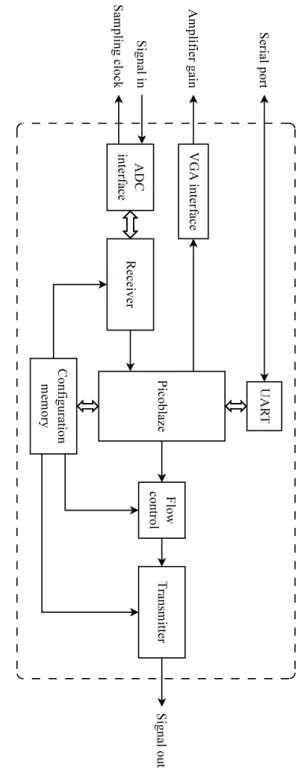
In order to meet the requirements established for the system, the digital section of the modem was designed according to the architecture in Fig.3.1. The user interface uses a serial port for control and monitoring. The central control tasks are performed by a soft core, the Xilinx Picoblaze, which besides running the state machine for the serial protocol also handles data reception and transmis-sion. The real time configurable (streaming) parameters are stored in a configuration memory, written by the Picoblaze and read by the other main blocks. The analog front-end, consisting of a VGA and an ADC, is configured by both the core and the receiver, while the waveform for transmission is output using a sigma-delta modulator.
In this chapter, we will describe each of these sections in detail. We begin with a discussion of the general design choices made in the project, as well as the implementation of modem-wide functions and the process followed throughout. We then present the details of both main blocks, the transmitter and the receiver, and the trade-offs made in their design.
3.1 General design choices
3.1.1 Hardware
Given the nature of the computation in a digital modem, implementations traditionally use soft-ware running on DSPs, which provide efficient primitives for signal processing, or ASICs, custom-designed for the application. However, both of these approaches have significant drawbacks in realising the goals stated in Ch.1:
• DSPs potentially have the lowest development time, but serial execution and fixed resources limit their throughput. Existing research [64, 61] also suggests that DSPs underperform FPGAs in power efficiency when the design is highly parallelisable, as is the case here. • ASICs, despite being the most area- and power-efficient option, have huge development and
16 System description Figure 3.1: General system architecture.
3.1 General design choices 17 In order to maximise the flexibility of the platform while simultaneously maintaining high performance, we chose to implement the system on an FPGA. The reconfigurability afforded by these devices also simplifies the extension to higher numbers of channels or complementary tasks. For this work, we used an OHO-Elektronik GODIL board [65], a development board based on a Xilinx Spartan-3E XC3S500E FPGA [66] which also contains an SPI-programmable flash memory and a 49,152 MHz crystal oscillator, used to generate the internal 98,304 MHz clock. The XC3S500E contains around 4600 slices, as well as 20 Block RAMs (BRAMs) of 18 kbit each and 20 dedicated 18 × 18 bit multipliers. The development board was mounted on a custom analog front-end board developed for a previous project [67], which performs signal conditioning and A/D conversion. The signal processing chain will be described in depth in Sec.3.3.
3.1.2 Channel coding
As the error rates in the underwater acoustic channel are generally high, it is essential that the transmitted data is encoded prior to transmission, so that a large fraction of the errors may be de-tected and corrected at the receiver. While FEC coding and decoding were planned to be included, and the system architecture was designed accordingly, the time frame for the project did not allow a hardware implementation. A simple way to provide this feature in the short term, at the cost of some processing overhead, is to add it to the control software.
3.1.3 Modulation
Since the underwater acoustic channel is bandwidth-limited, the theoretically optimum choice of modulation would be PSK or QAM. As we have seen in Ch. 2, however, the demodulators for these receivers are much more complex than those for noncoherent modulations. Furthermore, even though the channel is bandwidth-limited, the transmitters are often power constrained. Given these considerations, we chose to implement an FSK modem, which allows a smaller and more power-efficient implementation, at the cost of reduced throughput. FSK modems are also more robust in a wider variety of scenarios than phase-coherent modems, an important property since the envisioned use cases may require deployment under difficult conditions.
It is possible to improve upon basic FSK at little to no implementation cost by ensuring that the transmitted signal has continuous phase (CPFSK). The advantages of preserving the signal phase from symbol to symbol are reduced bandwidth (for appropriate parameters) and decreased sensitivity to timing errors [68], especially due to Doppler effect.
18 System description
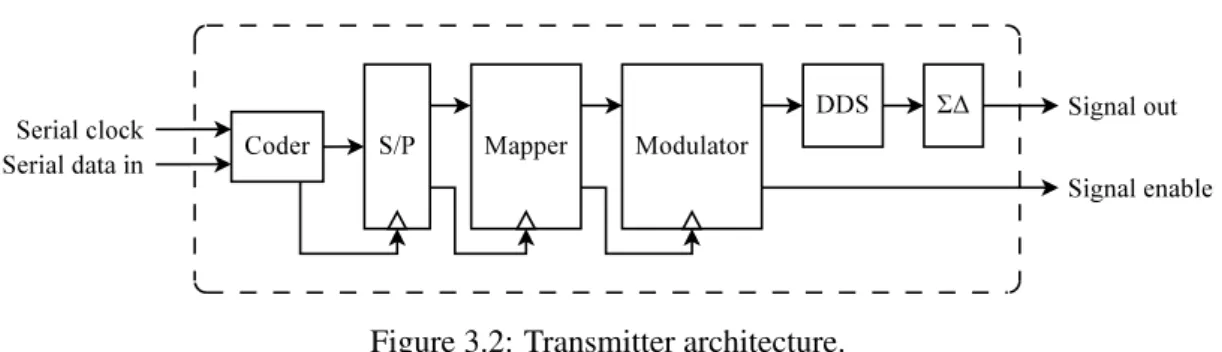
Figure 3.2: Transmitter architecture.
and this is the lower limit used here. Apart from having appropriate transducers readily avail-able, the advantage of using this band is the propagation distance/bandwidth trade-off [70], which matches the requirements for the system.
3.1.5 Control interface
The modem is controlled through an RS-232 serial link, making use of on-board level transla-tors. A custom protocol was developed to configure the modem and transmit and receive data, by addressing a set of configuration registers. The protocol is frame-based, using PPP-style byte stuffing [71], and it is parsed by a Picoblaze core [72] on the FPGA, which consumes very few re-sources and provides an efficient mechanism to implement complex state machines without strict timing requirements. Additionally, other functions, such as automatic gain control, may be mul-tiplexed onto the core with no increase in implementation size. On the PC side, the protocol was implemented by a command shell with additional scripting facilities.
3.1.6 Methodology
The nature of the project, containing elements of digital design, signal processing, and telecom-munications, implied a design and verification effort on two fronts:
• the processing chains, in particular for the receiver, were first implemented as Simulink models, to allow for fast experimentation and fine-tuning without the complexity of a (harder to verify) HDL description.
• the HDL implementation was verified through extensive functional simulation, with real data from tests and synthesised stimuli. Whenever possible, IP cores from the FPGA man-ufacturer were used in order to shorten development time and improve performance.
3.2 Transmitter
The transmitter is very compact, but designed for easy extension to techniques like frequency hopping or coded modulation. The architecture (Fig.3.2) uses serial input, since FEC coding may be convolutional or by blocks. A serial-to-parallel (S/P) block is included to take into account the general case.
3.3 Receiver 19
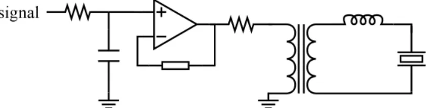
Figure 3.3: Transmitter output circuit.
3.2.1 Symbol mapping and modulation
After parallelisation, the coded words are mapped to symbols for modulation, using Gray code to minimise the error probability. The modulator is then responsible for converting the symbols into an FSK-modulated analog waveform. The mapping from symbols to frequencies is completely configurable in real time, opening up the possibility of using band allocation for multiple access to the channel (FDMA), or adapting to narrowband noise or interference.
To generate the analog waveform a DDS core is used [73], with 14-bit output, a 4096-entry look-up table, and a 20-bit internal accumulator for a frequency resolution of 93,75 Hz. The implementation uses phase dithering [74] for improved SFDR (84 dB, or 12 dB better than phase truncating). The small size of the DDS makes it feasible to add extra instances in order to support frequency diversity or multi-carrier modulations. The final advantage of using a DDS is that the phase of the output is always continuous unless a phase offset is purposefully introduced, making CPFSK generation trivial.
3.2.2 Signal output
The output circuit of the transmitter is represented in Fig. 3.3. Since the front-end board lacks a DAC, and to cut back on hardware costs, a sigma-delta modulator (Σ∆M) was implemented in front of the DDS, driving an I/O pin which is then low-pass filtered to produce the output waveform for the transducer driver. The driver uses a TDA2003 audio amplifier [75], capable of supplying 10 W continuously to the load, which consists of the primary winding of a transformer along with a series resistor to equalise the frequency response. The transducer is driven by the secondary winding, with a series inductor for impedance matching.
In addition, to provide the user with control over the transmission power, a gain configuration register can be used to reduce the amplitude of the transmitter output before it feeds theΣ∆M.
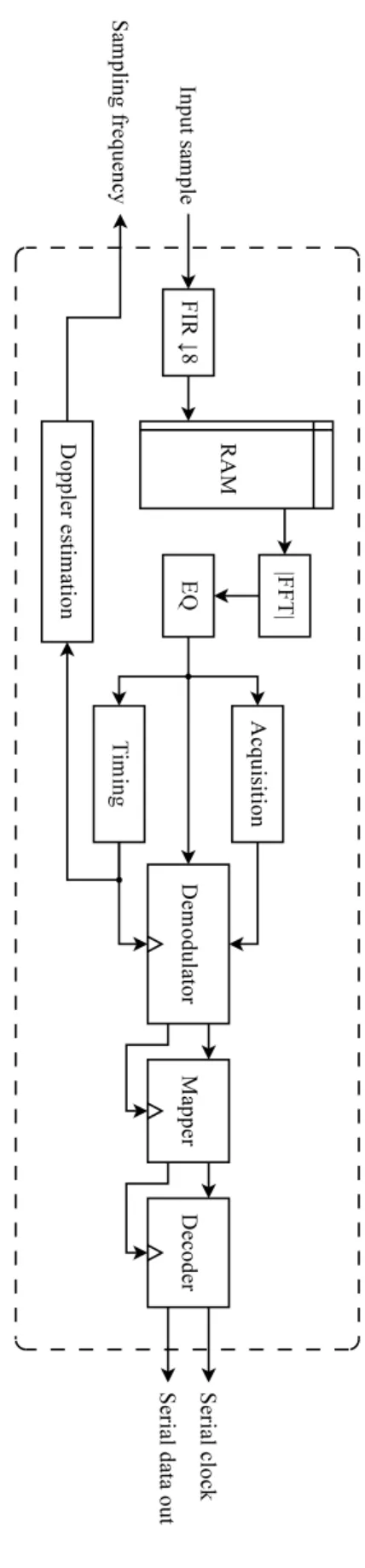
20 System description Figure 3.4: Recei ver architecture.
3.3 Receiver 21
(a) M = 2
(b) M > 2
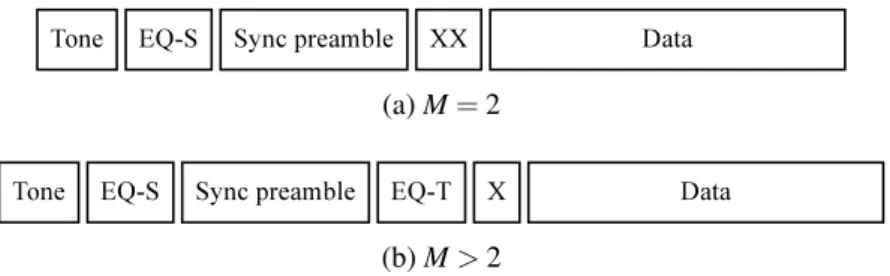
Figure 3.5: Frame sequences for constellations with M symbols.
• Flexibility: with an unchanged FFT core, it is possible to vary the number of symbols in real time, as well as acquire their frequencies without performing spectrum sweeps. • Extensibility: apart from its flexibility within the current architecture, using a DFT also
simplifies future extensions to include frequency diversity, particularly frequency hopping. • Resilience: while receivers using local oscillators need complex frequency tracking
algo-rithms, particularly to compensate Doppler effect, a simple symbol decision criterion can make a DFT-based receiver immune to frequency offsets and drift [76,77,78].
We have also found that all of the processing downstream from the DFT was simplified, and could be made to work with much smaller bus widths than would otherwise be possible. This is an important characteristic for FPGA implementations, which have limited routing resources available. Finally, because all of the sequential algorithms have pipelined implementations, no storage is used for the FFT result.
An important feature that was not implemented is automatic gain control. As it can be seen from Fig.3.4, this was not included directly in the receiver architecture, but rather was planned to be added to the code for the Picoblaze core (Fig.3.1). This would not use any additional physical resources, while keeping up with the comparatively relaxed timing requirements of the task.
3.3.1 Frame sequence
The communication between two modems is structured around frames, which begin with a header sequence of symbols designed to initialise the various receiver blocks (see also Fig.3.5, where X denotes a previously used symbol):
1. Acquisition tone: the symbol with lowest frequency1is sent for NAsymbol durations (tsym) for signal and frequency acquisition (Sec.3.3.4). The information from the tone is also used to equalise the response to that symbol (Sec.3.3.5).
22 System description the signal window only contains one frequency. After the starter, the equaliser begins for the synchronisation preamble.
3. Synchronisation preamble: this section consists of an alternating sequence of symbols (say 010101...), lasting for NStsym. The sequence is used to synchronise the DFT calculation to the symbol boundaries, by making use of the transitions to align the transform window (Sec.3.3.6).
4. Equalisation tail: if the signal constellation contains more than two symbols, the ones that were not yet used are sent after the preamble and used to complete the equaliser coefficients. The equaliser is disabled for the tail, to prevent the new symbols from being masked by the echoes of the preamble.
5. Data: if an equalisation tail exists, the data section is started by transmitting a single symbol from the ones used in the preamble; otherwise, it begins with any two repeated symbols. This frame sequence is controlled by a separate state machine (not shown in Fig.3.5), which enables and disables the receiver modules according to the current point in the sequence.
3.3.2 Signal conditioning and input
The signal input to the front-end board comes from an identical transducer to that used in the transmitter, or the same if half-duplex communication is used. It passes through a fixed-gain pre-amplifier, followed by a VGA and an anti-aliasing filter, which feed a 12-bit ADC capable of up to 1 Msps sampling rate. This configuration has an input band of 10 to 250 kHz, which allows the use of different transducers and frequency bands [67]. The actual sampling frequency chosen is 768 kHz, which exactly divides the clock frequency and avoids aliasing.
Once the signal is converted, a digital polyphase decimator FIR filter is used to filter out-of-band noise and lower the sampling rate to 96 kHz (decimation factor 8). The filter is implemented in the FPGA using a Xilinx IP core [79], with a passband of 19 to 29 kHz, 14-bit coefficients, and 31-bit output words (then truncated to 16 bits). Given the low frequencies involved, there is no downconversion of the input signal to zero. The filtered input samples are then stored for processing.
3.3.3 DFT calculation
The DFT on which the receiver is based is calculated by a 256-point FFT core [80] with a reduced radix-2 implementation, producing a 16-bit complex output using 16-bit coefficients. A fixed scaling schedule of 1/2 at the input of each stage is used to avoid overflow. A standard analysis of the quantisation noise at the output of an FFT [81, Sec. 9.7] shows that the output SNR for this configuration is around 60 dB.
Because the receiver is noncoherent, the phase information is discarded as noise and only the magnitude is used. To obtain the magnitude, and to avoid the use of costly functions like CORDIC, the method in [82, Sec. 10.2] is used: the maximum and minimum of the absolute values of the real and imaginary parts of the DFT are calculated, and the magnitude is then estimated as
3.3 Receiver 23 α ·max|·|+β ·min|·|, whereα and β are suitably chosen constants. By choosing α = 1 and β = 3/8 only four adders are used, with a peak error of −23 dB.
The number of samples used to calculate the FFT depends on the symbol rate. For rates above 375 baud (96 kHz/256), the input is zero-padded. Rather than always using a single transform per symbol, different amounts of overlap are used for the different parts of the frame sequence. For the initial acquisition, two DFTs per symbol are calculated, while for the synchronisation preamble the overlap depends on the maximum allowable timing error (Sec.3.3.6).
3.3.4 Frequency acquisition
Reception begins with the identification of a signal above the noise, and the DFT presents a natural way to detect and acquire the tones used in the frame header. The general strategy of our frequency acquisition algorithm is to estimate the noise floor to threshold the DFT magnitude, acquiring any tone that is steadily above this level. To determine the correct tone a voting system is used, where the candidates are the bins on each side of the initial peak and votes are attributed once per trans-form, going to the candidate that presents the maximum magnitude. If, after acquisition, the DFT drops below (another) threshold for too long, the acquisition lock is lost. In detail:
Parameters αa,αd∈ (0,1): time constants for noise floor and peak level estimates. βa,βd≥ 1: threshold multipliers for acquisition and de-acquisition. NI,NA,ND>0: number of DFT frames to process in each stage. Ns≥ 0: number of side bins to consider for acquisition.
Nv>0: minimum number of votes for acquisition.
Inputs Xn
k: the magnitude of the k-th bin of the n-th DFT frame. Outputs kt: the bin of the acquired tone.
Variables νn,µn: the noise floor and peak estimates, respectively. Initialisation For NIframes:
I.1. Update νn=αamaxk{Xn
k} + (1 − αa)νn−1(withν0=0). Acquisition For each frame:
A.1. If maxk{Xn
k} > βaνn:
A.1.1. Let kc=argmaxk{Xkn} and νc=νn.
A.1.2. For NA frames, count the number of frames (votes) for which the magnitude of each bin in the range [kc− Ns,kc+Ns]is maxi-mum and exceedsβaνc.
24 System description De-acquisition For each frame:
D.1. If maxk{Xkn} < µn/βd:
D.1.1. Count the consecutive frames for which the condition holds. D.1.2. If the count reaches ND, the algorithm restarts atI.1.
D.2. Else, update µn=αdmaxk{Xkn} + (1 − αd)µn−1.
The DFT frames are calculated using half a symbol of overlap, as suggested in [83], in order to keep the acquisition tone short while maintaining the correlation of consecutive frames as low as possible. While other implementations use the average power in each candidate bin [77], we have found that the additional computational overhead did not improve the results over the use of a voting system. The limitation to Nsbins on each side of the centre candidate, instead of the entire spectrum, is meant only to avoid the use of extra storage.
The estimates are updated using an exponential moving average (EMA), rather than e.g. a simple moving average (SMA). The main properties of the EMA that motivate its use here are its resource efficiency, requiring only storage for the previous estimate; the larger weight it gives to more recent observations, making the response faster; and the advantages it displays over the use of SMA, namely the lack of phase shift and inversions of the input, both of which could increase the rate of false positives in a noisy channel.
The biggest disadvantage of this algorithm is the need to adapt theαa,dandβa,d parameters to each scenario: multipath-heavy channels require largeαdand lowβddue to large coherence times, while on cleaner channels the (de-)acquisition may be accelerated by decreasingα and increasing β. Values that were found to produce good results are αa=1/4,αd=1/16, andβa=βd=2. The use of powers of two is intentional to avoid the use of multipliers, and it is sufficient to get good system response.
3.3.5 Equalisation
Since neither the transducer nor the channel frequency responses are flat, and because of the strong multipath present underwater, it is essential to equalise the received signal in order to maintain a low error rate. While an electrical model for the transducers is available, and it is possible to equalise for it at the transmitter, the most flexible option is to dynamically adapt the equaliser with measurements of the complete response from the channel and transducers.
To do this without adding considerable overhead to the frame or complex coefficient adaptation algorithms, like LMS or RLS, a band equaliser was implemented. The bands are centred on the DFT bins corresponding to each symbol, extending to each side for half the symbol frequency spacing. The equalisation coefficients are initialised in the frame header and updated with each new symbol.
All coefficients are powers of two, allowing a very efficient implementation based only on logical shifters. While the equalised response is not as flat as that produced from coefficients
3.3 Receiver 25 0 1 (a)λ = 0 0 1 (b)λ = 3/8 0 1 (c)λ = 4/8 0 1 (d)λ = 6/8 Figure 3.6: Effect of timing offset on DFT.
calculated by a full division, it is sufficient to keep it within a predetermined band around the target value. More concretely: for each bin k, given a target magnitude XT =2t and a maximum deviation of∆T =XT· 2−m(for some t,m ∈ N0), the corresponding coefficient Qkis calculated so that XT− ∆T ≤ QkXk ≤ XT+∆T. This corresponds to assuming that at least m most significant bits of the bin magnitude remain constant. The larger m is, as long as this assumption holds, the flatter the response, but the less tolerant the algorithm is to fading. In practice, values of m = 3 or 4 have been found to produce good results in all test scenarios.
3.3.6 Symbol timing synchronisation
A critical aspect of the receiver performance for a noncoherent system is the accuracy of the symbol timing synchronisation. The error probability increases markedly at even small levels of error (as measured by λ = ∆t/T, where ∆t is the absolute timing error), and the situation worsens with increasing constellation size. Since only the DFT magnitude is used, the most direct timing information present in the signal phase is lost, making synchronisation more difficult. Our
26 System description Because the preamble consists of alternating symbols, an offset DFT will contain spectral con-tent from two frequencies. This effect is illustrated in Fig.3.6, where the DFTs of a symbol pair are illustrated for four offsets, along with the window (in grey) for which they were calculated. The transition between frequencies is very noticeable, withλ = 4/8 being the case for which the most leakage occurs. It can be seen that the difference between the magnitudes of the two symbol bins presents a good metric from which to estimateλ. The idea behind the algorithm is to max-imise this difference in order to find the correct timing offset:
Parameters NO≥ 2: number of offsets to examine.
NS≥ 2: number of symbols on which to run the algorithm. Inputs k0,k1: DFT bins corresponding to the preamble symbols.
Xk: the magnitude of the k-th bin of the current DFT frame. Outputs noff: synchronised offset of DFT window.
Variables n: current symbol index. i: current offset.
µi
n: metric for offset i of symbol n.
Algorithm
1. For NSsymbols:
1.1. For NOoffsets, letµi
n=|Xk0− Xk1|.
1.2. Increment the vote count for offset argmaxi{µn}.i 2. noffis assigned the offset with the largest vote count.
The performance of the algorithm is inextricably linked to the equalisation performed up-stream. In practice we observe that, with high-Q transducers and no equalisation, the sign of the metric may be inverted—the current symbol is not the dominant DFT peak—due to multipath and skew the results heavily. This happens because one of the symbol frequencies may be much more attenuated than the other, so that the echo of the previous symbol dominates the DFT.
The number of offsets for which to calculate the DFT depends on the maximum timing error allowed. For CPFSK with noncoherent detection, it may be shown [68] that the loss of SNR for λ = 1/16 at a BER of 10−4 is under 0,1 dB, and so NO=8 is sufficient to produce good results even for 8-symbol constellations.
3.3.7 Doppler estimation
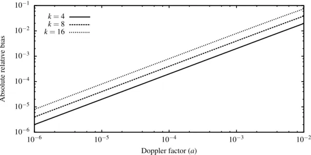
The information obtained from the symbol timing algorithm may be used to estimate the Doppler effect of the channel with enough precision to adjust the ADC sampling rate. While it would be more natural to use the DFT for this task, a frequency resolution of 375 Hz means that, for the shift to be noticeable even in the absence of noise (i.e. just over half a DFT bin), the relative speed between the transmitter and receiver would have to be over 10 m/s, which is not a realistic
3.3 Receiver 27 scenario for most underwater operations. On the other hand, even with speeds as low as 1,5 m/s (a = 10−3), the symbol timing estimate will be off by more than the synchronisation precision (1/16 of a symbol) after just 63 symbols (a−1/16)2, which will increase the error rate.
These numbers suggest a precise way to estimate a by reusing the resources already allocated to symbol synchronisation, which would otherwise be idle after the frame header. If the window offset votes are counted on every symbol transition, rather than just during the synchronisation preamble, a constant a will produce a constant increase or decrease of the estimated offset. In fact, if a sliding window of size NSis used to count the votes, the magnitude of the Doppler effect may be estimated as
ˆa = 1 NO(n2− n1),
where n1,n2 are the indices of the symbols when the first and second increase (or decrease) in offset occur. While not unbiased, the estimator has a small enough expected relative error that it may be used to adjust the ADC sampling rate. See AppendixAfor the full derivation of the estimator and its properties.
While this algorithm was not implemented, the modifications to the existing structure would be small, requiring only that the synchronisation module continue active after the frame header, use a sliding window for the votes, and take into account only symbol transitions.
3.3.8 Demodulation and word mapping
The centrepiece of the receiver is the demodulator, which is responsible for identifying the trans-mitted symbols in the equalised DFT. A number of symbol decision criteria for DFT-based re-ceivers have been proposed in the literature [84,76,77], with varying complexity and performance. Because we have assumed small Doppler shifts in the symbol frequencies, we implemented the common criterion of picking the symbol whose nominal frequency is closest to the maximum of the DFT.
The final step in the receiver chain is the mapping from Gray-coded words to binary, using a small look-up table. The result is the channel-coded word, or a corruption thereof, which would be corrected for by the FEC decoder.
Chapter 4
Results
Once the implementation of the system was finished, a number of experimental tests were per-formed to determine its performance and compare it with existing systems, as well as with our proposed objectives. We will now describe these tests and analyse their results in detail, in order to get a sense of how well the design trade-offs made work under real conditions.
4.1 FPGA implementation figures
The resource usage results for the FPGA implementation are shown in Table4.1. It can be seen that, although there were no low-level optimisation efforts, the design takes up only slightly over half the existing slices. A large number of multipliers and BRAMs remain available to extend the design or add a more capable soft core.
Resource Used/available %
Clock buffers 2/24 8
Digital clock managers 1/4 25
Multipliers 4/20 20
Block RAMs 7/20 35
Slices 2449/4656 52
Picoblaze instructions 192/1024 19
Timing slack 0,043 ns
Table 4.1: FPGA implementation figures.
4.2 Experimental setup
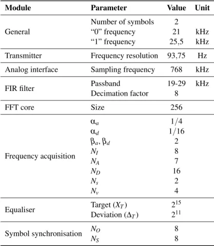
30 Results
Module Parameter Value Unit
General
Number of symbols 2
“0” frequency 21 kHz
“1” frequency 25,5 kHz Transmitter Frequency resolution 93,75 Hz Analog interface Sampling frequency 768 kHz FIR filter PassbandDecimation factor 19-298 kHz
FFT core Size 256 Frequency acquisition αa 1/4 αd 1/16 βa,βd 2 NI 8 NA 7 ND 16 Ns 2 Nv 4
Equaliser Target (XTDeviation (∆T) ) 221511 Symbol synchronisation NONS 88
Table 4.2: Parameters used for experimental tests.
ysed in this chapter (such as pool tests with very large coherence times). However, several of these, most importantly those marked as general, should be varied in order to obtain a more complete profile of the performance of the modem.
The decision to use symbol frequencies so far apart, instead of trying to minimise the occupied bandwidth, warrants some explanation. While such a large frequency separation reduces the error probability at the symbol decider, it strongly increases it at the synchronisation preamble (which is the crucial section of the reception process) due to the high-Q response of the transducers, which allows us to better exercise the equaliser. Since the decider is fairly standard, its performance was not as much of an unknown, and we chose instead to verify the joint behaviour of the equaliser and the synchronisation algorithm.
4.2.2 Setting
The first series of experiments was performed at the Leixões Marina. This is a more challenging setting than the open sea given the plethora of obstacles, like boat keels, contributing to the channel multipath. On the other hand, the achievable test distances are small compared to those used in most real scenarios.
4.3 Marina results 31 The second series of tests was performed off the coast of Leixões, in approximately 10 m depth, allowing larger distances. The transmitter was placed aboard the boat used for the tests, while the receiver was attached to a moored buoy. Because of this arrangement, with both nodes drifting, it is difficult to provide precise figures for distance and relative velocity.
4.2.3 Methodology
All tests used a stationary or drifting receiver and a mobile transmitter, with the transmitter being placed at different distances from the receiver. Along with the receiver board, a digitalHyd SR-1 hydrophone was used to record unprocessed audio at a small distance (~3 m) from the receiving transducer, with a sampling rate of 101,562 kHz. Due to implementation problems at the time of the experiments, all the results presented here were obtained from functional simulation of the HDL implementation, using the recorded audio as input (resampled to match the ADC frequency). Three types of test data were used, in order to better understand the error patterns of the receiver under different conditions: all equal symbols, alternating 00/FF bytes, and random data (Bernoulli process with 0,5 probability for each outcome). Only the results for random data, which are more representative of the true receiver performance, will be analysed.
Although several distances were used for testing, due to implementation problems only a few of them produced valid data. The results for these will be analysed below.
4.3 Marina results
The best results were, as expected, obtained at the shortest test distance (~5 m). Using a symbol rate of 750 baud, over a run of 2048 bits, 7 were wrongly detected, making for a bit error rate of 3,4 × 10⁻³. The 90% confidence interval for the BER is [1,6; 6,4]×10−3.
The observation of wrong bit decisions leads to the conclusion that these are caused over-whelmingly by multipath, rather than channel noise. In fact, as Fig.4.1shows, there is very little variance around the nominal symbol bins (56 and 68), indicating that when errors occur they are mostly due to interference.
200 400 600 800 1000 Occurrences
![Figure 2.1: Generic sound-speed profile. [18, p. 4]](https://thumb-eu.123doks.com/thumbv2/123dok_br/18881034.932512/27.892.237.701.140.660/figure-generic-sound-speed-profile-p.webp)