ABSTRACT: This paper applies the frequency response methodology to characterize and analyze the lying qualities of longitudinal and lateral axes of a rotary-wing aircraft, AS355-F2. Using the results, it is possible to check the suitability of the aircraft in accordance with ADS-33E-PRF standard, whose lying qualities speciications criteria are based on parameters in the frequency domain. The key steps addressed in the study involve getting, by means of light test data, the closed-loop dynamic responses including the design of the instrumentation and speciication of the sensors to be used in the light test campaign, the deinition of the appropriate maneuvers characteristics for excitation of the aircraft, the planning and execution of the light test to collect the data, and the proper data treatment, processing and analysis after the light. After treatment of the collected data, single input-single output spectral analysis is performed. The results permit the analysis of the lying qualities characteristics, anticipation of the demands to which the pilot will be subjected during closed-loop evaluations and check of compliance with the aforementioned standard, within the range of consistent excitation frequencies for light tests, setting the agility level of the test aircraft.
KEYWORDS: Flight characteristics, Helicopters, Flight tests, Frequency-domain analysis.
Management Process of a Frequency
Response Flight Test for Rotorcraft Flying
Qualities Evaluation
João Otávio Falcão Arantes Filho1, Donizeti de Andrade2
INTRODUCTION
he aircrat lying qualities, for both rotary and ixed-wing aircrat, determine the easiness and precision with which the pilot is able to perform the operational tasks that constitute the mission proposed for that air vehicle (Williams et al. 1995). Flying qualities evaluations aim to measure the pilot skill level required to operate the aircrat and are a method to verify the suitability of it for a given mission (Brasil 2003).
Flying qualities evaluations can be conducted in qualitative and quantitative ways. Qualitatively, they are assessed by testing in closed-loop form (pilot-in-the-loop), in which the pilot efectively acts on the light controls to fulill certain task.
here is a task requirement (desired or adequate performance to be reached), a pilot action in the light control system to meet this requirement, the reaction of the aircrat according to its aerodynamic characteristics and an efectively achieved response. he pilot observes the aircrat response, determines the error between the actual and desired response and, if in fact the error exists, he (she) performs an additional control input to reduce or eliminate it. In the end, he (she) considers all actions applied on light controls and the performance reached to determine the overall workload due to the compensation of the aircrat deiciencies (efort and attention required) added by that due to the properly execution of the task (Brasil 2003). hen he (she) employs the handling qualities rating (HQR) like the Cooper-Harper scale (Cooper and Harper Junior 1969). In addition, other factors inluence the inal rating given by the pilot, such as the interface with the cabin (displays, commands and controls), the environment (weather, visibility
1.Departamento de Ciência e Tecnologia Aeroespacial – Instituto de Pesquisas e Ensaios em Voo – Divisão de Ensaios em Voo – São José dos Campos/SP – Brazil. 2.Departamento de Ciência e Tecnologia Aeroespacial – Instituto Tecnológico de Aeronáutica – Departamento de Projetos – São José dos Campos/SP – Brazil.
Author for correspondence: João Otávio Falcão Arantes Filho | Departamento de Ciência e Tecnologia Aeroespacial – Instituto de Pesquisas e Ensaios em Voo –
Divisão de Ensaios em Voo | Praça Marechal Eduardo Gomes, 50 | CEP: 12.228-901 | São José dos Campos/SP – Brazil | Email: [email protected]
and turbulence), the requirements that deine the mission and the stress (Brasil 2003). Figure 1 represents the block diagram of a closed-loop evaluation.
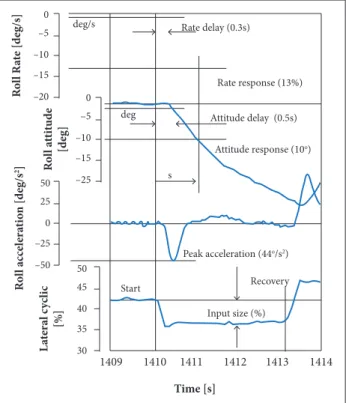
In the quantitative form, the characteristics of stability and control that directly afect the lying qualities are obtained. hese tests evaluate the characteristics linking the light controls to the aerodynamic response by means of the light control systems. hese tests are based on open-loop tests, carried with the pilot out of the control loop, in which the environment, the pilot or another device connected to the light control system perform a predetermined control input. hen, the aircrat response is observed and measured (United States Naval Test Pilot School 1995). Objectively, these tests are responsible for system identiication. Figure 2 illustrates the characteristic parameters of any rotary-wing aircrat response able to be obtained in an open-loop test, by a step control of lateral cyclic.
Aircrat system identiication is the methodology by which a mathematical description of the dynamic characteristics of an air vehicle can be extracted from the light data (Williams et al. 1995). It is a procedure that allows obtaining dynamic models from the aircrat response measured by light tests speciic control inputs. he inputs are applied to excite the dynamics of interest to which the model is employed, e.g. the one aiming at characterizing the light mechanics of a complete aircrat, or a speciic system, such as an actuator, engine or rotor of a rotary-wing aircrat. Typical applications of aircrat systems identiication are: simulation models; development and validation of flight control systems; assessment of the lying qualities characteristics and check of compliance with the lying qualities requirements (Tischler and Remple 2012).
In the aircraft system identification field, a study of its historical development is done by Hamel and Jategaonkar (1996). his study briely discusses from the estimation techniques used in the early 20th century to obtain light stability derivatives to current methods, which were drastically changed by the data processing capability of digital computers. Special attention in that study is given to the “quad-M”, four interrelated topics
that should be thoroughly investigated and that are key to the success of a system identiication: (a) maneuvers (control inputs) able to excite the dynamic modes; (b) selection of instrumentation system and iltering features for obtaining accurate measurements; (c) deinition of the structure of the mathematical model (which depends on the type of vehicle to be investigated); and (d) quality of data analysis, based on the selection of the most appropriate method of identiication.
he traditional techniques for lying qualities assessment involve, primarily, the time-domain analysis of the responses to certain control inputs, like steps, impulses, or doublets. he study focuses on the parameters such as rise time, time constant, time to double (or to decay by half) the amplitude, natural damped frequency and damping ratio. With the advent of augmented light control systems in rotorcrat — with large bandwidth or
Figure 1. System pilot-aircraft (Cooper and Harper Junior 1969).
Stress Aural cues
Visual cues Motion cues Pilot
Task Control force Control displacement
Feel Controlsurface
servos Control
laws
Aircraft Response External disturbances turbulence; crosswind Figure 2. Characteristic parameters of a rotary-wing aircraft response — open-loop test (Cooke and Fitzpatrick 2002).
Rate delay (0.3s)
Rate response (13%)
Attitude delay (0.5s)
Attitude response (10o)
Peak acceleration (44o/s2)
deg/s
deg
s
Start Recovery
Input size (%)
1409 30 35 40 45 50
1410 1411 1412 1413 1414
Time [s]
L
at
er
al c
ycli
c
[%]
–50 –25 0 25
50 –25
–15 –10 –5 0 –20 –15 –10 –5 0
R
o
ll ac
ce
le
ra
ti
o
n [d
eg/s
2]
R
o
ll R
at
e [d
eg/s]
R
o
ll
a
tt
itu
d
e
[d
even full-authority ly-by-wire —, design, development, testing and evaluation of these systems require the use of more robust techniques of analysis. he use of frequency-domain analysis provides the required robustness (Williams et al. 1995).
he frequency response characterizes the dynamics of the input-output system part of a non-parametric model, without the need of describing a set of parameters of the model, such as the coeicients of a diferential equation. For this reason, the method shows robustness for use in rotary-wing aircrat or other vehicles whose dynamics, compared to ixed-wing aircrat, features highest order, being unstable under certain conditions and carrying reduced signal-to-noise ratio of the data measured by the typical light test instrumentation (Tischler and Remple 2012).
For rotorcrat frequency-domain light test, aiming system identiication, the frequency sweep is the most widely used control input to excite the aircrat dynamics. Its irst application is given by Tischler et al. (1987). he research uses the Bell 214ST aircrat to demonstrate the frequency sweep excitation technique, in order to assist the upgrade program of the MIL-H-8501A (1961) standard — General Requirements for Helicopter Flying and Ground Handling Qualities — to characterize transient dynamic angular response of aircrat with augmented light controls. Because the new combat helicopters required greater agility and maneuverability, the natural characteristics of stability could be “relaxed” by using more complex light control systems, which were not actually considered in the previous lying qualities requirements. Based on these studies, the ADS-33E-PRF (2000) standard, whose objective is the lying qualities requirements of future generation of rotary-wing aircrat, has been established.
Either by robustness of the analysis or by compliance with the newest rotorcrat aeronautical requirements, frequency response light tests are a fundamental step in the design or assessment of an aircrat, consuming time and resources when executed in a non-precise and non-objective way.
hus, this paper aims to describe all the steps to apply the method of frequency response to characterize the dynamics of a rotary-wing aircrat and to analyze its lying qualities, compared to ADS-33E-PRF (2000) standard.
In order to address the key steps to obtain the rotorcrat frequency responses by means of light test data, all the process of management to conceive a lying-qualities-frequency-domain light test is divided into: (a) design of instrumentation and speciication of the sensors to be used in the test campaign; (b) establishment of the appropriate maneuvers characteristics for
excitation of the aircrat; (c) planning and execution of the light test to collect all the data; (d) post-processing data to verify the consistency of the acquired information; (e) performance of the spectral analysis; and (f) conirmation of the lying qualities standard requirements with which frequency-domain data can be compared.
During each step description, to exemplify the proposed methodology, one employs records of frequency sweep excitation of the longitudinal and lateral axes, in level light, obtained in light test of an AS355-F2 helicopter, belonging by then to the Instituto de Pesquisas e Ensaios em Voo (IPEV). he tested aircrat is a light helicopter, single rotor with conventional tail rotor, designed and manufactured by AEROSPATIALE. It is equipped with two Allison 250 C-20F engines, with the total capacity for six people, including the crew. he aircrat has an irreversible light control system, which is fully hydraulic-assisted, pitch and roll axes trim feel and trim actuator. he aircrat is equipped with a light control system, SFIN 85 T31, composed by a stability augmentation system (SAS) and a light director. A more detailed description is presented in its light manual (Helibras 2005).
Additionally, one presents tools to support decision for validation, analysis and discussion of the results of a light test campaign, as the consistency and angular reconstruction and the frequency-domain analysis codes, all of them built with MATLAB® environment.
MANAGEMENT PROCESS
FLIGHT TEST INSTRUMENTATION
Primarily, for sensors design and speciication, it is important to consider the existence of redundancies and the use of complementary sensors (Williams et al. 1995). In practice redundancy is rarely present due to the need for using extra channels for this purpose, additional cable routing, and efort with its evaluation and calibration, the use of additional sensors is common (Advisory Group for Aerospace Research and Development 1991). As an example, the angular attitudes, more reliable and useful for low-frequency responses, can be numerically diferentiated to obtain angular rates, which can be also acquired, and have better responses in the higher frequency range (Williams et al. 1995). Furthermore, redundancy is one way to prevent the possibility of degradation of the sensors during the test and allows the reconstruction and compatibility checking (Advisory Group for Aerospace Research and Development 1991).
Another consideration, related to the helicopters dynamics, is the longitudinal and lateral linear acceleration sensors, which must be designed with sensitivity and accuracy for the typically low signal-to-noise ratio found (Williams et al. 1995), ensuring measurement at high frequencies. For these cases, oten the acquired signals are exceed by standard vibration levels (in the example aircrat, around 0.02 g for lateral axis vibration), because these types of aircrat are not capable of producing large linear accelerations, other than the vertical axis (Advisory Group for Aerospace Research and Development 1991). However, oversensitivity can cause even more noise in the signal. For the sensors accuracy, the measuring range selection is a tradeof between high resolution and saturation.
Challenges to accelerometers sensitivity and accuracy, however, are minimized due to the fact that in rotary-wing aircrat the reactions to control inputs are primarily angular rates (Advisory Group for Aerospace Research and Development 1991), despite the noise arising from vibration, which also afects these measurements. For this reason, while in most instrumentation projects the main concern is the accuracy of static measures, applying the methodology in the frequency-domain, priority is given to test dynamic accuracy in the frequency spectrum, especially to the angular rates signals (Williams et al. 1995).
In addition, for the method employed, the filtering characteristics, especially ilter type and cutof frequency, must be known (Williams et al. 1995). In FTI, the most common ilters types are noise iltering or anti-aliasing (Tischler and Remple 2012). Primarily, the concern is due to the fact that filters having different cutoff frequencies for each channel relative to the control inputs and the response of the aircrat
will cause additional spurious phase shits. his occurs most oten due to the fact that signals are conditioned taking into account the bandwidth of each sensor (Williams et al. 1995). So, to avoid the need for data correction during the analysis phase, all signals, whenever possible, are subjected to the same iltering (canceling each other when it obtained the Bode diagram for inputs and outputs), with cutof frequency, at least, ive times the maximum frequency of interest (Tischler and Remple 2012),
ωmax, near 2 Hz (Tischler and Remple 2012). Ideally also the ilter has to have a response lat in magnitude and minimum phase shit in the frequency spectrum (Williams et al. 1995).
Finally, the last characteristic that is designed for the FTI is the acquisition frequency sampling (ωs). As practical interpretation of the Sampling Theorem (Nyquist 1928), the minimum sampling frequency to be used for an analog signal, sampled and bandlimited, which could be perfectly recovered from an ininite sequence of samples, is twice the higher frequency of the original signal (Nyquist 1928). Accordingly, the Nyquist frequency (ωNyq = 0,5ωs) becomes the maximum frequency of interest. However, due to real characteristics of sensors noise and other sources of disturbances, such as atmospheric turbulence, the use of values close to ωNyqmakes impossible an adequate identiication at higher frequencies. hus, commonly is employed the same value for all acquired signals, of at least ive times the cutof frequency of the selected ilter (Tischler and Remple 2012). For this is, ideally, as explained, ive times the maximum frequency of interest, one comes to a 25-fold factor in-between ωs and ωmax. Logically, if the processing and recording units allow, it is recommended to use high sampling rates, which may be reduced in the post-processing involvements, using digital ilters (Advisory Group for Aerospace Research and Development 1991).
he characteristics previously treated constitute the ideal condition for speciication of light test instrumentation for this purpose. his paper employs a light test data record of a previous study, from Cruz (2009), and a no longer existing instrumentation project in IPEV. he information about the instrumentation system comes from the aforementioned reference.
he AS355-F2 test helicopter is equipped with an FTI system Aydin Vector PCU-816-I system, which provides 35 diferent parameters with ATD-800 digital recorder, also manufactured by Aydin Vector, with 4 GB of capacity.
on FTI. In addition, light controls displacement information is also presented in analog gauges installed on aircrat front panel (Cruz 2009).
Information of the longitudinal (θ) and lateral (ϕ) attitude are provided by a vertical gyro VG 208 C installed on the loor, on the right side of the aircrat. he magnetic heading (ψ) was acquired from the radio magnetic indicator (RMI) of the aircrat. Installed near the vertical gyro, a triaxial gyro provides the three angular rates (p, q, r). Accelerometers, JT21XX (manufactured by SFIN), one for each axis, mesure linear accelerations (ax, ay, and az) which are post-processing corrected by the relative position to the center of gravity (CG) of the aircrat, the angular attitude and linear velocities (u, v
and w) of the rigid body (acquired from Diferential Global Position System Z12 Astech, whose antenna is attached to the top of the vertical stabilizer).
Sampling acquisition for that FTI varies, depending on the parameter acquired. However, the presentation of the data is based on bigger sampling rate (60 Hz, for angular rates), repeating the information temporally prior of the acquisition, for parameters with a lower sampling rate.
Inevitably, as an FTI non-developed for this study or this light test purpose, it is expected that the characteristics are not consistent with previously reported, deined as a possible reference. he data consistency veriication techniques will be employed to conirm the suitability of the acquired data for the research objectives. Also, if inaccuracies in the results are a consequence of the instrumentation employed, they will be addressed in the results presentation. Furthermore, for the instrumentation design employed in this research, comercial packages are used. For them, the complete knowledge about the internal processing and iltering are unknown or not completely described in the documentation of the manufacturer of each item composing it.
IDENTIFICATION MANEUVERS
As mentioned, for the methodology employed in this research, it will be used a frequency sweep as light controls inputs. Although they are not classiied as optimized inputs, they have wide use in frequency-domain light tests for security reasons, easiness, reliability and results accuracy (Tischler and Remple 2012).
For frequency sweep, whether generated by an automatic device, or by the pilot inputs, a light control sinusoidal input is applied around a reference condition, starting at the lowest
frequency, being increased smoothly and progressively, moving on to medium and reaching up high frequencies (Williams
et al. 1995). One of the strengths of the frequency-domain methodology is robustness due to the fact that inputs, such as those mostly used by pilots, do not need to be strictly sinusoidal, perfectly symmetrical and have the same amplitude. In fact, irregularities in the control inputs are beneicial since they increase the richness of the power spectral density of the excitation (Tischler and Remple 2012). hus, from excitations with these characteristics, it is possible to obtain a uniform distribution spectrum (i.e. constant power spectral density) in the entire frequency range of interest, ensuring that the excitation is persistent and with high coherence (the coherence function is an unbiased estimator of the accuracy and linearity of the nonparametric identiication response).
Planning the execution of the maneuvers, two conditions must be met in order to assure the necessary feedback regulation to ensure that the closed-loop system response is bounded, regardless of their intrinsic dynamic feature to be stable or unstable: the existence of at least 3 s in the static condition “trimmed” at the beginning and end of data recording and the enforcement that they are delimited keeping the responses centered on this initial light condition (Tischler and Remple 2012).
Regarding the amplitude, it is small, but allows the pilot to realize continuous control displacements, wide enough for efective response at medium and high frequencies, keeping them within the linear range of the response in attitude and angular rates. Generally, this is achieved with a sweep input typically in the range of ±10 to 20% of control inputs (what represents, for the example helicopter, ±1 to 2 in). he resulting aircrat angular response is typically in the range of, aproximately, ±0.1 to 0.3 rad, for angular attitude, and ±0.1 to 0.3 rad/s, for angular rate (Tischler and Remple 2012).
he total duration of inputs and data recording are also another concern. From practical experiences (Tischler and Remple 2012), the total recording time is four to ive times the maximum period of interest (Tmax), required for precision conversion of time domain data to frequency-domain, in the whole range of frequencies of interest. hough this long test period, when compared to other classes of inputs, such as the optimized inputs, can be viewed as a negative aspect of frequency-domain methods, it ensures a high-quality frequency response result without detailing a priori knowledge of the dynamics of the test aircrat(Tischler and Remple 2012). Further, it has been shown that, for the same aircrat, frequency sweep inputs of the same time duration like optimized inputs give a comparable result (Tischler and Remple 2012).
Approximately 40% of the sweep interval is in the lower frequency inputs, the rest of recording was completed with the gradual increase in the frequency of the input (Williams et al.
1995). In the same light condition, at least two – deally three – repetitions of these test runs are performed, allowing them to be concatenated, minimizing random error and increasing spectral richness of the excitation (Tischler and Remple 2012).
Moreover, the minimum and maximum excitation frequency are strictly planned and controlled in order to ensure accuracy and coherence of the frequency response. For lying qualities requirements compliance purposes, the pilot controls inputs are obtained in the frequency range from values lower than the frequency bandwidth (ωBW), usually half of that, to values greater than twice the frequency in which the phase of the response in attitude is −180° (ω180) (Tischler and Remple 2012). he bandwidth frequency is a measure of the quickness with which the aircrat responds (angular response) to a control input, and is the lowest closed-loop frequency which ensures at least 6 dB of gain margin (ωBWgain) or 45° of phase margin (ωBWphase) of the frequency neutral stability (ω180) (ADS-33E-PRF 2000).
Estimates of ωBW and ω180 can be obtained analytically or by a response to a step input, in time domain, using the metric relations between the time domain and the frequency to second order systems. However, once one of the identiication objectives is to properly obtaining these results, in most cases this information is not previously available. hen, typical or conservative values are initially used, which may be reined during the light test campaign. Conservatively it is adopted for rotorcrats without the augmentated systems, ωBW equal to 1 rad/s and ω180, 6 rad/s. hus, the maximum and minimum frequency values of interest are 0.5 and 15 rad/s, respectively (Tischler and Remple 2012).
he maximum and minimum frequencies are also limited by other important factors that must be addressed in the planning phase. As for the low frequencies, the great diiculty in carrying out the long time pilots inputs is the. As for the low frequencies, the increased diiculty in carrying out the long period pilots inputs, due to the need to suppress the even more evident response in the other coupled axes, can be mastered with some practice sweeps on the ground and in light (Tischler and Remple 2012). his topic will be addressed in the “Flight Test Planning” section.
For higher frequencies, and also taking into consideration the fact that pilots are responsible for the control inputs, the human muscle limits imposes restrictions on the ability to make light control displacements changes as fast as necessary (Advisory Group for Aerospace Research and Development 1991). Generally, this limit is approximately 4 Hz (Tischler and Remple 2012).
Another attention in higher frequencies is the possibility of coalescence with some structural vibration modes. Usually natural frequencies are of the order of 12 rad/s, for the modes of rotor pylon, “soft” tail boom longitudinal, lateral, and torsional (Williams et al. 1995). On those conditions, care must be taken to avoid large amplitude inputs at the higher frequencies by using real-time telemetry of piloted inputs, aircrat responses, and key response variables. If structural excitation and identiication is speciically desired, then the test should be conducted using automated sweeps, structural response instrumentation, and provision for automatic cutof of the test if structural thresholds are reached (Tischler and Remple 2012). he inadvertent approach of these frequencies can result in rivets stress, structural damage or even catastrophic loss of the tail boom (Williams et al. 1995). Also, some hydraulic systems can show limit cycles due to frequency of the inputs.
FLIGHT TEST PLANNING
be mitigated not only by light test technique, but also using accelerometers, strain gages or other sensors for monitoring the piloted inputs and key responses in real time, employing telemetry, as already mentioned (Tischler and Remple 2012).
When approaching the limits previously speciied for the control input or response of the aircrat, and it is observed any unexpected behavior, with the necessary anticipation, the test run is interrupted. Aural alerts, visual or any other proprioceptive warning, to assist in identifying the proximity of such limits are extremely important (Williams et al. 1995). Moreover, recovery procedures, usually employing only the interruption of light control inputs, maintain control of the aircrat (Williams et al. 1995) and, if necessary, carry an abnormal attitude recovery.
he potential adverse behaviors of related systems are known and alerted during the mission brieing.
Not only for safety reasons but also to achieve satisfactory data quality, the frequency-domain test requires careful crew coordination. One technique for pilots frequency sweep is that the light test engineer (FTE), or any other member of the crew, on board or on a real-time monitoring station, performs the timing of the irst eight quarters of cycle (Tischler et al. 1987), focusing on quality of the minimum frequency to be tested and assisting the pilot to reference the light control position as that time is announced. Passed the two periods of lower frequency, and started the gradual increase in frequency, the count is done in 10-second intervals, paying attention to the stopping criteria on maximum frequency (Tischler et al. 1987). Warnings of the current excitation frequency also assist in maintaining the attention to the limits.
Still aiming quality of the results, the execution of the light control inputs is made around a reference light con-dition and controlling the aircrat answers on coupled axes using non-correlated inputs to the primary excitation, but not completely eliminating them. To fulill this task, the other light controls are carried out in secondary and low-frequency inputs, preferably employing pulse-type (Williams et al. 1995). Psychomotor natural features or pilot inertia cause a coupling between the frequency sweep inputs and the actions performed in other controls (Williams et al. 1995). his is minimized by task division and cabin coordination in aircrat commanded by two pilots, one responsible for the excitation control inputs and the other to maintain the reference flight condition through the other remaining light controls (Tischler et al. 1987), being the responsibility of each pilot in case of any abnormal behavior or emergency previously deined.
With the aircrat electrically and hydraulically external powered, whenever the light control system allows, the frequency sweep inputs are trained and repeated on ground. his occasion is also used to make adjustments of crew coordination, to allow psychomotor pilots training for proper execution of the control inputs, to set phraseology and coordination between test pilot and FTE, and to reduce the need for training and repeat runs throughout the light.
The planning phase of the flight test also includes the deinition of the light conditions to be lown. For lying qualities requirements applications, as objectiied by this work, the light conditions are restricted to hover and light with some speed (Williams et al. 1995), respecting the requirements and standard settings to be used as reference. Since the aircrat response also depends on weight, balance and coniguration of SAS (Williams
et al. 1995), if any, the conditions of these parameters during the tests execution are previously deined.
he light tests performed to obtain the data employed in this paper have a distinct goal and do not have been efectively made in order to apply frequency-domain methodology. For this reason, in some aspects, the technical guidelines previously addressed are not completely followed. It was not employed a device to monitor vibration or structural loads in real time, via telemetry, yielding a not-safely reaching of the higher frequencies, whose limit value or stop criterion was not speciied.
he inadequacy of the employed light test technique to the described recommendations causes consequently the distancing of data obtained to what is ideally required for rotary-wing aircraft flying qualities evaluation by means frequency response.
hus Figs. 3 and 4 represent the three test runs of longitudinal (δlon) and lateral cyclic (δlat) control inputs, respectively, and the behavior of the other light controls (pedal, δped, and collective, δcol) during the excitation. he light test is performed from the initial light condition of symmetrical level light, 80 KIAS, 5,000 t. he aircrat is weighing 2,200 kgf with rear CG (3.34 m).
As can be seen in Figs. 3 and 4, on the three runs of frequency sweep control inputs, along both axes, the excitation followed the previous recommendations: (a) starting and ending on the trimmed condition; (b) beginning the excitation with two periods in the lowest frequency of interest and, ater, gradual increase of the excitation frequency; (c) control displacement less than ±2 in in all test runs for the longitudinal control, and ±3 in, for the lateral control.
amplitudes, can be observed that there is a certain regularity, correlated to the excitation, mainly between the longitudinal and lateral cyclic controls. Moreover, for the longitudinal cyclic control excitation one can also be observed a periodic variation of the pedal control.
Figures 5 and 6 show the responses to the excitation on longitudinal and lateral axis, respectively, to each of the control input performed, as a function of the respective angular attitude (θ, for longitudinal, and ϕ, for lateral axis) and their time rate (q, for longitudinal, and p, for lateral axis).
Figure 3. Longitudinal cyclic control inputs — level light (80 KIAS).
-2 -1 0 1
-2 -1 0 1
-2 -1 0 1
Run 1 Run 2 Run 3
0 0.5 1
0 0.5 1
-0.5 0 0.5 1
-1.5 -1 -0.5
-1.5 -1 -0.5
-1.5 -1 -0.5
0 100 200
0 100 200
0 100 200
0 100 200
2.6 2.8
Time [s]
0 50 100 150
0 50 100 150
Time [s]
0 50 100 150
0 50 100 150
0 50 100 150
0 50 100 150
0 50 100 150
0 50 100 150
Time [s] 2.5
2.6 2.8
2.5
2.6 2.8
2.5 δcol
[in]
δped
[in]
δlat
[in]
δion
[in]
-2 -1 0 1 2 3
δlat
[in]
δlat
[in]
Run 1 Run 2
-2 0 2
Run 3
-1.5 -1 -0.5 0
-1 -0.5 0
-0.92 -0.9
-0.9 -0.88
-0.88 -0.87 -0.86
Time [s]
0 100 200
2.7
2.6
Time [s]
0 100 200
2.7
2.6
Time [s]
0 100 200
2.6 2.7
2.5
0 100 200
0 100 200
0 100 200
0 100 200
0 100 200
-2 -1 0 1 2 3
0 100 200 0 100 200
-1.5 -1 -0.5 0
0 100 200 0 100 200
δcol
[in]
δped
[in]
As can be observed in Figs. 5 and 6, the excitation causes similar characteristics in response to the inputs: (a) it starts and finishes in the trimmed condition (with some minor imperfections of “trimming”); (b) it responds with angular rate and attitude variations, respectively, less than ±0.2 rad/s
or ±0.3 rad in all test runs for the longitudinal control and ±0.5 rad/s or ±0.5 rad for lateral control. hus, just the response due to the longitudinal cyclic excitation can be considered within the acceptable limits of linearity, according to the typical and recommended values.
0 100 200
-0.2 -0.1 0 0.1
Run 1
θ
[r
ad/s]
0 50 100 150 -0.2
-0.1 0 0.1
Run 2
0 50 100 150 -0.2
-0.1 0 0.1
Run 3
0 100 200
-0.2 -0.1 0 0.1 0.2 0.3
q
[r
ad/s]
Time [s]
0 50 100 150 -0.2
0 0.2
Time [s]
0 50 100 150 -0.2
-0.1 0 0.1 0.2 0.3
Time [s]
-0.6 -0.4 -0.2 0 0.2 0.4
Run 1
-0.5 0
0.5 Run 2
-0.5 0
0.5 Run 3
0 100 200
-0.4 -0.2 0 0.2 0.4 0.6
Time [s]
-0.5 0 0.5
Time [s]
-0.4 -0.2 0 0.2 0.4 0.6
Time [s]
ϕ
[r
ad]
p
[r
ad]
0 100 200 0 100 200 0 100 200
0 100 200 0 100 200
Figure 5. Longitudinal cyclic control input response — level light (80 KIAS).
Higher amplitudes of lateral cyclic control lead hence to more pronounced responses. his result is justiied by the lower inertia around the longitudinal axis, due to greater control sensitivity and dynamic characteristics of the tested aircrat, where more pronounced responses around the roll axis during dutch-roll excitation are in place.
In analyzing Figs. 3 to 6, one observes that for longitudinal cyclic excitation the average recording time is 176 s. hat is at least eight times greater than the maximum excitation period, 20 s (corresponding to 0.31 rad/s for the minimum excitated frequency). These values are consistent with the previous recommendations. The maximum excitation frequency is 10.47 rad/s, a value that may limit reaching high coherence and prevent identiication in the higher frequencies, as well as getting some results for comparison with ADS-33E-PRF (2000) standard. In addition, this value is lower than the typical employed in this type of evaluation.
For the lateral cyclic excitation, the average recording time is 215 s, at least ive times greater than the maximum excited period, 41 s (corresponding to 0.15 rad/s for the minimum excited frequency). Again, these results are consistent with the recommendations imposed. he maximum frequency reached is 14 rad/s, larger than the longitudinal value.
he higher excitation frequency found for the lateral cyclic input is a consequence, again, of the lower inertia around the longitudinal axis, common in helicopter design, and the lowest pilot workload to maintain trimmed condition, that can be observed by means of the reduced use of controls on non-excited axes, allowing the pilot to focus only in the excitation. An additional comment shall be made on the quality of sampled data related to the lateral cyclic control inputs (Fig. 4). Higher noise signals in the pedal and collective control displacements can be obtained as compared to signals observed from the longitudinal cyclic control inputs. Since the data were obtained in the same flight test campaign without any change on FTI during its course, this behavior can be justified due to a possible atmospheric turbulence during the test run or signal degradation for some interference due to excitation or other electromagnetic source. he absence of ilters, for reasons already mentioned, justiies the fact that Fig. 4 represents the data without any treatment in post-processing.
DATA CONSISTENCY AND RELIABILITY
An important step when for frequency-domain techniques is data reduction. Systematic or random errors potentially present
in the data, inevitably, contaminate subsequent analysis. he errors inluence is particularly signiicant when aircrat states will be obtained by integration of observed or measured states. he suitable preparation of the data is thus crucial to obtain accurate system frequency response (Williams et al. 1995).
A irst data-consistency analysis on light test datais made seeking “hidden” errors, like the inversion of the sensors sign convention, scale factors and trend errors. Frequency-domain techniques are useful for their detection. he time delay and signal errors are detected by means of the response phase. During this irst approach, some common DAS and processing unit errors and failures are quickly found, such as dropouts, spikes, saturation and large ofsets (Advisory Group for Aerospace Research and Development 1991).
The observed dropouts and spikes, restricted to small sample intervals, are subsequently deleted. hese intervals are then reconstructed by interpolation taking into account the nearest neighbor (or neighbor method). Although this procedure does not permit the accurate reproduction of lost data, this methodology allows making them more realistic when compared to the original with inconsistencies (Advisory Group for Aerospace Research and Development 1991).
In the frequency domain, the coherence function can be employed as metrics of quality of channels sampled since it measures the control inputs and the response relation, as the noise level. he noise is further analyzed by frequency-domain techniques to check the correct operation of each channel, detecting vibration or connector problems and also obtaining vital information to the most appropriate ilter design.
For the duplicate or additional sensors, other data post-processing can be done with information from these sensors, in order to measure their quality. A special technique is called kinematics compatibility check. In that, the existing kinematic relationships between the diferent measured variables are used by applying them in several ways: from the comparison of two signals to full path reconstruction with a six-degree-of-freedom model which even may constitute a part of the identiication process.
In case of simple comparison, one can be used frequency domain methodology tools, employing it in the signals of a gyro and a rate gyro, comparing the numerical integration of the angular rates to the attitude signals. Diferent error models are used.
samples and replacing them by means of interpolation by the neighbor method, the kinematic consistency is checked employing frequency domain techniques. Since the flying qualities requirements refer to angular responses as a function of light controls displacement, the technique is restricted to checking the angular consistency between angular attitudes and rates, based on the model and methodology proposed by Tischler and Remple (2012).
Adopting an error model that includes scale factors in angular rates and attitudes and non-correlated noise only in the angular rate, the measured variables can be described as functions of these errors. Taking the Euler angle measured as input and angular rate as output, considering the small angles on the stabilized condition and small disturbances during identiication maneuvers, from the linearized Euler equations, the frequency response is described as a ratio between the respective scale factors (K) and the data time delays, caused by iltering or distortion, represented in the efective time delay (τ). Values of K and τ can be determined by the itting of the transfer function of the frequency response.
hough the scale factors from attitudes and rates could not be decoupled, analysis of kinematic compatibility provides values of K close to unity and zero efective time delays when they are consistent. If the values are diferent from these, for the error model adopted, the error source can be isolated conducting the same analysis in other redundant data sources (Tischler and Remple 2012).
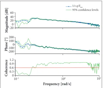
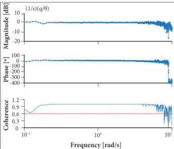
Based on data acquired from the longitudinal and lateral cyclic control inputs, in level light at 80 KIAS, the angular compatibility, in the frequency domain, between angular rates and attitudes, multiplied by an integrating element (1/s) for the longitudinal and lateral axes, respectively, are presented in Figs. 7 and 8.
As observed in Figs. 7 and 8, the integrator element (1/s) “cancels” the first-order characteristics of the attitude and angular rate relation, i.e. Bode diagrams featuring a constant response in magnitude and phase are also constant and equal to 0°. Fitting the frequency responses presented, it is obtained a Kvalue close to unity (1.022, for longitudinal axis, and 1.045, for lateral axis) and practically zero effective time delay (0.058 s, for longitudinal axis, and 0.055 s, for lateral axis). Then one verifies the kinematic compatibility of the channels employed to flying qualities analysis, with a correct sign convention and the conversion to the units of measurement of interest held.
It must be emphasized that the results described are valid in the range in which the coherence function has no oscillatory behavior and its value is greater than 0.6, i.e. from 0.08 to 6.15 rad/s, for the longitudinal control input, and 0.03 to 8.49 rad/s, for the lateral control. This reference value for coherence function provides a signal-to-noise ratio and random error within acceptable levels (Tischler and Remple 2012). Further details and more emphasis on the interpretation of the results using the coherence function will be presented in the frequency-domain results.
In additionprimarily, the FTI employed does not have, as mentioned, the purpose of veriication the lying qualities requirements employing frequency-domain techniques. Also,
-10 -20 0 10
M
ag
ni
tud
e
[dB
]
-400 -300 -200 -1000 100
P
h
as
e
[º]
10–1
100 101
0 0.3 0.6 0.9 1.2
C
o
he
re
n
ce
Frequency [rad/s]
(1/s)(q/θ)
-10 0
10 (1/s)(p/ϕ)
M
agn
it
ud
e
[d
B]
-100 -50 0 50
P
h
ase
[
º]
10–1 100 101
0 0.3 0.6
0.9
1.2
C
oh
er
en
ce
Frequency [rad/s]
Figure 7. Frequency-domain angular consistency – longitudinal axis.
the detailed information of the dynamic characteristics of sensors and ilters are not available, so the next stage of the data post-processing, referring to the iltering, cannot be applied.
During the initial inspection of the data one observes: an absence of too noise signals; no problem on the sampling rate; and lack of knowledge about sensors characteristics, in order to all of them be iltered as the same. hus, given the results obtained in the visual inspection phase and angular consistency, for the purposes of this paper, the instrumentation characteristics and, consequently, the acquired data were considered appropriate without any correction in the sampling rate before the spectral analysis.
SPECTRAL ANALYSIS
From the study of dynamical systems, given an ideal physical system single input-single output (SISO) — physically realizable, characteristic parameters constant (time invariable), stable and linear (Bendat and Piersol 1980) — excited by a sinusoidal force function with frequency(ω = 2πf), its properties lead to a particular and a general solution. Ater a period of time, the general solution, transient, is damped and remain, in steady state, the particular solution, whose response depends uniquely on the external force.
The response of this system is also characterized as a sine function with the same frequency (irst harmonic) of the force function (input); the response has magnitude and phase relative to the input, modiied by the intrinsic characteristics of the system and by means of the frequency input itself.
he analysis of the system frequency response, H(f), of this simpliied example that can be extended for any input and output, periodic, non-periodic (deterministic or random) or stationary random data, is the evaluation of the magnitude ratio of the input-output relation and the phase relation over a frequency spectrum. Once it is possible to extend the problem to physical systems with realistic features, H(f) describes the system dynamic behavior, sometimes nonlinear, in terms of the best linear description of the input-output behavior,
i.e. the irst harmonic descriptive function, without imposing any prior knowledge of their internal structure, order, or equations of motion (Tischler and Remple 2012).
Mathematically, the frequency response, H(f), is a complex function, characterized by its gain factor (|H(f)|) and phase delay (<H(f)), which relates the system output and input inite Fourier transform (Fourier coeicient, Y(f) and X(f), respectively), for each frequency f.
When one employs light test data obtained from frequency-domain scope, the Fourier coefficients are obtained using the Discrete Fourier Transform (DFT), for the signals exist only in a inite-time interval, with a sampled data in a certain rate (ωs = 2π/Δt), for a recording with total duration of NΔt, where N is the number of discrete points of frequency (Bendat and Piersol 1980). hey are calculated at points oten equally distributed from the minimum resolution (ωmin= Δω = 1/NΔt) to the sampling rate.
With the Fourier coeicients it is possible to determine other important one-sided spectral functions, also called spectral density functions: the input autospectrum (Gxx), or input power spectral density (PSD), which represents the excitation density of power as a function of frequency; the output autospectrum (Gyy), or output PSD, which represents the response power distribution as function of frequency; and cross spectrum (Gxy), or cross PSD, which represents the power transfer from input to output, as a function of frequency, which contains the magnitude and phase information from the Fourier coeicients (Tischler and Remple 2012).
The spectral functions are used directly to evaluate the frequency content of the excitation and the aircrat response for a particular identiication maneuver. Its use in data analysis allows the selection of the most appropriate test runs to be concatenated, veriication of turbulence levels, frequency sweep irregularities and inding the real uniformly excited frequency spectrum.
Using the simpliied Fourier analysis, erroneous frequency information appears as side lobes of Fourier frequency of interest. his phenomenon, known as “leakage”, permits the “leakage” of power at frequencies far from the central lobe and introduces signiicant abnormalities on spectral functions estimates, particularly for sinusoidal data samples (Bendat and Piersol 1980). To reduce it the technique employed is called windowing, with overlapping windows or periodograms, which produces smoother spectral estimated using the average of multiple segments of data (Tischler and Remple 2012) and reduces their random errors.
frequencies usually limited to the length of 50% Trec (Tischler and Remple 2012).
On the other hand, the greater the number of windows, the larger the division of the total time interval, minimizing random error due to the larger sample for taking averages. In joining two or three recorded intervals of data one achieves a recording interval concatenated (TF) of suitable length that allows the accuracy at low frequencies (function of Trec) allied to the major capacity of segment division. It is generally recommended that Twin be less than 20% TF (Tischler and Remple 2012).
hus, selecting the width of the window involves a compromise between a smaller random error and a better identiication of the lower frequency content (Williams et al. 1995). Even with an iterative process for its optimization, whose can show itself laborious, no single window size selection can produce a good result over the entire frequency range of interest. To obtain the most accurate identiication estimates for a particular situation, the spectral calculations would have to be performed repeatedly, in an automatically matter, using several diferent window sizes, merging the results obtained. This technique, also called as composite windowing, is not employed in the present research.
Once the temporal history is divided in segments, data of each window segment are weighted by a window function (w(t)). hus, it minimizes the “weight” of the beginning and end of each segment, avoiding the “leakage” caused by the addition of spurious dynamics during the data segmentation process (Tischler and Remple 2012). Several distinct functions are employed for this purpose as the half-sine or the Hanning window. Employing this method the spectral functions are now smoothly estimated and the frequency response function for SISO systems can be directly obtained.
Figures 9 and 10 represent, respectively, the longitudinal and lateral control inputs when concatenated, based on runs 1, 2 and 3 of Figs. 1 and 2.
Based on Fig. 9 one can observe that, for longitudinal cyclic control inputs, the inputs when concatenated provide an interval of 530 s. Likewise, based on Fig. 10, for lateral cyclic control inputs, the concatenated total time is 648 s. hus, for this research, following the recommendations previously described herein, one selects: Twin of 53 s, for data on the excitation of longitudinal input, and Twin of 65 s, for the lateral input.
For non-linear systems analysis, as interpreted by Tischler and Remple (2012), the frequency response is descriptive, since it measures the output portion linearly related to the input. hus, it is an equivalent linear model that minimizes the mean square diference
Figure 9. Concatenated longitudinal control inputs – level light (80 KIAS).
0 50 100 150 200 250 300 350 400 450 500 -2.5
-2 -1.5
-1 -0.5
0 0.5
Time [s]
бion
[
in]
0 100 200 300 400 500 600
–2 –1 0 1 2 3
Time [s]
бlat
[in]
Figure 10. Concatenated lateral control inputs – level light (80 KIAS).
between the current response signal and its approach by the irst harmonic. he non-linear efects that are not characterized by the function are associated with higher order harmonics of the expansion of Fourier series. hese harmonics appear as noise in the response measurement. Typically, the vast majority of nonlinear efects is iltered by the low-pass nature of the rotary-wing aircrat dynamics.
However, a way to measure the quality of this linear approximation by the irst harmonic is the coherence function (γ2
xy ), deined as Eq. 1:
where: Gxx is the input PSD; Gyy is the output PSD; and Gxy
is the cross PSD.
(1)
γ ˆ2
xy( f ) =
| G ˆxy( f )
|
2he function deined by Eq. 1 measures the portion of Gyy
linearly attributable to Gxx, for a given frequency (Tischler and Remple 2012); its values range from 0 to 1, where the unit represents perfectly linear systems with noise free spectral estimates.
In practical terms, though, the coherence function exhibits values below unit, primarily due to three reasons. First, in certain systems, nonlinearity cannot be neglected or described simply by the first harmonic. This is the basis for the use of small perturbations and small excitation amplitudes, knowing that this is difficult to be met in rotary-wing aircraft, especially in hovering flight, when low-frequency control inputs are present.
A second common cause for the coherence reduction is the output or input noise on the measured signal (measurement noise). hough not contributing or not afecting directly the light control input or the response of the aircrat, this type of noise contaminates the recorded signal and hence causes errors in the frequency response estimate (Williams et al. 1995). For this reason, once more, the importance of using high-quality sensors for light control inputs which ideally free noise must be emphasized. Regardless of the correlation with the measured signal or with the own signal (output or input) in which the noise is present, always there are random errors (dispersion of the spectral estimate around an expected value) that are relected in the coherence function. his error can be minimized and spectral accuracy signiicantly improved for a certain level of coherence, when the concatenation method is employed, for the normalized random error is inversely proportional to the average number of independent data intervals (Williams et al. 1995).
he third source of reduction of coherence is the existence of additional, secondary and not measured inputs in the system. hey come from gusts, turbulence or other source of process noise, or secondary control inputs acting in not-excited axes arising from the pilot himself or some aircrat automatic control system function kept active, e.g. the SAS (Williams et al. 1995). hus, to prevent the reduction of coherence due to those noise errors, the recommendations to realize frequency sweep tests in minimal wind conditions and low atmospheric turbulence must be implemented. Accordingly, recommendations involving: (a) action in the non-excited controls to maintain the light condition around a trimmed reference; (b) amplitude; and (c) non-correlation of the entrances on non-excited controls to the proper excitation, are almost inevitable in helicopter light test analyses.
STANDARD COMPLIANCE
Usually, the Bode diagrams are used to present the results of the light data frequency response function, i.e. magnitude in dB (dB = 20 × log10|H(f)|) and phase (e.g. in rad/s) versus frequency in a logarithmic scale. he properties and characteristics of the Bode diagrams allow easier treatment of the data, for they are additives for serial systems and able to present responses on the same graphic involving a wide frequency range, from the lowest to the highest.
he shape of the magnitude and phase curves on Bode diagrams, speciically the gradient of the magnitude curves and the phase shit, are indicative of the system structure: number of poles and/or zeros and cutof frequencies. he existence of peaks in these igures are also interpreted as due to the natural system modes, and the frequency in which they occur, indicating an oscillatory response, allowing the estimates of its natural frequency and damping ratio.
Bode diagrams in Figs. 11 and 12 of the open-loop system’s SISO relationship show magnitude, phase along with coherence for the longitudinal and lateral axes excitation, respectively. Since the attitudes and angular rates signals have diferent behavior and quality throughout the frequency range, the former being most used at low frequencies and the latter, for high frequencies of the spectrum. For this reason, the response in Bode diagrams employ the integration of the angular rate signal, what showed more wide frequency range in terms of best coherence. he angular consistency analysis between these two signals validates their use.
Figures 11 and 12 also show the 95% conidence levels of the frequency response, based on the normalized random error function, as given by Bendat and Piersol (1980).
The first important aspect to be noticed in Figs. 11 and 12 is the frequency range in which the data present coherence higher than the reference value (0.6), showing no oscillatory behavior or sudden drops. For the longitudinal axis excitation, it can be found in the range of 0.28 to 4.03 rad/s, while, for the lateral axis’s, 0.1 to 14.90 rad/s. For frequencies not included in these ranges there are loss of coherence, be by the higher order dynamics of the aircrat and thus intrinsic to the system or due to the measurement or process noise from data acquisition system or in the data acquisition process. The latter is the main reason of the observed efects in this research.
-20 0 20 40 60
Magnitude [dB]
1/s q/δ ion
95% confidence levels
-200 -100 0 100 200
Phase [°]
10–1 100 101
0 0.3 0.6 0.9 1.2
Coherence
Frequency [rad/s]
-50 0 50
Magnitude [dB]
-400 -300 -200 -100 0
Phase [°]
10–1 100 101
0.3 0 0.6 0.9 1.2
Coherence
Frequency [rad/s]
1/s pδ lat
Confidence levels Figure 11. Bode diagram and coherence function for longitudinal cyclic input.
(irst order) can characterize the dominant dynamics modes of the tested aircrat. Furthermore, this equivalent model allows anticipating some model structure characteristics and dynamic modes (Tischler and Remple 2012).
Moreover, stability in closed-loop can be inferred by means of the Bode diagram using the gain margin (GM), deined as the permissible increase in closed-loop gain, before the system becomes unstable (Steven and Lewis 2003) and phase margin (PM), amount of phase that exceeds −180° (Steven and Lewis 2003). For piloted closed-loop systems, changes in the piloting gain afect stability, deining a corresponding phase
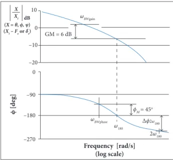
delay (Williams et al. 1995). Because the gain margin can be interpreted as a measure of the pilot’s allowable gain increase without it threatens stability. hus, for lying qualities applications, the information from the Bode diagram is a measurement of pilot’s workload. It allows designing the light control systems. For lateral and longitudinal axis, the requirements to be check come from the ADS-33E-PRF (2000) standard, speciically paragraphs 3.4.1.1 Short-term response (bandwidth) and 3.4.6.1 Small-scale roll attitude response to control inputs (bandwidth), which employ frequency-domain parameters obtained from the Bode diagrams: bandwidth frequency (ωBW), and phase delay (τp).
he bandwidth frequency is the lower closed-loop frequency of the angular attitude response to a pilot control input, which ensures, at least, 6 dB of gain margin (ωBWgain) or 45° of phase margin (ωBWphase) from the frequency of neutral stability (ADS-33E-PRF 2000). Essentially, ωBW is a measure of the quickness at which the aircrat responds to a control input by setting the maximum input frequency that result in a useful response, from magnitude and phase point of view. In addition, as deined in ADS-33E-PRF (2000), ωBW is the maximum frequency that a pilot employing pure gain control strategy reaches a valid igure of merit, without afecting the stability. When an aircrat allows a pilot to employ, as control strategy, a pure gain element which does not require phase compensation, so-called synchronous control, the workload is minimized, reaching, for certain tasks, the bests HQR. For helicopters, greater workload tasks (also referred to as high-gain tasks) are directly afected, such as precision hover, pirouette, slope landing and ofset running landing (Tischler and Remple 2012).
he phase delay is determined from the frequency at which the phase is equal to −180° (ω180) and the value of the phase (φ2ω180) measured in this double (2ω180), as Eq. 2:
Figure 12. Bode diagram and coherence function for lateral cyclic input.
As one can observe in Eq. 2, because there are data accuracy and coherence in this frequency range, the parameter is the slope of the phase curve at the point where the output delays 180° with respect to the input (neutral stability). As the pilot increases the gain in a certain task, he (she) approaches the frequency at which the aircrat responds out-of-phase with respect to the input. he pilot’s natural reaction is to apply, mentally, a lead ilter to compensate the phase lag. he success of this technique
(2)
τ
p φ2ω180 + 180o
depends on the response predictability, measured by the phase lag: greater frequency changes will cause greater phase shits, which turns response less predictable and more susceptible to pilot induced oscillations (PIO).
he ωBW and the characteristic points to obtain τp (ω180, ϕ2ω180 and 2ω180), as deined in the ADS-33E-PRF (2000) standard, are shown in Fig. 13, which represents the Bode diagrams of the ratio between the angular attitude and the input, measured as light control displacement (δs) or light control load (Fs).
Comparison with the reference values of ADS-33E-PRF (2000) standard can be done based on linear interpolation of the Bode diagrams (Figs. 11 and 12) around the desired parameters. Furthermore, the uncertainties of the presented results are based on the 95% conidence interval in magnitude and phase. In this case, it can be noticed that, once the normalized random error is a function of coherence, to γ 2
xy values close to unity, smaller errors and, consequently, smaller ranges of conidence are achieved, making them practically imperceptible in the shown curves.
For the longitudinal cyclic excitation, within the frequency range in which there is acceptable coherence, it is not possible to identify the phase of 2ω180(6.934 rad/s), thus preventing the calculation of the phase delay, applying Eq. 2. Table 1 summarizes the characteristic parameters found in the longitudinal response of the helicopter, at level light (80 KIAS).
Even without the information regarding the phase delay, the bandwidth frequency already provides useful knowledge on pilot demands in carrying out tasks in closed-loop, applying HQR.
Since this frequency is the maximum in which the pilot is able to close the loop by means of synchronous control and achieve adequate stability, its relationship to the cutof frequency (ωco), for a particular task, is a measure of the easiness with which the task is to be performed. Usually, tasks that require precise regulation associated with high pilot compensation gains result in increase of ωco. If it exceeds ωBW, it requires that the pilot imposes a phase delay control strategy to achieve the stability margin needed to close the control loop with adequate damping. hus the bandwidth frequency is usually designed to be as high as possible, a requirement for an adequate light control system. For the lateral cyclic excitation, 2ω180 (13.842 rad/s) lies within the frequency range in which the coherence is acceptable, allowing the deinition of phase delay. Table 2 summarizes the ADS characteristic parameters for helicopter lateral response in level light (80 KIAS).
Once obtained both parameters of interest, the ADS standard speciies the regions wherein the aircrat reaches a certain predicted level of lying qualities from the level 1, which is satisfactory in quickness and accuracy, not requiring modiications, to level 3, wherein the lying qualities are degraded, requiring improvements. he regions and hence the levels to be achieved, depends on the operating task to be performed
ωBWgain
ωBWphase ω180
2ω180
∆ϕ2ω180
GM = 6 dB 0
10
–10
–20 0
–90
–180
–270
Frequency [rad/s] (log scale)
ϕ [d
eg]
ϕM = 45o
(X = θ, ϕ, ψ) (Xi – Fs or бs)
X
dB
Xi
Figure 13. Deinitions of ωBW and τp (ADS-33E-PRF 2000).
Characteristic parameter
Frequency (rad/s)
Uncertanty (rad/s)
ω180 3.467 ±0.030
ωBWphase 1.612 ±0.008
ωBWgain 2.588 ±0.023
ωBW 1.612 ±0.008
Table 1. AS355-F2 level light (80 KIAS) longitudinal lying qualities ADS parameters.
Characteristic
parameter Value Uncertanty
ω180 6.921 rad/s ±0.012 rad/s
ωBWphase 2.013 rad/s ±0.003 rad/s
ωBWgain 4.430 rad/s ±0.012 rad/s
ωBW 2.013 rad/s ±0.003 rad/s
φ2ω180 −231.04° ±1.1°
τp 0.013 s ±0.001 s
Figure 14. Flying qualities levels – AS355-F2 longitudinal response (ADS-33E-PRF 2000).
0.4
0.3
0.2
0.1
0
τpϕ
[s]
0.4
0.3
0.2
0.1
0
τpϕ
[s]
0.4
0.3
0.2
0.1
0
0 1 2 3 4 5
τpϕ
[s]
ωBWϕ[rad/s]
(a) Target acquisition
and tracking
AS344-F2
Level 3
Level 2
Level 2
Level 2 Level
3
Level 3
Level 1
Level 1
Level 1
(b) All other MTEs —
VMC and Fully Attended Operations
(c) All other MTEs — IMC and/or Divided Attention Operations
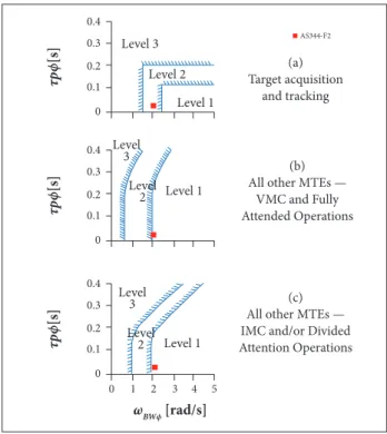
Figure 15. Flying qualities levels – AS355-F2 lateral response (ADS-33E-PRF 2000).
0.4
0.3
0.2
0.1
0
τpϕ
[s]
0.4
0.3
0.2
0.1
0
τpϕ
[s]
0.4
0.3
0.2
0.1
0
0 1 2 3 4 5
τpϕ
[s]
ωBWθ[rad/s]
(a) Target acquisition
and tracking AS355-F2
Level 3
Level 2
Level 2
Level 2 Level 3
Level 1
Level 1
Level 1
(b) All other MTEs —
VMC and Fully Attended Operations
(c) All other MTEs — IMC and/or Divided Attention Operations by a particular aircrat (Mission Task Elements, MTE) and the operating environment in which they will be executed, considering the visual acuity (Good Visual Environment, GVE or Degraded Visual Environment, DVE), weather condition (Visual Meteorological Conditions, VMC or instrument meteorological conditions, IMC), attention, among other factors.
he level light pitch responses for the AS355-F2 aircrat are shown in Fig. 14 along with ADS-33E-PRF (2000) regions and lying qualities levels. To a wide range of phase delay values, results found permit to classify the aircrat as ADS level 1 only in tasks that did not demand great precision, in visual light conditions and with all attention focused (Fig. 14b), mainly because of the low ωBW obtained.
For the lateral response, involving the target acquisition and tracking maneuver (Fig. 15a), high gain task that requires precise regulation of the pilot in the control loop, the aircrat is classiied as ADS level 2, meaning that its light qualities, for tasks of this nature, exhibit deiciencies which require improvements (speciically, the high value of bandwidth frequency). he result is consistent with closed-loop pilots assessments at high gain tasks (e.g., lateral change in target acquisition), in which is commonly reported moderate workload and small amplitude and high frequency corrections in the lateral cyclic control, with occurrence of overshoots for reacquiring a target.
For all other tasks (Fig. 15b and c), whether in visual or instrument light conditions, with full or partial attention, the aircrat is classiied as ADS level 1, given the low phase delay value, ensuring predictability to the light.
CONCLUSION
his work describes the key aspects of the management process to apply the frequency response methodology to characterize the dynamics of a rotary-wing aircrat, analyze its lying qualities and verify the adequacy of this aircrat to the ADS-33E-PRF (2000) standard.
hroughout the work, all the management process steps required for planning, acquisition and data analysis for frequency sweep light tests are presented, and, when it is possible, exempliied with real light test data from longitudinal and lateral frequency sweep, on level light at 80 KIAS, of AS355-F2 helicopter.
It begins with the design of the instrumentation, deining the parameters that would be acquired, the need to acquire redundant signs and the sensors speciication (their accuracy, sampling rates and iltering).


![Figure 9. Concatenated longitudinal control inputs – level light (80 KIAS).050 100 150 200 250 300 350 400 450 500-2.5-2-1.5-1-0.500.5Time [s]бion [in] 0 100 200 300 400 500 600–2–10123 Time [s]бlat [in]](https://thumb-eu.123doks.com/thumbv2/123dok_br/18889687.424716/13.892.461.808.148.388/figure-concatenated-longitudinal-control-inputs-level-light-kias.webp)