American Journal of Applied Sciences 5 (11): 1429-1432, 2008 ISSN 1546-9239
© 2008 Science Publications
Corresponding Author: Reza Kamyab Moghadas, Iranian Academic Center for Education, Culture and Research, Kerman, Iran
1429
Prediction of Double Layer Grids’ Maximum Deflection Using Neural Networks
1
Reza Kamyab Moghadas,
2Kok Keong Choong
1
Iranian Academic Center for Education, Culture and Research, Kerman, Iran
2
School of Civil Engineering, Universiti Sains Malaysia, Penang, Malaysia
Abstract: Efficient neural networks models are trained to predict the maximum deflection of two-way on two-way grids with variable geometrical parameters (span and height) as well as cross-sectional areas of the element groups. Backpropagation (BP) and Radial Basis Function (RBF) neural networks are employed for the mentioned purpose. The inputs of the neural networks are the length of the spans, L, the height, h and cross-sectional areas of the all groups, A and the outputs are maximum deflections of the corresponding double layer grids, respectively. The numerical results indicate that the RBF neural network is better than BP in terms of training time and performance generality.
Key words: Backpropagation, radial basis function, neural networks, maximum deflection, double layer grids
INTRODUCTION
Many thousands of impressive space structures have been built all over the world for covering sport stadiums, gymnasiums, leisure centers, aircraft hangars, railway stations and many other purposes. A number of these structures have spans of well over 200m. Due to their three dimensional action, space structures are very efficient structural systems to carry heavy loads as well as to span large distances. As the use of space structures becomes more and more popular, it is essential to evolve strategies for their convenient analysis and design. In the present investigation, neural network techniques are employed for this purpose. Over the last decade, artificial intelligence techniques have emerged as a robust tool to replace time consuming procedures in many scientific or engineering applications. The use of neural networks to predict finite element analysis outputs has been studied previously in the context of many engineering applications[1-5]. The principal advantage of a properly trained neural network is that it requires a trivial computational effort to produce an approximate solution.
The main aim of the present study is to train neural networks for predicting the maximum deflection of double layer grid space structures for static loadings. The double layer grids considered are way on two-way and the bar elements are connected by MERO type of joints. The length of the spans, L and the height, H, of the space structures are variable. Due to the practical demands, members are grouped. In this work, three
groups are considered. That is, all the top, web and bottom layer elements are grouped in groups 1 to 3, respectively. Cross-sectional areas of the all groups, A, are selected from a list of available tube sections in STAHL. In the present study, the inputs of neural networks are the length of the spans, L, the height, H and cross-sectional areas of the all groups, A, while the outputs are maximum deflections of the corresponding double layer grids. In the present study, backpropagation (BP) and Radial Basis Function (RBF) networks are employed. Fundamental concepts of BP and RBF networks are briefly explained as follows.
Backpropagation neural network: The most popular and successful learning method for training the multilayer neural networks is the backpropagation algorithm. The development of the Backpropagation learning was reported by Rumelhart Hinton and Williams[6]. The algorithm employs an iterative gradient-descent method of minimization which minimizes the mean squared error between the desired output and network output. The backpropagation training procedure is presented below.
N M 2 i j 1 i 1 1
E e ( n )
2 = =
= (1)
N, M and n are number of training input patterns, dimension of output space and number of iterations, respectively.
(L)
i i i
Am. J. Applied Sci., 5 (11): 1429-1432, 2008
1430 N
l (l) ( l 1)
i ij j
j 1
v ( n ) w y − ( n )
=
= (3)
where ( l 1) j
y − ( n )is the function signal of neuron j in the previous layer (l-1) at iteration n. (l)
ij
w ( n ) is the weight of neuron i in layer l that is fed from neuron j in layer (l-1).
Then the output signal of neuron i in layer l is
l l
i i
y ( n )=f ( v ( n )) (4)
where, f (.) is the activation function.
If neuron i is in the first hidden layer (l = 1), then set 0
i i
y ( n )=x ( n ).
Backward computation (local gradients)
i i
i E ( n )
v ∂ = −
∂ (5)
is called the local error or local gradients. Equation (5) can be simplified to
for neuron i in output layer L:
L L L
i( n )=e ( n ) f ( v ( n ))i ′ i (6) for neuron i in hidden layer l:
l l ( l 1) ( l 1)
i i k ki
k
( n )=f ( v ( n ))′ + ( n ) w + ( n ) (7) where, f′(.) is the derivative of the activation function with respect to v(n).
If the activation function is chosen to be the hyperbolic tangent function, then f′(.) is:
2 i
i i
i d f ( v )
f ( v ) (1 f ( v ))
d v
′ = = − (8)
Hence, adjust the weights of the network in layer l according to the generalized delta rule:
( l ) ( l ) ( l ) ( l 1)
ij ij i j
w ( n 1)+ =w ( n )+ ( n ) y − ( n ) (9)
where, µ is the positive constant learning rate, usually equals to 0.01.
If after updating the weights, the error E is not minimized, new iterations are required.
Radial basis function neural network: The backpropagation algorithm for the design of a multilayer neural network described earlier may be viewed as a form of stochastic approximation. Radial Basis Functions (RBFs) take a different approach by
viewing the design of a neural network as a curve-fitting problem by finding a best fit to the training data in a multidimensional space. The use of RBF in the design of neural networks was first introduced by Broomhead and Lowe[7]. The RBF network basically involves three entirely different layers; an input layer, a hidden layer of high enough dimension and an output layer. The transformation from the hidden unit to the output space is linear. Each output node is the weighted sums of the outputs of the hidden layer. However, the transformation from the input layer to the hidden layer is nonlinear. Each neuron or node in the hidden layer forming a linear combination of the basis (or kernel) functions which produces a localized response with respect to the input signals. This is to say that RBF produce a significant nonzero response only when the input falls within a small localized region of the input space. The most common basis of the RBF is a Gaussian kernel function of the form:
T
l l
l
l ( x c ) ( x c )
( x ) exp[ ], l 1, 2,..., P
2
− −
ϕ = − = (10)
where, ϕl is the output of the lth node in hidden layer, x is the input pattern,clis the weight vector for the lth node in hidden layer, i.e., the center of the Gaussian for node l, l is the normalization parameter (the measure of spread) for the lth node and P is the number of nodes in the hidden layer. The outputs are in the range from zero to one so that the closer the input is to the center of the Gaussian, the larger the response of the node. The name RBF comes from the fact that these Gaussian kernels are radially symmetric; that is, each node produces an identical output for inputs that lie a fixed radial distance from the center of the kernel cl. The network outputs are given by:
T i i l
y =w ϕ( x ), i=1, 2,...,Q (11)
where, yi is the output of the ith node, wiis the weight vector for this node, Q is the number of nodes in the output layer and ϕl( x ) is the vector of outputs from the hidden layer (augmented with an additional component or a bias which assumes a value of one).
To train the hidden layer of RBF networks no training is accomplished and the transpose of training input matrix is taken as the layer weight matrix[7].
T =
C (12)
Am. J. Applied Sci., 5 (11): 1429-1432, 2008
1431 In order to adjust output layer weights, a supervised training algorithm is employed. If for each input vector Xiin the training set, the outputs from the hidden layer are made a row in a matrix , target vectors Tiare placed in corresponding rows of target matrix T and each set of weights associated with an output neuron is made a column of the matrix W, training consists of solving the following matrix equation[7]:
1
−
= =
T W W T (13)
Matrix is, in general, not square, it is not invertible, only its pseudo inverse can be found by singular value decomposition (SVD) method[7].
In order to design neural networks MATLAB[8] is employed. In order to produce the training set a computer program is developed. The structural analysis is based on the finite element formulation of the displacement method.
RESULTS AND DISCUSSION
The space structure model selected is described. Then, some information about data selection and the neural networks training are provided.
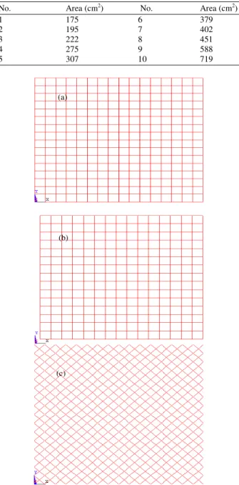
Model description: The double layer grid considered is the type of two-way on two-way and the bar elements are connected by MERO type of joints. Each span contains 15 bays of equal length in both directions. The structure is assumed to be supported at corners of bottom layer each on three nodes. The double layer grid is shown in Fig. 1. The length of the spans, L, is varied between 25 and 75 m with the steps of 5 m. the height, h, is varied between 0.035 and 0.095 L with the steps
Fig. 1: Double layer grids (two-way on two-way)
of 0.2 m. Due to the practical demands, members are grouped. Cross-sectional areas of the all groups, A, are selected from a list of available tube sections in STAHL given in Table 1. In this work, three element groups are considered. That is, all the top, bottom and web layer elements are grouped in groups 1 to 3, shown in Fig. 2, respectively. The sum of dead and live load equal to 250 kg m−2 is applied to the nodes of the top layer.
Table 1: Available cross-sectional areas
No. Area (cm2) No. Area (cm2)
1 175 6 379
2 195 7 402
3 222 8 451
4 275 9 588
5 307 10 719
(a)
(b)
(c)
Am. J. Applied Sci., 5 (11): 1429-1432, 2008
1432
Data selection and neural networks training: Inputs of the neural networks are the length of the spans, L, the height, h and cross-sectional areas of the all groups, A1, A2, A3, while the outputs are maximum deflections
of the corresponding double layer grids.
{
}
T{
max}
1 2 3
IV= L h A A A , OV= (14)
where, IV and OV are input and output vectors, respectively. Also, max
represents the maximum deflection of the double layer grids.
Backpropagation (BP) and Radial Basis Function (RBF) neural networks are employed. In order to provide the training set a computer program is developed. In this program, the randomly produced double layer grids are analyzed and their maximum deflections are saved as the output vectors components. The structural analysis is based on the finite element formulation of the displacement method. As the size of problem is very large, a training set including 3500 samples is produced. From which, 3000 and 500 samples are selected to train and test the performance generality of the neural networks, respectively. The results of testing performance generality of the BP and RBF neural networks are summarized in Table 2. Error percentages of the neural networks in testing phase are also shown in Fig. 3, 4.
0 5 10 15 20 25 30 35
1 101 201 301 401 501
Test samples number
E
rr
o
r
(%
)
Fig. 3: Errors of BP network in test phase
0 5 10 15 20 25 30 35
1 101 201 301 401 501
Test samples number
E
rr
o
r
(%
)
Fig. 4: Errors of RBF network in test phase
Table 2: Available cross-sectional areas
Network Training time (sec) Max Error (%) Mean Error (%)
BP 492.50 34.693 4.982
RBF 47.72 14.304 2.554
CONCLUSION
Efficient neural networks are trained to predict the maximum deflection of two-way on two-way grids. The elements of the double layer grids are divided into three groups. Span, height and cross-sectional areas of the double layer grids are taken into account as the inputs of the neural networks. The outputs are chosen to be the maximum deflection of the structures. It is obvious that, with mentioned inputs, the size of the problem becomes very large. In order to attain accurate prediction, a large training set is required. Therefore, 3500 samples are generated on a random basis and 3000 and 500 ones are selected for training and testing, respectively. Two well known neural networks, Backpropagation (BP) and Radial Basis Function (RBF) are trained for the mentioned purpose. The numerical results demonstrate efficiency of the both networks. Also, it is observed that the RBF is better than BP in terms of training time and approximation errors.
REFERENCES
1. Hajela, P. and L. Berke, 1991. Neurobiological computational models in structural analysis and design. Comput. Struct., 41: 657-667.
2. Berke, L., S.N. Patnaik and P.L.N. Murthy, 1993. Optimum design of aerospace structural components using neural networks. Comput. Struct., 48: 1001-1010.
3. Theocharis, P.S. and P.D. Panagiotopoulos, 1993. Neural networks for computing in fracture mechanics: methods and prospects of applications. Comput. Methods Applied Mech. Eng., 106: 213-228.
4. Adeli, H. and P. Hyo Seon, 1995. Optimization of space structures by neural dynamics. Neural Networks, 8 (5): 769-781.
5. Topping, B.H.V. and A. Bahreininejad, 1997. Neural computing for structural mechanics. UK: Saxe Coburg.
6. Haykin, S., 1994. Neural Networks: A Comprehensive Foundation, Macmillan, New York, NY.
7. Wasserman, P.D., 1993. Advanced Methods in Neural Computing, New York: Prentice Hall Company, Van Nostrand Reinhold.