Azormod dynamic general equilibrium model for Azores

(1)

WORKING PAPER SERIES

CEEAplA WP No. 02/2009

Azormod Dynamic General Equilibrium Model

for Azores

Mário Fortuna Ali Bayar Cristina Mohora Masudi Opese Suat Sisik March 2009

(2)

Azormod Dynamic General Equilibrium Model for

Azores

Mário Fortuna

Universidade dos Açores (DEG)

e CEEAplA

Ali Bayar

Universite Libre de Bruxelles

Departement D’Economie Appliquee

EcoMod

Cristina Mohora

Universite Libre de Bruxelles

Departement D’Economie Appliquee

EcoMod

Masudi Opese

Universite Libre de Bruxelles

Departement D’Economie Appliquee

EcoMod

Suat Sisik

Universite Libre de Bruxelles

Departement D’Economie Appliquee

EcoMod

Working Paper n.º 02/2009

Março de 2009

(3)

CEEAplA Working Paper n.º 02/2009 Março de 2009

RESUMO/ABSTRACT

Azormod Dynamic General Equilibrium Model for Azores

The main objective of this paper is to present a multi-sectoral, multi-regional dynamic modelling platform of the Azores economy integrated within the European and global context. The platform will have the highest capabilities of analysis and forecasting in Azores for problems related to structural sectoral and regional issues, agriculture, labour markets, public finance, trade, EU funds, regional development, environment, and energy. The modelling platform is intended to act as an analytical and quantitative support for policy-making.

Mário Fortuna

Departamento de Economia e Gestão Universidade dos Açores

Rua da Mãe de Deus, 58 9501-801 Ponta Delgada Ali Bayar

Universite Libre de Bruxelles

Departement D’Economie Appliquee Avenue Paul Heger 2

B-1000 Bruxelles Cristina Mohora

B-1000 Bruxelles Masudi Opese

B-1000 Bruxelles Suat Sisik

(4)

AZORMOD

DYNAMIC GENERAL EQUILIBRIUM MODEL FOR

AZORES

Mário Fortuna Ali Bayar Cristina Mohora Masudi Opese Suat Sisik

Abstract

(5)

1 Introduction

The current version of the modelling platform of the Azores economy is represented by a dynamic multi-sectoral computable general equilibrium model (CGE), which incorporates the economic behaviour of six economic agents: firms, households, regional government, Mainland government, European Commission and the external sector.

2 Technical overview

The goods-producing sectors, consisting of both public and private enterprises, are disaggregated into 45 branches of activity. Households are divided into six income groups, to analyze the distributional effects of various policy measures. Special attention is paid to the economic links between the regional government, the Mainland government and the European Commission. With regard to the rest of the world the economy is treated as a small open economy with no influence on (given) world market prices. Trade relations are differentiated according to four main trade partners: Mainland, EU, US and the rest of the world. The behaviour of each agent in the model is described in detail below.

The model has been solved by using the general algebraic modelling system GAMS (Rosenthal, 2006).

The following conventions are adopted for the presentation of the model. Variable names are given in capital letters, small letters denote parameters calibrated from the database (SAM) and elasticity parameters. The subscript s stands for one of the production activities (45 branches of activity). The subscript c stands for one of the commodities (45 types of commodities). The subscript qu stands for one of the households’ income groups (6 households’ income groups). The subscript ctm stands for one of the trade and transport services (7 types of trade and transport services), while nctm stands for all the other commodities except trade and transport services (38 types of commodities).

2.1 Firms

CGE models do not take into account the behaviour of individual firms, but of groups of similar ones aggregated into branches. A presentation of the production sectors considered in AzorMod is provided in Table 1.

The usual assumption for such a model is that producers operate in perfectly competitive markets and maximize profits (or minimize costs for each level of output)

(6)

equal average and marginal costs, a condition implied by profit maximization for a constant returns to scale technology.

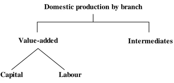
The level of production for each branch of activity is determined from a nested production structure (see Figure 1). In the first stage, producers are assumed to choose between intermediate inputs and value-added according to a Leontief production function. In the second stage, the optimal mix between capital and labour is given by another optimization process, where substitution possibilities between capital and labour are represented by a constant elasticity of substitution (CES) function. Firms’ costs related to corporate income tax and social security contributions are also taken into account in the optimization process.

Figure 1. The nested Leontief and CES production technology for the domestic production by branch of activity

Value-added (KLs) is related to domestic production by branch s (XDs)through a Leontief production function, which assumes an optimal allocation of inputs:

s s s

KL =aKL ⋅XD (1)

where aKLsis the well-known fixed coefficient relating value-added to domestic production. Similarly, total intermediate inputs used by industry s (IOs)are derived as:

,

s c s s c

IO =∑io ⋅XD (2)

where ioc s_, are the technical coefficients. Thus, domestic production valued at basic prices net of taxes ( tp )s but including direct subsidies ( tsp )s on production from the

regional

government and direct subsidies on production from the European Agricultural Guidance and Guarantee Fund (EAGGF) (tspeuea )s , from the Financial Instrument for Fisheries

Guidance (FIFG) (tspeufi )s , from the European Regional Development Fund (ERDF) s

(tspeuer ), from the European Social Fund (ESF) (tspeues )s and from US (tspusa )s , is given

by the sum of value-added (KLs) for branch s valued at basic prices (PKL )s and

intermediate commodities used by sector s valued at the price of the commodities ( )Pc , less subsidies on intermediate consumption (tsic )c,s but including the trade and transport

margins ctm,c,s ctm ctm

(

∑

tcictm ⋅P ) and value-added taxes (vatic_{c s}_, ) on intermediate consumption: Domestic production by branch

Value-added Intermediates

(7)

Table 1: Activity and commodity disaggregation in AzorMod

1 Agriculture, hunting and forestry, logging

2 Fishing

3 Mining and quarrying

4 Production of meat and meat products

5 Processing of fish and fish products

6 Manufacture of dairy products

7 Prepared animal feeds

8 Beverages & tobacco products

9 Fruits, vegetables, animal oils, grain mill, starches

10 Textiles and leather

11 Wood and products of wood and cork

12 Pulp, paper products; publishing and printing

13 Coke, refined petroleum products and nuclear fuel

14 Chemicals and chemical products

15 Rubber and plastic products

16 Other non-metallic mineral products

17 Basic metals and fabricated metal products

18 Machinery and equipment n.e.c.

19 Electrical and optical equipment

20 Transport equipment

21 Manufacturing n.e.c.

22 Electricity, gas, steam and hot water supply

23 Collection, purification and distribution of water

24 Construction

25 Sale, maintenance, repair of motor vehicles and motorcycles

26 Wholesale trade and commission trade, except of motor vehicles and

motorcycles

27 Retail trade, except of motor vehicles and motorcycles

28 Hotels and restaurants

29 Land transport; transport via pipelines

30 Water transport

31 Air transport

32 Supporting transport activities; activities of travel agencies

33 Post and telecommunications

34 Financial intermediation, excluding insurance and pension funding

35 Insurance and pension funding, except compulsory social security

36 Activities auxiliary to financial intermediation

37 Real estate activities

38 Renting of machinery and equipment without operator

39 Computer and related activities; research and development

40 Other business activities

41 Public administration and defence; compulsory social security

42 Education

43 Health and social work

(8)

s s s s s s

s s s s s

c,s s c,s c ctm,c,s ctm c,s

c ctm

PD (1 tp +tsp +tspeuea MUtspeu+tspeufi MUtspeu+tspeuer MUtspeu+ tspeues MUtspeu+tspusa ) XD = PKL KL

{io XD [ (1 tsic ) P + tcictm P ] (1+vatic )}

⋅ − ⋅ ⋅ ⋅

⋅ ⋅ ⋅ +

⋅ ⋅ − ⋅ ⋅ ⋅

∑

(3)

Parameter MUtspeu insures the consistency between the total EU funds provided as

subsidies on production and the EU subsidies on production by branch of activity.

The trade and transport margins are valued at the price (Pctm) of the corresponding service

(trade services or transport services), while tcictmctm,c,s represents the trade and transport

services ctm per unit of intermediate consumption of commodity c by branch s. Value-added is a CES aggregation of capital (KSKs) and labour(LSKs):

1

[ F_s F_s] F_s

s s s s s s

KL =aF ⋅γFK ⋅KSK−ρ +γFL ⋅LSK−ρ − ρ (4)

Minimizing the costs function:

s s s s s s s s

s s s

Cost ( KSK ,LSK ) [PK (1+tk )+d PI] KSK [PL (1+premLSK )

(1+tl /(1 tl ))] LSK

= ⋅ ⋅ ⋅ + ⋅ ⋅

− ⋅ (5)

subject to (4) yields the demand equations for capital and labour:

s s s F F ( F 1) s s s s s s s s KSK = KL {PKL /[PK (1+tk )+d⋅ ⋅ ⋅PI]}σ ⋅γFKσ ⋅aF σ − ₍₆₎ s s s F F ( F 1) s s s s s s s s LSK = KL { PKL /[PL (1+premLSK ) (1+tl /(1 tl ))]}⋅ ⋅ ⋅ − σ ⋅γFLσ ⋅aF σ − ₍₇₎

and the associated zero profit condition:

s s s s s s s s s s

PKL KL = PK (1+tk ) KSK +PL (1+premLSK ) (1+tl /(1 tl )) LSK +DEP PI⋅ ⋅ ⋅ ⋅ ⋅ − ⋅ ⋅ (8)

where PL is the national average wage and premLSK_sis the wage differential of branch s

with respect to the average wage PL, tl_sis the social security contributions rate for

industry s, PKsis the return to capital in branch s, tksis the corporate income tax rate for

branch s, and ds is the depreciation rate in industry s. The depreciation ( DEP )s related to

the private and public capital stock is valued at the investment price index ( PI ). The

elasticity of substitution between capital and labour is given by σFs, where

1 (1 )

s s

F F

σ = +ρ , and γFKs and γFLs represent the distribution parameters corresponding to capital and labour.

Capital is industry specific, introducing rigidities in the capital market. The inter-sectoral wage differential is a parameter derived as the ratio between the wage by branch and the national average wage (Dervis, De Melo and Robinson, 1982). Holding the inter-sectoral wage differentials constant in counterfactual policy simulations introduces rigidities in the labour market.

Each branch of activity in AzorMod produces several types of goods and services. The optimal allocation of domestic production between the different types of commodities is given by a Leontief function:

c s,c s

s

(9)

where XDDEc represents the domestic production of commodity c by different branches,

supplied on the home and foreign markets, XDs is the domestic production of branch s,

and ioCs ,c is a fixed coefficient expressing the volume of production of commodity c by

the industry s per unit of production of industry s. The corresponding zero profit condition is given by:

s s,c c

c

PD =

∑

ioC ⋅PDDE (10)

where PDDEc is the domestic price of commodity c supplied on the home and foreign

markets and PDs is the price index corresponding to domestic production by branch s.

Treated at an aggregate level, firms’ savings are given by a share of the net operating surplus.

2.2 Households

Households are split into six income groups, the first group being the poorest one. The representative household in each income group receives a part of the capital income (net operating surplus), a part of the labour income, unemployment benefits from the Mainland government and other net transfers from the regional and Mainland governments. The representative household in each income group pays income taxes and saves a share of the net income. Household savings by income group qu ( SHqu), are given by:

qu qu qu qu

SH = MPS ⋅ −(1 ty ) YH⋅ (11)

where YHqu is the household income, tyqu is the personal income tax rate and MPSqu the

household propensity to save. Household propensity to save reacts to changes in the after-tax average return to capital, according to:

qu

elasS

qu qu qu qu

MPS = MPSZ ⋅{[ (1 ty− ) PKavr]/[(1 tyz⋅ − ) PKavrZ]}⋅ ₍₁₂₎

where MPSZqu is the benchmark level of the propensity to save, PKavr is the real average

return to capital received by the household, PKavrZ is the benchmark level of PKavr, tyz_qu

is the benchmark level of the personal income tax rate and elasSqu is the elasticity of

savings with respect to after-tax rate of return. Subsequently, household budget disposable for consumption ( CBUD )qu is derived as:

qu qu qu qu

CBUD = (1 ty ) YH− ⋅ −SH ₍₁₃₎

The disposable budget for consumption is allocated between different goods and services according to a Stone-Geary utility function. Maximizing the utility function:

c ,qu

H c ,qu c ,qu c ,qu

c

U ( C )=

∏

( C −µH )α (14)

subject to the budget constraint:

qu c ctm,c,qu ctm c ,qu c,qu c,qu c,qu c ctm

CBUD =

∑

{[P +

∑

tchtm ⋅P ] ( 1 texc⋅ + ) (1+vatc⋅ +tc ) C⋅ } (15)

with: c ,qu c

H 1

α =

(10)

c ctm,c,qu ctm c,qu c,qu c,qu c,qu c ctm,c,qu ctm

ctm ctm

c,qu c,qu c,qu c,qu c,qu qu cc ctm,cc,qu ctm cc ctm

cc,qu

[P + tchtm P ] (1+texc ) (1+tc +vatc ) C = [P + tchtm P ]

(1+texc ) (1+tc +vatc ) H H {CBUD [P + tchtm P ]

(1+texc ) ( µ α ⋅ ⋅ ⋅ ⋅ ⋅ ⋅ ⋅ ⋅ + ⋅ − ⋅ ⋅ ⋅

∑

cc,qu cc,qu cc,qu 1+tc +vatc )⋅µH }

(16)

Consumption of commodity c by income group qu ( Cc ,qu) is valued at purchaser’s prices,

which include trade and transport margins ctm,c,qu ctm ctm

(

∑

tchtm ⋅P ), excise duties ( texc_{c ,qu}),

value-added taxes ( vatcc ,qu) and other taxes on consumption ( tcc ,qu), where Pc is the price

of commodity c net of taxes. The trade and transport margins on private consumption are valued at the prices corresponding to the trade and transport services ( Pctm), where

ctm,c,qu

tchtm represents the quantity of trade and transport services ctm per unit of commodity

c consumed by the income group qu.

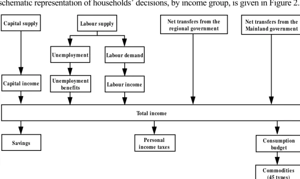
In the allocation process, the consumer first decides on the minimum (subsistence) level of consumption of commodity c ( Hµ c ,qu). Then, the marginal income is allocated between

different types of commodities according to the marginal budget shares ( Hα c ,qu). A

schematic representation of households’ decisions, by income group, is given in Figure 2.

Capital supply Labour supply

Unemployme nt Labour de mand

Une mployme nt

be ne fits Labour income

Capital income Total income Savings Pe rsonal income taxes Consumption budget Net transfe rs from the

regional governme nt

Net transfe rs from the Mainland gove rnme nt

Commoditie s (45 type s)

Figure 2. Decision structure of the representative household by income group

Household welfare gains/losses are valued using the equivalent variation in income

qu

( EV ), which is based on the concept of a money metric indirect utility function (Varian,

1992).

c,qu

qu c ctm,c,qu ctm c,qu c,qu c,qu

ctm c H c,qu qu qu EV = {{[PZ + tchtmz PZ ] (1+texcz ) (1+tcz +vatcz )} / H }α (VU VUI ) α ⋅ ⋅ ⋅ ⋅ −

∑

∏

(17) The indirect utility function (VUqu) corresponding to the Linear Expenditures System

(11)

c,qu

qu qu c ctm,c ,qu ctm c,qu c,qu c,qu

c ctm

c,qu c,qu c ctm,c,qu ctm c,qu c,qu ctm

c H c,qu

VU = {CBUD [P + tchtm P ] (1+texc ) (1+tc +vatc ) H } { H /{[P + tchtm P ] (1+texc ) (1+tc + vatc )}}α µ α − ⋅ ⋅ ⋅ ⋅ ⋅ ⋅ ⋅ ⋅

∑

∏

(18) and the indirect utility function (VUIqu) in the benchmark equilibrium is given by:

c,qu

qu qu c ctm,c ,qu ctm c,qu c,qu c,qu

c ctm

c,qu c,qu c ctm,c,qu ctm c,qu c,qu

ctm c

H c,qu

VUI = {CBUDZ [PZ + tchtmz PZ ] (1+texcz ) (1+tcz +vatcz ) H } { H /{[PZ + tchtmz PZ ] (1+texcz ) (1+tcz + vatcz )}}α µ α − ⋅ ⋅ ⋅ ⋅ ⋅ ⋅ ⋅ ⋅

∑

∏

(19)

where CBUDZqu is the benchmark level of the disposable budget for consumption, PZcis

the benchmark level of the price of commodity c net of taxes, tchtmzctm ,c ,quis the benchmark

level of the trade and transport margin rate, and texczc ,qu, vatczc ,qu and tczc ,quare the

benchmark rates corresponding to excise duties, value-added taxes, and other taxes on consumption, respectively.

Equivalent variation measures the income needed to make the household as well off as she is in the new counter-factual equilibrium (policy scenario) evaluated at benchmark prices. Thus, the equivalent variation is positive for welfare gains from the policy scenario and negative for losses.

2.3 Regional government

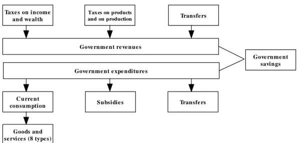
Regional government collects all the taxes, such as: taxes on income and wealth (TRPROP)

and taxes on products and on production (TRPROD) and receives transfers from the

Mainland government, EU funds and transfers from the external sector (TRANSR) (see

Figure 3):

GREV = TRPROP+TRPROD+TRANSR (20)

where GREV stands for the total government revenues.

Figure 3. Structure of the regional government budget

Gove rnme nt re ve nue s

C urre nt

consumption Subsidie s Transfe rs

Gove rnme nt e xpe nditure s

Gove rnme nt savings Goods and se rvice s (8 type s) Taxe s on income and we alth Tax es on products

(12)

The taxes on income and wealth are given by:

qu qu s s s

qu s

TRPROP =

∑

ty ⋅YH +

∑

tk ⋅KSK ⋅PK

(21) In the derivation of each category of tax revenue the tax rate is applied to the

corresponding tax base.

Taxes on products are differentiated in the model according to the category of consumption on which they apply: intermediate consumption, private consumption, and gross capital formation. Taxes on products and on production are provided by:

s s s c ctm,c,qu ctm c,qu

s c ,qu ctm

c,qu c,qu c,qu c,qu c ctm,c ctm c c c ctm

c,s c ctm,c,s ctm c,s c,s s ctm

TRPROD = tp XD PD {[P + tchtm P ] [ texc ( 1 texc ) ( tc +vatc )] C } [P + tcitm P ] vati I

[(1 tsic ) P + tcictm P ] vatic io XD

⋅ ⋅ + ⋅ ⋅ + + ⋅ ⋅ + ⋅ ⋅ ⋅ + − ⋅ ⋅ ⋅ ⋅ ⋅

∑

c c c ,s c c c c c c (tmus PWMUS MUS ERUS)+ (tmrw PWMROW MROW ERROW)

+ ⋅ ⋅

⋅ ⋅ ⋅ ⋅

∑

(22) where Ic represents the investment demand for commodity c, tcitmctm ,c gives the trade and

transport margin rate on investment good c, vatic gives the value-added tax rate on

investment good c, tmusc represents the tariff rate on commodity c coming from US, c

MUS give the imports of commodity c from US, PWMUS_c stands for the import price of

commodity c from US expressed in foreign currency and ERUS is the exchange rate with

respect to the US dollar. Tariff rate on commodity c coming from the rest of the world (ROW) ( tmrw )c is applied to the imports of commodity c from the ROW ( MROW )c ,

valued at the import price expressed in foreign currency ( PWMROW )c , and transformed in

domestic currency using the exchange rate ERROW.

The total transfers received by the regional government (TRANSR) are given by

transfers from the Mainland government ( TRGML ), transfers from EU as direct

subsidies on production ( TRGEC ) and other transfers from EU ( TRGEU ), transfers

from US ( TRGUS ) and transfers from the rest of the world ( TRGW ): TRANSR = TRGML ERML+TRGEU EREU+TRGEC EREU+TRGUS ERUS+ TRGW ERROW

⋅ ⋅ ⋅ ⋅

⋅ (23)

where the transfers are expressed in domestic currency using the exchange rate with respect to Mainland ( ERML ), the exchange rate with respect to EU ( EREU ), the

exchange rate with respect to US ( ERUS ) and the exchange rate with respect to the

rest of the world ( ERROW ).

Regional government expenditures ( GEXP ) comprise the public current consumption ( CGBUD ), total transfers by the government ( TRANS ) and subsidies on products and on

production ( SUBSID ):

GEXP = CGBUD+TRANS+SUBSID ₍₂₄₎

The optimal allocation of the public current consumption between different types of goods and services is given by the maximization of a Cobb-Douglas function:

c

CG

c c

c

(13)

subject to the budget constraint: c c c CGBUD=

∑

P CG⋅ (26) with: c c CG 1 α =

∑

. The maximization of U( CG )c yields the demand equations for public

current consumption by type of commodity:

c c c

P CG = CG CGBUD⋅ α ⋅ (27)

where CGc represents the public demand for commodity c, Pc is the price of commodity c

and αCGc gives the Cobb-Douglas preference parameter corresponding to commodity c.

Total transfers by the regional government include transfers to the households ( TRHG )qu : qu

qu

TRANS =

∑

TRHG ⋅PCINDEX (28)

translated into nominal terms by using the Laspeyres consumer price index ( PCINDEX ).

The total subsidies on products and on production are further derived as:

c,s c c,s s s s

c ,s s

s s s s s s

SUBSID = tsic P io XD [(tsp +tspeuea MUtspeu+ tspeufi MUtspeu+tspeuer MUtspeu+tspeues MUtspeu+tspusa ) XD PD ]

⋅ ⋅ ⋅ + ⋅

⋅ ⋅ ⋅ ⋅ ⋅

∑

(29) The EU funds as direct subsidies on production are transferred to the regional

government budget which allocates them between different branches of activity.

MUtspeuis a scaling parameter which insures the consistency between the total EU

funds and the total subsidies on production distributed to different branches of activity:

s s s s s s

s

TRGEC EREU = MUtspeu⋅ ⋅

∑

[(tspeuea +tspeufi +tspeuer +tspeues ) XD PD ]⋅ ⋅ (30)

The difference between the regional government revenues and the government expenditures yields the government savings ( SG ).

SG = GREV−GEXP₍₃₁₎

2.4 Mainland government

Mainland government collects all the social security contributions, provides unemployment benefits and makes transfers to the households (TRHML )qu and to the

regional government (TRGML).

Social security contributions are derived by applying the social contributions rate ( tl )s

to gross wages. Unemployment benefits received by each household income group are determined by the combination of the replacement rate ( trep ), the national average

wage ( PL ), the total number of unemployed (UNEMP ), and the share of unemployed

subject to unemployment benefits in each household income group (shUNEMPB )qu .

(14)

s s s s qu

s qu

qu qu

SGML = [tl /(1 tl ) LSK PL (1+premLSK )/ERML ] TRHML

(shUNEMPB trep PL UNEMP/ERML ) TRGML

− ⋅ ⋅ ⋅ − − ⋅ ⋅ ⋅ −

∑

(32) 2.5 European Commission

European Commission provides EU funds as direct subsidies to the production sectors

(TRGEC) and other EU funds (TRGEU) to the regional government. The net transfers

by the European Commission to Azores ( SGEC ) are given by:

SGEC = TRGEC TRGEU− − (33)

2.6 Foreign trade

The specification of the foreign trade is based on the small-country assumption, which means that the country is a price taker in both its import and its export markets. Four different trade partners are distinguished in the model: Mainland, EU, US and the rest of the world.

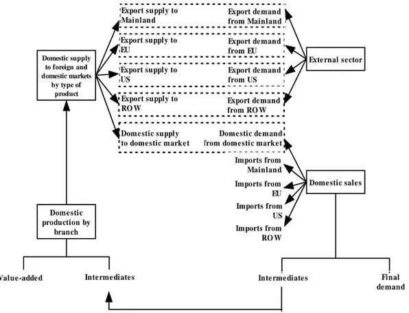
On the import side, imperfect substitution is assumed between domestically produced and imported goods, according to the Armington function (see Figure 4). Thus, domestic consumers use composite goods ( X )c of imported and domestically produced goods,

according to a CES function:

c c c c c c A A A A c c c c c c c c c c A 1 / A c c

X aA ( A1 MML A2 MEU A3 MUS A4 MROW

A5 XDD ) ρ ρ ρ ρ ρ ρ γ γ γ γ γ − − − − − − = ⋅ ⋅ + ⋅ + ⋅ + ⋅ + ⋅ (34)

Minimizing the cost function:

c c c c c c c c c c

c c c c c c

Cost ( MML ,MEU ,MUS ,MROW , XDD ) PMML MML PMEU MEU

PMUS MUS PMROW MROW PDD XDD

= ⋅ + ⋅ +

⋅ + ⋅ + ⋅ (35)

subject to (34) provides the demand for imports from Mainland ( MML )c , the demand for

imports from EU ( MEU )c , the demand for imports from US ( MUS )c , the demand for

imports from ROW ( MROW )c , and the demand for domestically produced goods c ( XDD ): c c c A A ( A 1) c c c c c c MML = X ⋅(P /PMML )σ ⋅γA1σ ⋅aAσ − ₍₃₆₎ c c c A A ( A 1) c c c c c c MEU = X ⋅(P /PMEU )σ ⋅γA2σ ⋅aAσ − ₍₃₇₎ c c c A A ( A 1) c c c c c c MUS = X ⋅(P /PMUS )σ ⋅γA3σ ⋅aAσ − ₍₃₈₎ c c c A A ( A 1) c c c c c c MROW = X ⋅(P /PMROW )σ ⋅γA4σ ⋅aAσ − ₍₃₉₎ c c c A A ( A 1) c c c c c c XDD = X ⋅(P /PDD )σ ⋅γA5σ ⋅aAσ − ₍₄₀₎

and the corresponding zero profit condition:

c c c c c c c c c c

c c

P X = PMML MML +PMEU MEU +PMUS MUS +PMROW MROW +

PDD XDD

⋅ ⋅ ⋅ ⋅ ⋅

(15)

where Pc is the price index of the composite good c incorporating the imported and

domestically produced goods supplied on the domestic market, PMMLc represents the

domestic price of imports from Mainland, PMEUc is the domestic price of imports from

EU, PMUSc gives the domestic price of imports from US (including tariffs), PMROWc

represents the domestic price of imports from ROW (including tariffs) and PDDc is the

price of good c from the domestic producers. aAc represents the efficiency parameter while c

A1

γ , γA2c, γA3c, γA4c and γA5c are the distribution parameters corresponding to imports

from Mainland, imports from EU, imports from US, imports from ROW and domestic demand for the domestically produced goods, respectively. The elasticity of substitution between imports and domestically produced goods (σA )c is given by 1 /( 1+ρA )c .

In a similar fashion, the differentiation between the exported goods by the domestic producers to Mainland ( EML )c , to EU ( EEU )c , to US ( EUS )c and to ROW ( EROW )c and

the domestic goods supplied on the domestic market ( XDD )c is captured through a

constant elasticity of transformation (CET) function:

c c c c c c T T T T c c c c c c c c c c T 1 / T c c

XDDE aT ( T 1 EML T 2 EEU T 3 EUS T 4 EROW

T 5 XDD ) ρ ρ ρ ρ ρ ρ γ γ γ γ γ − − − − − − = ⋅ ⋅ + ⋅ + ⋅ + ⋅ + ⋅ (42)

where XDDEc is the domestic production of commodity c by different branches, supplied

on the home and foreign markets, aTc is the efficiency parameter, γT 1c, γT 2c, γT 3c, γT 4c

and γT 5c are the distribution parameters corresponding to EMLc, EEUc, EUSc, EROWc

and XDDc, respectively, and the elasticity of transformation ( T )σ c between domestically

produced goods supplied on the domestic market and the exports by the domestic producers is given by 1 /( 1+ρT )c .

By maximizing the revenue:

c c c c c c c c c c

c c c c c c

Re venue ( EML ,EEU ,EUS ,EROW , XDD ) PEML EML PEEU EEU

PEUS EUS PEROW EROW PDD XDD

= ⋅ + ⋅ +

⋅ + ⋅ + ⋅ (43)

subject to (42) we derive the supply of exports by the domestic producers to Mainland, to EU, to US and to ROW and the supply by the domestic producers to the domestic market:

c c c

T T ( T 1)

c c c c c c

EML = XDDE (PDDE /PEML )⋅ σ ⋅γT1σ ⋅aT σ − ₍₄₄₎

c c c

T T ( T 1)

c c c c c c

EEU = XDDE (PDDE /PEEU )⋅ σ ⋅γT2σ ⋅aT σ − ₍₄₅₎

c c c

T T ( T 1)

c c c c c c

EUS = XDDE (PDDE /PEUS )⋅ σ ⋅γT3σ ⋅aTσ − ₍₄₆₎

c c c

T T ( T 1)

c c c c c c

EROW = XDDE (PDDE /PEROW )⋅ σ ⋅γT4σ ⋅aTσ − ₍₄₇₎

c c c

T T ( T 1)

c c c c c c

XDD = XDDE (PDDE /PDD )⋅ σ ⋅γT5σ ⋅aTσ − ₍₄₈₎

and the corresponding zero profit condition:

c c c c c c c c c c

c c

PDDE XDDE = PDD XDD +PEML EML +PEEU EEU +PEUS EUS

PEROW EROW

⋅ ⋅ ⋅ ⋅ ⋅ +

⋅ ₍₄₉₎

where PDDEc is the price index corresponding to XDDEc, PEMLc represents the domestic

(16)

domestic price of exports to US and PEROWc represents the domestic price of exports to

ROW.

In addition, export demand functions are introduced in the model (see Figure 4):

c

elasE

c c c c

EDML = EDIML (PWEML ERML/PEML )⋅ ⋅ ₍₅₀₎

c

elasE

c c c c

EDEU = EDIEU ⋅(PWEEU ⋅EREU/PEEU ) ₍₅₁₎

c

elasE

c c c c

EDUS = EDIUS (PWEUS⋅ ⋅ERUS/PEUS ) ₍₅₂₎

c

elasE

c c c c

EDROW = EDIROW (PWEROW ERROW/PEROW )⋅ ⋅ ₍₅₃₎

such that the export demand for domestically produced goods by the external sector, depends on the benchmark level of the export demand by the foreign sector, the relative price change and the price elasticity of export demand ( elasE )c . EDMLc, EDEUc, EDUSc

and EDROWc represent the export demand for domestically produced goods by the

Mainland, EU, US and ROW, respectively, while their benchmark levels are provided by

c

EDIML , EDIEUc, EDIUSc and EDIROWc, respectively. PWEMLc represents the price of

exports of commodity c to Mainland, expressed in foreign currency, PWEEUc gives the

price of exports to EU in foreign currency, PWEUSc is the price of exports to US in foreign

currency and PWEROWc provides the price of exports to ROW in foreign currency.

The market clearing equations for exports:

c c EML = EDML ₍₅₄₎ c c EEU = EDEU ₍₅₅₎ c c EUS = EDUS ₍₅₆₎ c c EROW = EDROW ₍₅₇₎

(17)

Figure 4. Foreign trade specification

Balance of payments, expressed in foreign currency, takes into account all the trade and capital flows and is differentiated according to each trade partner:

c c c c

c

SML =

∑

(MML PWMML⋅ −EML PEML /ERML)+SGML⋅

(58)

c c c c

c

SEU =

∑

(MEU ⋅PWMEU −EEU ⋅PEEU /EREU)+SGEC

(59)

c c c c

c

SUS =

∑

(MUS ⋅PWMUS −EUS ⋅PEUS /ERUS) TRGUS−

(60)

c c c c

c

SROW =

∑

(MROW PWMROW⋅ −EROW PEROW /ERROW) TRGW⋅ −

(61) where SMLreflects the surplus/deficit of the current account with respect to Mainland,

SEU is the surplus/deficit of the current account with respect to EU, SUS provides the

balance of the current account with respect to US and SROW gives the balance of the

current account with respect to ROW.

2.7 Investment demand

Total savings ( S ) used to buy investment goods are given by:

qu qu

s

S = SH +SF+SG GDPDEF+SML ERML+SEU EREU+SUS ERUS+SROW ERROW+ DEP PI ⋅ ⋅ ⋅ ⋅ ⋅ ⋅

∑

(62) Domestic supply to foreign and domestic markets by type of product

Dome stic sale s Imports from

US Dome stic de mand from dome stic marke t Export supply to

RO W

Value -adde d Inte rme diate s Inte rme diate s

Dome stic supply to dome stic marke t

Final de mand Dome stic production by branch Export de mand from RO W

Exte rnal se ctor Export supply to US Export de mand from US Export supply to EU Export de mand from EU Export supply to Mainland Export de mand from Mainland Imports from Mainland Imports from EU Imports from RO W

(18)

where SHqu represents the households savings by income group, SF stands for firms

savings, SG gives the regional government savings, expressed in nominal terms using the

GDP deflator ( GDPDEF ), and _s s

DEP PI⋅

∑

is the depreciation related to the private and public capital stock. The balance of the current accounts corresponding to Mainland, EU, US and ROW are expressed in domestic currency using the exchange rates with respect to Mainland ( ERML ), to EU ( EREU ), to US ( ERUS ) and to the rest of the world ( ERROW ).

The depreciation related to the private and public capital stock is valued at the price index of investments ( PI ) and is derived as:

s s s

DEP = d ⋅KSK (63)

where ds is the depreciation rate and KSKs gives the capital stock of industry s.

Total investments in real terms ( ITT ) are given by: c c

c

PI ITT = S⋅ −

∑

SV P⋅ (64)

where SVc stands for the inventories of commodity c.

The optimal allocation of total investments ( ITT ) between different types of investment

commodities ( I )c is given by the Leontief function:

c c

I = ioI ⋅ITT₍₆₅₎

where ioI_c is a parameter that provides the composition of total investments in terms of

investment goods.

The composite price (unit cost) of investments ( PI )is defined as the weighted average of

the price of investment goods:

c c ctm,c ctm c

c ctm

PI =

∑

{(1+vati ) [P +⋅

∑

tcitm ⋅P ] ioI }⋅

(66) where P_c stands for the price of (investment) commodity c, vatic is the value-added tax

rate on investment goods c and tcitmctm,c is the trade and transport margin rate on

investment good c.

2.8 Price equations

A common assumption for CGE models, which has also been adopted here, is that the economy is initially in equilibrium with the quantities normalized in such a way that prices of commodities equal unity. Due to the homogeneity of degree zero in prices, the model only determines the relative prices. Therefore, a particular price is selected to provide the numeraire against which all relative prices in the model will be measured. We choose the GDP deflator ( GDPDEF ) as the numeraire.

Different prices are defined for all the branches, exports and imports. As already explained, trade and transport margins are paid on all categories of demand in AzorMod except the government consumption (on intermediate consumption, on private consumption and on investment goods).

(19)

The domestic price of imports from Mainland ( PMML )c is determined by the price of

imports from Mainland expressed in foreign currency (PWMML )c and the exchange rate ( ERML ):

c c

PMML = PWMML ERML⋅ ₍₆₇₎

Similarly, the domestic price of imports from EU ( PMEU )c is given by the price of

imports from EU expressed in foreign currency ( PWMEU )c and the corresponding

exchange rate ( EREU ):

c c

PMEU = PWMEU ⋅EREU₍₆₈₎

The domestic price of imports from US ( PMUS )c and from ROW ( PMROW )c , further

include the tariff rate on commodity c for imports from US ( tmus )c and the tariff rate on

imports from ROW ( tmrw )c :

c c c

PMUS = PWMUS ⋅ERUS (1+tmus )⋅ ₍₆₉₎

c c c

PMROW = PWMROW ERROW (1+tmrw )⋅ ⋅ ₍₇₀₎

where PWMUSc and PWMROWc stand for the world price of imports from US and from

ROW, respectively, and ERUS and ERROW provide the exchange rates with respect to US

and ROW, respectively.

The consumer price index ( PCINDEX ) used in the model is defined as: c ctm,c,qu ctm c,qu c,qu c,qu c,qu c,qu ctm

c ctm,c,qu ctm c,qu c,qu c,qu c,qu

c,qu ctm

PCINDEX = {[P + tchtm P ] (1+texc ) (1+tc +vatc ) CZ } / {[PZ + tchtmz PZ ] (1+texcz ) (1+tcz +vatcz ) CZ } ⋅ ⋅ ⋅ ⋅ ⋅ ⋅ ⋅ ⋅

∑

(71) where Pc is the price index of commodity c net of taxes and PZc gives its benchmark

level, tchtmctm,c,qu represents the trade and transport margin rate on private consumption and ctm,c,qu

tchtmz is its benchmark level, texcc ,qu gives the excise duties rate and texczc ,qu its

benchmark level, vatcc ,qu provides the value-added tax rate and vatczc ,qu its benchmark level

and tcc,qu gives the tax rate corresponding to other taxes on private consumption, while c ,qu

tcz is its benchmark level. Finally, CZ_{c ,qu} accounts for the benchmark level of private

consumption of commodity c by income group qu. Consumer prices ( PCTc ,qu) are further defined as:

c,qu c ctm,c,qu ctm c,qu c,qu c,qu ctm

PCT = [P +

∑

tchtm ⋅P ] (1+texc⋅ ) (1+tc⋅ +vatc )

(72)

2.9 Labour market

The following identity defines the relation between the labour supply, the labour demand, and unemployment:

s s

LSK = LSR UNEMP−

∑

(73)

(20)

The responsiveness of real wage to the labour market conditions is surprised by a wage curve (Sanz-de-Galdeano & Turunen, 2006):

log(PL/PCINDEX) = elasU log(UNRATE)+ err ⋅ (74)

where PL is the nominal average wage corresponding to national employment (net of

social security contributions), PCINDEX is the consumer price index, UNRATE provides

the unemployment rate, err is the error term and elasU is the unemployment elasticity.

The labour supply is provided by the following equation:

elasLS

LSR = LSRI { [PL (1 tyavr) PCINDEXZ]/[PLZ (1 tyavrz) PCINDEX]}⋅ ⋅ − ⋅ ⋅ − ⋅ (75)

where LSRI is the benchmark level corresponding to the active population, tyavr is the

average personal income tax rate and tyavrz its benchmark level, and PLZ and PCINDEXZ

are the benchmark levels corresponding to the nominal national wage and CPI, respectively. elasLS further provides the elasticity of labour supply.

The average personal income tax rate is determined as:

qu qu qu

qu qu

tyavr =

∑

(ty ⋅YH ) /

∑

YH

where tyqu stands for the personal income tax rate levied on the household income group

qu and YHqugives the total income of the household income group qu.

The national employment ( EMPN ) is defined as:

EMPN = LSR UNEMP− (76)

The national average wage including social security contributions( PLAVRT ) is determined

as:

s s s s

s

PLAVRT (LSR UNEMP) = ⋅ −

∑

[PL (1+tl /(1 tl )) (1+premLSK ) LSK ]⋅ − ⋅ ⋅

(77) where PL is the national average wage, premLSK_s gives the wage premium is sector s and

s

tl provides the social contributions rate in sector s. 2.10 Market clearing equations

The equilibrium in the product, capital and labour markets requires that demand equals supply at prevailing prices (taking into account unemployment for the labour market). Labour market clearing equation has already been presented above. Capital stock is sector specific, such that the equality between capital demand and supply determines the return to capital by branch of activity.

Separate market clearing equations are distinguished in the model for each commodity c. For the trade and transport services ctm, the sum of demand for intermediate consumption of commodity ctm ctm,s s

s

(

∑

io ⋅XD ), the private demand for commodity ctm (Cctm,qu), the

public demand for commodity ctm ( CGctm), the demand for investment goods ( Ictm), the

demand for inventories ( SVctm) and the demand for trade and transport services ctm

(MARGTM ) which are invoiced separately (trade and transport margins) should be equal

(21)

ctm,s s ctm,qu ctm ctm ctm ctm ctm

s qu

io ⋅XD + C +CG +I +SV +MARGTM =X

∑

(78)

The demand for trade and transport services ctm (MARGTMctm) invoiced separately

(Löfgren, Harris and Robinson, 2002), is further derived as the sum of demand for trade and transport services on private consumption ctm,c,qu c,qu

c ,qu

(

∑

tchtm ⋅C ), of demand for trade

and transport services on investment goods ctm,c c c

(

∑

tcitm ⋅I ) and of demand for trade and

transport services on intermediate consumption ctm,c,s c,s s s ,c

(

∑

tcictm ⋅io ⋅XD ):

ctm ctm,c,qu c,qu ctm,c c ctm,c,s c,s s

c,qu c s,c

MARGTM =

∑

tchtm ⋅C +

∑

tcitm ⋅I +

∑

tcictm ⋅io ⋅XD (79)

The market clearing equations corresponding to all commodities nctm, except the trade and transport services are given by:

nctm,s s nctm,qu nctm nctm nctm nctm

s qu

io ⋅XD + C +CG +I +SV =X

∑

(80)

The demand for inventories for each commodity c is defined as a fixed share of domestic sales:

c c c

SV = svr X⋅ (81)

2.11 Other macroeconomic indicators

Gross domestic product is provided at both constant prices ( GDP ) and at current market

prices ( GDPC ):

c,qu c ctm,c,qu ctm c,qu c,qu c,qu

c,qu ctm c c c c c ctm,c ctm c c c c ctm c c c c c c c c c c c GDP = {C [ PZ + tchtmz PZ ] (1+texcz ) (1+tcz +vatcz ) } CG PZ {I (1+vatiz ) [PZ + tcitmz PZ ]}+ SV PZ

EML PEMLZ EEU PEEUZ EUS PEUSZ EROW

⋅ ⋅ ⋅ ⋅ + ⋅ + ⋅ ⋅ ⋅ ⋅ + ⋅ + ⋅ + ⋅ + ⋅

∑

c c c c c c c c c c c c c c PEROWZ

MML PWMMLZ ERMLZ MEU PWMEUZ EREUZ

MUS PWMUSZ ERUSZ MROW PWMROWZ ERROWZ

− ⋅ ⋅ − ⋅ ⋅ − ⋅ ⋅ − ⋅ ⋅

∑

(82)

c,qu c ctm,c,qu ctm c,qu c,qu c,qu

c,qu ctm c c c c c ctm,c ctm c c c c c c ctm c c c c c c c c c c c c GDPC = {C [ P + tchtm P ] (1+texc ) (1+tc +vatc ) }

CG P {I (1+vati ) [P + tcitm P ]}+ SV P EML PEML

EEU PEEU EUS PEUS EROW PEROW

MML ⋅ ⋅ ⋅ ⋅ + ⋅ + ⋅ ⋅ ⋅ ⋅ + ⋅ + ⋅ + ⋅ + ⋅ − ⋅

∑

c c c c c c c c c c c

PWMML ERML MEU PWMEU EREU

MUS PWMUS ERUS MROW PWMROW ERROW

⋅ − ⋅ ⋅ −

⋅ ⋅ − ⋅ ⋅

∑

(83) where vatizcstands for the benchmark level of the value-added tax rate on investment

goods, PEMLZc, PEEUZc, PEUSZc and PEROWZc provide the benchmark levels of

domestic price of exports to Mainland, EU, US and ROW, respectively, PWMMLZc, c

(22)

ERUSZ and ERROWZ provide the benchmark levels of the exchange rates with respect

to Mainland, EU, US and ROW, respectively.

Derivation of some other macroeconomic indicators like the components of GDP at constant prices and the private GDP at constant prices is provided in section 2.14.

2.12 Incorporation of dynamics

AzorMod has a recursive dynamic structure composed of a sequence of several temporary equilibria. The first equilibrium in the sequence is given by the benchmark year. In each time period, the model is solved for an equilibrium given the exogenous conditions assumed for that particular period. The equilibria are connected to each other through capital accumulation. Thus, the endogenous determination of investment behaviour is essential for the dynamic part of the model. Investment and capital accumulation in year t depend on expected rates of return for year t+1, which are determined by actual returns on capital in year t.

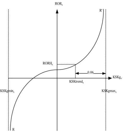
The normal rate of return to capital in branch s ( ROR )s is specified as an inverse logistic

function (see Figure 5) of the proportionate growth in sector’s s capital stock (Dixon and Rimmer, 2002):

s ,t s s s ,t s s s ,t

s s s s

ROR RORH ( 1 / B ) [ln( KSKg KSKg min ) ln( KSKg max KSKg )

ln( KSKtrend KSKg min ) ln( KSKg max KSKtrend )]

= + ⋅ − − − −

− + − (84)

where RORHs is the historically normal rate of return in branch s, KSKgs ,t is the capital

growth rate in industry s in year t, KSKg mins and KSKg maxs are the minimum and the

maximum possible growth rates of capital stock in branch s, KSKtrends is the industry’s

historically normal growth rate and Bs is a positive parameter. The minimum possible

growth rate is set at the negative of the rate of depreciation in branch s. This condition implies that investments in each branch of activity have positive values, such that once installed, capital cannot be shifted from one sector to another except for the gradual process of depreciation. The maximum possible growth rate of capital stock in industry s is set at KSKtrends plus lim INVs in order to avoid unrealistically large simulated growth rates

(Dixon and Rimmer, 2002). In the current version lim INVs is taken equal to 6 per cent for

all the branches. For example, if the historically normal growth rate in an industry is 4 per cent, the upper limit in any year t would not exceed 10 per cent.

Parameter ( B )s reflects the sensitivity of capital growth in branch s to variations in its

expected rate of return. It is derived by differentiating equation (84) with respect to

s ,t KSKg : s s s s s s s KSKg max KSKg min B SEA

( KSKg max KSKtrend ) ( KSKtrend KSKg min )

⎡ − ⎤ = _⋅⎢ _⎥ − ⋅ − ⎣ ⎦ (85) where: s ,t s ,t 1 ROR SEA KSKg − ⎛ ∂ ⎞ = ⎜_⎜ ⎟_⎟ ∂ ⎝ ⎠ (86)

(23)

s ,t s ,t s s ,t 1 ROR SEA KSKg KSKtrend KSKg − ⎛ ∂ ⎞ = ⎜_⎜ ₌ ⎟_⎟ ∂ ⎝ ⎠ (87)

where SEA is the reciprocal of the slope of the RR’ in Figure 5, which is considered to be

the same for all industries due to the lack of detailed estimates by branch.

The present value ( PVKs ,t) of investing a unit of capital in industry s in year t is defined as:

s ,t t s ,t 1 t 1 s t 1 s t

PVK = −PI +[ PK ₊ +PI₊ ⋅ +d PI₊ ⋅ −( 1 d )] /[ 1 NINT ]+ (88)

where PIt is the cost of buying a unit of capital (the price of composite investment good)

in year t, PKs ,t+PIt 1+ ⋅ds is the rental rate on industry’s s capital stock, ds is the

depreciation rate in branch s and NINTt is the nominal interest rate in year t (Dixon and

Rimmer, 2002). The purchase of one unit of capital in year t by industry s involves an immediate expenditure ( PI )t , followed by two benefits in year t+1 which are discounted

by ( 1+NINT )t : the rental value of an extra unit of capital in year t+1 ( PKs ,t 1+ +PIt 1+ ⋅d )s ,

including the depreciation, and the value at which the depreciated unit of capital can be sold in year t+1 [ PIt 1+ ⋅ −( 1 d )]s .

The expected rate of return on investment in industry s in year t is given by dividing both sides of (88) by PIt:

s ,t s ,t 1 t t 1 t t

ROR = − +1 [ PK ₊ / PI +PI₊ / PI ] /[ 1 NINT ]+ (89)

Under static expectations, investors are assumed to anticipate that the asset prices (the cost of buying a unit of capital) and the net rental rates will increase by the current rate of inflation ( RINF )t . Thus, the expected rate of return ( ROR )s ,t under static expectations is

given by:

s ,t s ,t t t t t t t

ROR = − +1 [ PK ⋅ +( 1 RINF ) / PI +PI ( 1 RINF ) / PI ] /[ 1⋅ + +NINT ] (90)

Simplifying further, we get:

s ,t s ,t t t

ROR = − +1 [ PK / PI +1] /( 1 RINT )+ (91)

where the real interest rate ( RINT )t is defined as:

t t t

(24)

RORs RORHs 0.06 KSKtrends KSKgs KSKgmaxs KSKgmins R R'

Figure 5. The expected rate of return for industry s

The weighted average real return to capital has been taken as a proxy for the real interest rate in AzorMod. The return to capital is expressed in real terms using the production price index:

t s ,t s ,t s ,t s ,t

s s

RINT [(PK=

∑

/ PD ) KSK⋅ ]/

∑

KSK (93)

The capital stock in industry s in the next period (year t+1) is given by:

s,t+1 s s,t s,t

KSK = (1 d ) KSK +INV− ⋅ (94)

where KSKs ,t is the current capital stock (in year t) and INVs ,t stand for the investments by

the branch s in year t.

The capital growth rate in terms of capital stock in year t+1 and the capital stock in year t is given by:

s ,t s ,t 1 s ,t

KSKg =KSK ₊ / KSK −1 (95)

whereas the actual growth rate of capital in industry s can be derived from equation. (84) as:

]

s ,t s ,t s s s s s s s ,t s s s s

KSKg ROR KSKg max ( KSKtrend KSKg min ) KSKg min ( KSKg max KSKtrend ) / ROR ( KSKtrend KSKg min ) ( KSKg max KSKtrend )

α α =_⎡⎣ ⋅ ⋅ − + ⋅ − _⎡⎣ ⋅ − + − (96)

(25)

s ,t s s s s s s s

{[(ROR RORH ) (KSKgmax KSKgmin )]/[(KSKgmax KSKtrend ) (KSKtrend KSKgmin )]} s ,t

ROR = e

α − ⋅ − − ⋅ − ₍₉₇₎

A first estimate of investments in the branch s in year t (INVS )s,t is derived from equations

(94)-(96) as:

s,t s,t s,t s s s s

s s s,t s s

s s s s,t

INVS = KSK [ ROR KSKgmax (KSKtrend KSKgmin )+ KSKgmin (KSKgmax KSKtrend )]/[ ROR (KSKtrend KSKgmin )+

(KSKgmax KSKtrend )]+d KSK α α ⋅ ⋅ ⋅ − ⋅ − ⋅ − − ⋅ (98)

while the actual level of investments in branch s in year t is provided by:

s,t s,t ss,t t c,t c,t t

ss c

INV = INVS /

∑

INVS ⋅(S −

∑

SV ⋅P )/PI (99)

which also insures the consistency between total investments and savings.

The model is solved dynamically with annual steps. The simulation horizon of the model has been set at 13 years but it can easily be extended.

2.13 Closure rules

The closure rules refer to the manner in which demand and supply of commodities, the macroeconomic identities and the factor markets are equilibrated ex-post. Due to the complexity of the model, a combination of closure rules is needed. The particular set of closure rules should also be consistent, to the largest extent possible, with the institutional structure of the economy and with the purpose of the model.

In mathematical terms, the model should consist of an equal number of independent equations and endogenous variables. The closure rules reflect the choice of the model builder of which variables are exogenous and which variables are endogenous, so as to achieve ex-post equality.

Three macro balances are usually identified in CGE models that can be a potential source of ex-ante disequilibria and must be reconciled ex-post (Adelman and Robinson, 1989):

The savings-investment balance; The government balance; The external balance.

The most widely used macro closure rule for CGE models is based on the investment and savings balance. In the model, the investment is assumed to adjust to the available domestic and foreign savings. This reflects an economy in which savings form a binding constraint.

Additional assumptions are needed with regard to regional government behaviour in AzorMod. First, regional government savings are fixed in real terms while regional government total current consumption adjusts to achieve the target set with respect to the government savings. The allocation between the consumption of different goods and services is provided by a Cobb-Douglas function. Secondly, the transfers received by the regional government from the Mainland government, from the EU, from the US and from the ROW are fixed in real terms. On the expenditure side, the regional government transfers to the households are also fixed in real terms.

For the external balance, the exchange rates are kept unchanged in the simulations, while the balances of the current accounts adjust. An alternative closure is also possible where

(26)

the balances of the current accounts corresponding to US and ROW are set while the real exchange rates adjust.

The setup of the closure rules is important in determining the mechanisms governing the model. Therefore, the closure rules should be established also taking into account the policy scenario in question.

According to Walras’ law if (n-1) markets are cleared the nth one is cleared as well. Therefore, in order to avoid over-determination of the model, the current account balance with respect to ROW has been dropped (see equation (61), section 2.6). However, the system of equations guarantees, through Walras’ law, that the total imports from ROW less the total exports to ROW and the transfers from ROW equals the current account balance.

(27)

2.14 Model equations 2.14.1 Firms s s s SF = shYKF⋅

∑

PK ⋅KSK (A.1) s s s KL = aKL ⋅XD _(A.2) s s s F F ( F 1) s s s s s s s s KSK = KL {PKL /[PK (1+tk )+d⋅ ⋅ ⋅PI]}σ ⋅γFKσ ⋅aF σ − _(A.3) s s s F F ( F 1) s s s s s s s s LSK = KL { PKL /[PL (1+premLSK ) (1+tl /(1 tl ))]}⋅ ⋅ ⋅ − σ ⋅γFLσ ⋅aF σ − (A.4) s s s s s s s s s s

PKL KL = PK (1+tk ) KSK +PL (1+premLSK ) (1+tl /(1 tl )) LSK +DEP PI⋅ ⋅ ⋅ ⋅ ⋅ − ⋅ ⋅ (A.5)

s s s s s s

s s s s s

c,s s c,s c ctm,c,s ctm c,s

c ctm

PD (1 tp +tsp +tspeuea MUtspeu+tspeufi MUtspeu+tspeuer MUtspeu+tspeues MUtspeu+tspusa ) XD = PKL KL

{io XD [ (1 tsic ) P + tcictm P ] (1+vatic )}

⋅ − ⋅ ⋅ ⋅ ⋅ ⋅ ⋅ + ⋅ ⋅ − ⋅ ⋅ ⋅

∑

(A.6) 2.14.2 Households

c ctm,c,qu ctm c,qu c,qu c,qu c,qu c ctm,c,qu ctm

ctm ctm

c,qu c,qu c,qu c,qu c,qu qu cc ctm,cc,qu ctm cc ctm

cc,qu

[P + tchtm P ] (1+texc ) (1+tc +vatc ) C = [P + tchtm P ]

(1+texc ) (1+tc +vatc ) H H {CBUD [P + tchtm P ]

(1+texc ) ( µ α ⋅ ⋅ ⋅ ⋅ ⋅ ⋅ ⋅ ⋅ + ⋅ − ⋅ ⋅ ⋅

∑

cc,qu cc,qu cc,qu 1+tc +vatc )⋅µH }

(A.7)

qu qu s s qu s s qu

s s

qu qu

YH = shYKH PK KSK +shYLH PL ( 1+premLSK ) LSK TRHML ERML+shUNEMPB trep PL UNEMP+TRHG PCINDEX

⋅ ⋅ ⋅ ⋅ ⋅ + ⋅ ⋅ ⋅ ⋅ ⋅

∑

(A.8) qu qu qu qu CBUD = (1 ty ) YH− ⋅ −SH _(A.9) qu qu qu qu SH = MPS ⋅ −(1 ty ) YH⋅ _(A.10) qu elasS qu qu qu qu

MPS = MPSZ ⋅{[ (1 ty− ) PKavr]/[(1 tyz⋅ − ) PKavrZ]}⋅

(A.11)

2.14.3 Regional government

GREV = TRPROP+TRPROD+TRANSR _(A.12)

qu qu s s s qu s TRPROP =

∑

ty ⋅YH +

∑

tk ⋅KSK ⋅PK (A.13) s s s c ctm,c,qu ctm c,qu s c ,qu ctm

c,qu c,qu c,qu c,qu c ctm,c ctm c c c ctm

c,s c ctm,c,s ctm c,s c,s s ctm

TRPROD = tp XD PD {[P + tchtm P ] [ texc ( 1 texc ) ( tc +vatc )] C } [P + tcitm P ] vati I

[(1 tsic ) P + tcictm P ] vatic io XD

⋅ ⋅ + ⋅ ⋅ + + ⋅ ⋅ + ⋅ ⋅ ⋅ + − ⋅ ⋅ ⋅ ⋅ ⋅

∑

c c c ,s c c c c c c (tmus PWMUS MUS ERUS)+ (tmrw PWMROW MROW ERROW)