Development of prognostic aerosol–cloud interactions combining a chemistry transport model and a regional climate model

(1)

GMDD

8, 897–933, 2015

Development of coupled model setup

M. A. Thomas et al.

Title Page

Abstract Introduction

Conclusions References

Tables Figures

◭ ◮

Back Close

Full Screen / Esc

Printer-friendly Version Interactive Discussion

Discussion

P

a

per

|

Discussion

P

a

per

|

Discussion

P

a

per

|

Discussion

P

a

per

|

Geosci. Model Dev. Discuss., 8, 897–933, 2015 www.geosci-model-dev-discuss.net/8/897/2015/ doi:10.5194/gmdd-8-897-2015

This discussion paper is/has been under review for the journal Geoscientific Model Development (GMD). Please refer to the corresponding final paper in GMD if available.

Development of prognostic aerosol–cloud

interactions combining a chemistry

transport model and a regional climate

model

M. A. Thomas1, M. Kahnert1,2, C. Andersson1, H. Kokkola3, U. Hansson1, C. Jones1,4, J. Langner1, and A. Devasthale1

1

Research Department, Swedish Meteorological and Hydrological Institute, Folkborgsvägen 17, 60176 Norrköping, Sweden

2

Department of Earth and Space Sciences, Chalmers University of Technology, 41296 Gothenburg, Sweden

3

Finnish Meteorological Institute, Kuopio, Finland

4

National Centre for Atmospheric Science, School of Earth and Environment, University of Leeds, LS2 9JT Leeds, UK

Received: 25 November 2014 – Accepted: 21 January 2015 – Published: 3 February 2015 Correspondence to: M. A. Thomas (manu.thomas@smhi.se)

(2)

GMDD

8, 897–933, 2015

M. A. Thomas et al.

Title Page

Tables Figures

◭ ◮

Back Close

Full Screen / Esc

Discussion

P

a

per

|

Discussion

P

a

per

|

Discussion

P

a

per

|

Discussion

P

a

per

|

Abstract

To reduce uncertainties and hence, to obtain a better estimate of aerosol (direct and indirect) radiative forcing, next generation climate models aim for a tighter coupling between chemistry transport models and regional climate models and a better rep-resentation of aerosol–cloud interactions. In this study, this coupling is done by first

5

forcing the Rossby Center regional climate model, RCA4 by ERA-Interim lateral bound-aries (LBCs) and SST using the standard CDNC (cloud droplet number concentration) formulation (hereafter, referred to as the “stand-alone RCA4 version” or “CTRL” sim-ulation). In this simulation, the CDNCs are assigned fixed numbers based on if the underlying surface is land or oceanic. The meteorology from this simulation is then

10

used to drive the chemistry transport model, MATCH which is coupled online with the aerosol dynamics model, SALSA. CDNC fields obtained from MATCH-SALSA are then fed back into a new RCA4 simulation. In this new simulation (referred to as “MOD” simulation), all parameters remain the same as in the first run except for the CDNCs provided by MATCH-SALSA. Simulations are carried out with this model set up for the

15

period 2005–2012 over Europe and the differences in cloud microphysical properties and radiative fluxes as a result of local CDNC changes and possible model responses are analyzed.

Our study shows substantial improvements in the cloud microphysical properties with the input of the MATCH-SALSA derived 3-D CDNCs compared to the stand-alone

20

RCA4 version. This model set up improves the spatial, seasonal and vertical distribu-tion of CDNCs with higher concentradistribu-tion observed over central Europe during summer half of the year and over Eastern Europe and Russia during the winter half of the year. Realistic cloud droplet radii (CD radii) values have been simulated with the maxima reaching 13 µm whereas in the stand-alone version, the values reached only 5 µm.

25

(3)

GMDD

8, 897–933, 2015

M. A. Thomas et al.

Title Page

Tables Figures

◭ ◮

Back Close

Full Screen / Esc

Discussion

P

a

per

|

Discussion

P

a

per

|

Discussion

P

a

per

|

Discussion

P

a

per

|

those obtained using the stand-alone RCA4 version. These changes resulted in a sig-nificant decrease in the total annual mean net fluxes at the top of the atmosphere (TOA) by−5 W m−2over the domain selected in the study. The TOA net fluxes from the “MOD” simulation show a better agreement with the retrievals from CERES instrument. The aerosol indirect e_ffects are evaluated based on 1900 emissions. Our simulations

es-5

timated the domain averaged annual mean total radiative forcing of−0.64 W m−2with larger contribution from the first indirect aerosol effect than from the second indirect aerosol e_ffect.

1 Introduction

The scientific understanding of the climate effects of the different aerosol species as

10

well as their representation in models and their physical and chemical transformation under different meteorological conditions is still low (Boucher et al., 2013). Aerosols have a direct radiative effect by scattering and absorbing short and long wave radia-tion, thereby changing the reflectivity, transmissivity and absorbtivity of the atmosphere. They can further act as cloud condensation nuclei (CCN), thereby influencing the

mi-15

crophysical properties of clouds. This, in turn, can impact the optical properties and lifetimes of clouds, thus, indirectly a_ffecting the radiative properties of the atmosphere (Penner et al., 2004). Apart from ambient conditions, the ability of the aerosols to act as CCN depends on the size distribution (Dusek et al., 2006) and, for particles in the size range between 40 and 200 nm, on the chemical composition and mixing state

20

(McFiggans et al., 2006).

The direct effect of aerosols and even more so, their indirect impact on radiative forcing have been identified as the largest sources of uncertainty in quantifying the radiative energy budget and its impact on climate system (Forster et al., 2007). The study of these effects accurately and in great detail requires coupling of atmospheric

25

(4)

GMDD

8, 897–933, 2015

M. A. Thomas et al.

Title Page

Tables Figures

◭ ◮

Back Close

Full Screen / Esc

Discussion

P

a

per

|

Discussion

P

a

per

|

Discussion

P

a

per

|

Discussion

P

a

per

|

the recent generation of models use the regional climate models at a higher horizontal and vertical resolution instead of GCMs (for example, WRF-Chem (Grell et al., 2005), ENVIRO-HIRLAM (Baklanov et al., 2008), RegCM3-CAMx (Huszar et al., 2012; Qian and Giorgi, 1999; Qian et al., 2001 etc.). Recently, Baklanov et al. (2014) summarized the status of the online/o_ffline European coupled meteorology and chemistry transport

5

models with varying degrees of complexity in the representation of dynamical and phys-ical processes, aerosol–cloud-climate interactions, radiation schemes etc. The main conclusion was that an online integrated modeling approach is the future and can be adapted to several modeling communities such as climate modeling and air quality re-lated studies (Baklanov et al., 2014 and the references therein). The study also showed

10

that for climate modeling, the inclusion of feedback processes is the most important and significant improvements were noticeable in climate-chemistry/aerosols interac-tions. Whether the coupling need to be online or offline depends on the specific study. For example, Folberth et al. (2011) showed that in long-lived greenhouse gas forcing experiments, the online approach did not give significant improvements, whereas, for

15

short-lived climate forcers, aerosols in particular, online approach is very beneficial. Here, we attempt a similar approach by adapting the Rossby Center regional climate model, RCA4 for the o_ffline ingestion of CDNCs from the cloud activation module em-bedded in the chemistry transport model, MATCH that is online coupled to the aerosol dynamics model, SALSA. Such a coupling is unique in many ways:

20

1. A more detailed description of the emissions, transport, particle growth, deposi-tion, aerosol processes can be included so as to obtain an accurate evaluation of aerosol radiative effects on a higher spatial resolution compared to global models (Colarco et al., 2010),

2. it is possible to assess the level of detail that is required to describe the effects on

25

a regional scale and

(5)

GMDD

8, 897–933, 2015

M. A. Thomas et al.

Title Page

Tables Figures

◭ ◮

Back Close

Full Screen / Esc

Discussion

P

a

per

|

Discussion

P

a

per

|

Discussion

P

a

per

|

Discussion

P

a

per

|

In this paper, we present the results from a full fledged working version of the cou-pling between a chemistry transport model (CTM) with a detailed aerosol dynamics model and a regional climate model. The coupling between these two model systems are offline and is done through CDNCs calculated by the CTM. The drawback of of-fline coupling is that there is no feedback on the simulation of chemistry and aerosols

5

from changes in meteorology due to altered CDNC/radiation and no coupling to SST. In the following subsections, we introduce the models used in this study, their coupling and the improvements made in the cloud microphysical properties and radiative forcing through this coupling.

2 Models used and experimental setups

10

2.1 Models used

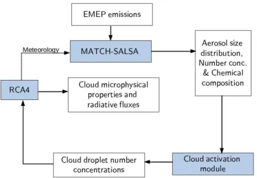
The schematic of the model coupling is shown in Fig. 1. In this study, we use the Multiple-scale Atmospheric Transport and Chemistry (MATCH) model (Robertson et al., 1999; Andersson et al., 2007) which is a Eulerian CTM that accounts for trans-port, chemical transformation and deposition of chemical tracers in the atmosphere

15

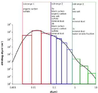
based on EMEP emissions (http://www.ceip.at). The MATCH model is online coupled to the aerosol dynamics model, SALSA (Kokkola et al., 2008) that takes into account physical processes such as nucleation of particles, growth of particles by condensa-tion and coagulacondensa-tion and computes the size distribucondensa-tion, number concentracondensa-tion and chemical composition of the aerosol species. A sectional representation of the aerosol

20

size distribution is considered and has three main size regimes ((a) 3–50 nm, (b) 50– 700 nm and (c)>700 nm) and each regime is again subdivided into smaller bins and into soluble and insoluble bins adding up to a total of 20 bins. A schematic of the sectional size distribution and the aerosol species considered in each bin is shown in Fig. 2. Anthropogenic precursor emissions such as primary particulate matter (PM),

25

(6)

GMDD

8, 897–933, 2015

M. A. Thomas et al.

Title Page

Tables Figures

◭ ◮

Back Close

Full Screen / Esc

Discussion

P

a

per

|

Discussion

P

a

per

|

Discussion

P

a

per

|

Discussion

P

a

per

|

EMEP expert emissions inventory. Primary PM is divided into EC, OC and other emis-sions. Isoprene emissions are modeled online depending on the meteorology based on the methodology by Simpson et al. (1995). The terpene emissions (α-piniene) is taken from the modeled fields by the EMEP model. Sea salt is parameterized following the scheme of Foltescu et al. (2005), but, modified for varying particle sizes. This means

5

that Mårtensson et al. (2003) is used if the particle diameter is≤1 µm and Monahan et al. (1986) is used otherwise.

The coupling of MATCH with SALSA and the evaluation of this model set up is de-scribed in detail in Andersson et al. (2014). A cloud activation model that computes 3-D CDNCs based on the prognostic parameterization scheme of Abdul-Razzak and Ghan

10

(2002) specifically designed for sectional representation of bins is embedded in the MATCH-SALSA model. In addition to the updraft velocity and supersaturation of the air parcel, this scheme simulates the efficiency of the an aerosol particle to be converted to a cloud droplet depending on the number concentration and chemical composition of the particles. The updraft velocity is computed as the sum of the grid mean vertical

15

velocity and turbulent kinetic energy (TKE) for stratiform clouds (Lohmann et al., 1999) derived from the RCA4 simulation. These CDNCs are then o_ffline coupled to a regional climate model, RCA4 (Samuelsson et al., 2011) that provide us information on the cloud microphysical properties such as cloud droplet radii, cloud liquid water path as well as radiative fluxes. In the stand-alone version of RCA4, the total number of cloud

20

particles were assigned fixed numbers over the whole domain based on whether the surface is oceanic (150 cm−3) or land (400 cm−3) and scaled vertically. These are fur-ther used in calculation of e_ffective radius of cloud droplets and in the autoconversion process (conversion of cloud droplet to rain). These are now replaced by the 3-D CDNC fields obtained from the cloud activation model.

25

2.2 Experimental setup – 1

(7)

GMDD

8, 897–933, 2015

M. A. Thomas et al.

Title Page

Tables Figures

◭ ◮

Back Close

Full Screen / Esc

Discussion

P

a

per

|

Discussion

P

a

per

|

Discussion

P

a

per

|

Discussion

P

a

per

|

along with fields necessary to compute the updraft velocity are used to drive MATCH-SALSA-cloud activation model. The aerosol properties are used in the cloud activation model to derive the 6 hourly CDNCs which are then employed to re-run RCA4 with dynamic rather than prescribed CDNCs to obtain cloud microphysical properties and radiative e_ffects. Simulations were carried out with this model set up at 44 km×44 km

5

spatial resolution for the European domain and 24 levels in the vertical (up to 200 hPa) for an 8 year period (2005–2012). Here, we look into the improvements in the cloud microphysical properties and radiative fluxes with the incorporation of dynamic CDNCs where in only local land surface fluxes can respond to these changes, hereby referred to as the MOD simulation. These results are compared with the control simulation,

10

hereby referred to as the CTRL simulation in which the stand-alone version of RCA4 is used.

2.3 Experimental setup – 2

To evaluate the indirect aerosol effects due to the present day anthropogenic aerosols, the pre-industrial (PI) emissions required for this simulation were taken from those

de-15

veloped for the ECLAIRE project (Effects of climate change on air pollution impacts and response strategies) for the year 1900 (http://www.eclaire-fp7.eu). The PI anthro-pogenic precursor emissions were provided for CO, NH₃, NO_x, SO_x and VOC. The physiography files and the other emissions (biogenic emissions, DMS and volcanic) are kept the same as in the original model setup. The particulate organic matter

emis-20

sions are reduced to 14 % of the current emission levels in the pre-industrial set up based on the study by Carslaw et al. (2013). Simulations were carried out at the same spatial resolution as in the previous setup and for the same European domain and for the same meteorology from 2005–2012. Here, we address the changes in cloud prop-erties with respect to the emissions from the PI period without the climate feedbacks

25

(8)

GMDD

8, 897–933, 2015

M. A. Thomas et al.

Title Page

Tables Figures

◭ ◮

Back Close

Full Screen / Esc

Discussion

P

a

per

|

Discussion

P

a

per

|

Discussion

P

a

per

|

Discussion

P

a

per

|

3 Model evaluation and results

3.1 Aerosol number concentrations

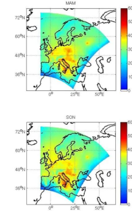
Figure 3 shows the spatial distribution of the seasonal mean accumulation mode aerosol number concentrations from MATCH-SALSA model simulations driven by RCA4 meteorology. The main contribution to accumulation mode particles are from

5

SO42−, EC, OC, sea salt and mineral dust. In the figure, emphasis is given to accumu-lation mode particles as they can act as CCN and, depending on the water availability and updraft velocity be efficiently converted into cloud droplets. A clear seasonality is noticeable with highest concentrations during the summer months and lowest during the winter months. Concentrations reach as high as 600 cm−3over southern European

10

subcontinent during summer. This may be partly due to relatively large emissions of primary fine particles and gaseous SO_x, and partly due to less precipitation in south-ern Europe compared to the rest of Europe resulting in longer residence times of these particles in the atmosphere (Andersson et al., 2014).

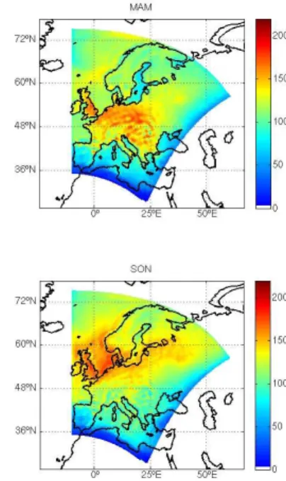
3.2 Cloud droplet number concentrations

15

The seasonal mean in-cloud averaged CDNCs for the European domain is presented in Fig. 4. During the summer half of the year, CDNCs are extremely high, reaching as high as 225 cm−3over central Europe mainly because of summer time vertical mixing, high probability of liquid clouds and is also, consistent with high aerosol number con-centrations simulated during this time. The land–sea contrast is more prominent during

20

the summer months compared to the other seasons. A closer comparison with Fig. 3 reveals that regions of high CDNCs correspond mostly with regions of high accumu-lation mode aerosol particles. However, in some regions, this correaccumu-lation is not very noticeable, especially over the Mediterranean in summer. This may be due to subsi-dence and lack of cloud in these regions. Higher CDNCs are observed in the Eastern

(9)

GMDD

8, 897–933, 2015

M. A. Thomas et al.

Title Page

Tables Figures

◭ ◮

Back Close

Full Screen / Esc

Discussion

P

a

per

|

Discussion

P

a

per

|

Discussion

P

a

per

|

Discussion

P

a

per

|

Europe and Russia can be mainly attributed to the increased residential biomass burn-ing durburn-ing the autumn and winter months (Yttri et al., 2014).

Storelvmo et al. (2009) showed that di_fferences in the cloud droplet activation would account for about 65 % of the total spread in shortwave forcing. So, it is important to see if this model setup reproduces the spatial distribution of CDNCs realistically.

5

The high droplet concentrations simulated over land compared to oceans agrees well with the previous studies of Barahona et al. (2011) and Moore et al. (2013). Zeng et al. (2014) analyzed the CDNCs from MODIS and CALIOP sensors and it is evident that the droplet concentrations over European subcontinent would be on an average between 150–200 cm−3and over oceans, the concentrations are as low as 100 cm−3.

10

This agrees well with our simulations.

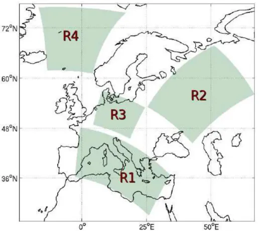
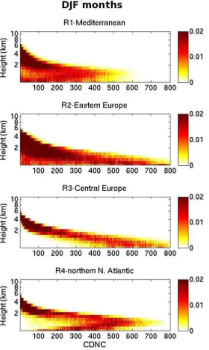
To understand the vertical distribution of CDNCs, we select the following 4 regions as in Fig. 5 – R1: Mediterranean R2: Eastern Europe R3: Central Europe and R4: northern N. Atlantic. Figure 6 shows the joint histograms of CDNC and height (in km) over the four selected regions for winter (DJF) and summer (JJA) months respectively.

15

It can be seen that the majority of the CDNC values are less than 500 cm−3, but occa-sionally values also reach as high as 800 cm−3irrespective of season and region. The figures also show an interesting seasonality of the PDFs (probability distribution func-tions) of CDNC. For example over the Mediterranean (R1), two peaks can be observed in summer, one around 3 km and another in the boundary layer, however, in winter,

20

only one peak is present and is located below 2 km. This is mainly due to the stronger vertical mixing of aerosols together with increased buoyancy and convection in sum-mer. It is well known that the frequency of occurrence of very low level water clouds is high over this region during summer, while, in winter, the baroclinic disturbances lead to northward transport of winter storms over this region. Over Eastern Europe

25

(10)

GMDD

8, 897–933, 2015

M. A. Thomas et al.

Title Page

Tables Figures

◭ ◮

Back Close

Full Screen / Esc

Discussion

P

a

per

|

Discussion

P

a

per

|

Discussion

P

a

per

|

Discussion

P

a

per

|

seasons. The opposite is observed over northern N. Atlantic (R4) with maxima CDNC simulated at around 1.5 km in winter and in the boundary layer in summer. This can be attributed to the long range of transport of pollutants from across the Atlantic observed during the winter months (HTAP, 2010).

3.3 Cloud droplet radii

5

As mentioned in Sect. 2, both the CTRL and MOD simulations follows the same pa-rameterization scheme of Wyser et al. (1999) in the radiation and is formulated as in Eq. (1). The effective radius for spherical droplets is estimated as,

r_e,water₌ 3CC

4πρ_lkN (1)

where CC is the cloud condensate content in kg m−3,ρ_lis the density of liquid water,N 10

is the number concentration of cloud droplets in m−3,kis a constant depending on ma-rine or continental clouds. In the CTRL simulation,Nwas assigned 150 and 400 cm−3 depending on the underlying surface, however, in the MOD simulation dynamic CDNCs are used.

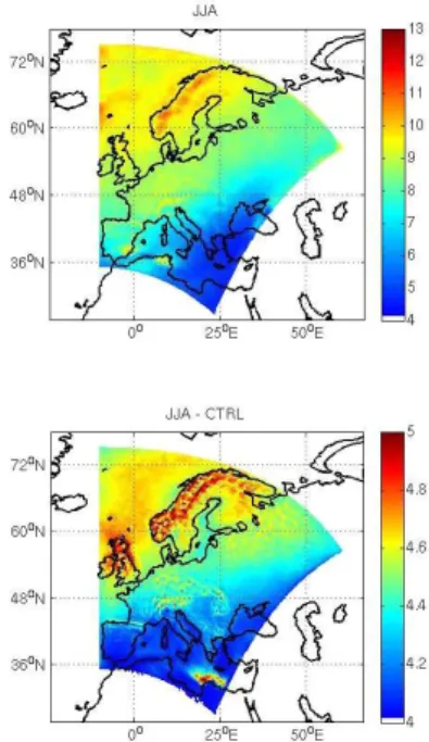
The winter and summer mean cloud droplet radii in liquid water clouds for the MOD

15

simulation (top row) and the CTRL simulation (2nd row) is discussed in Fig. 7. At a first glance, apart from the spatial di_fferences, one notice the strong disparity in the range of the radii values. In the MOD simulation, CD radii reach as high as 13 µm, whereas in the CTRL simulation, the maxima observed is 5 µm. It can be seen that the radii of the droplets are much lower in the summer months compared to the winter months

20

basically due to the increased pollution during summer resulting in smaller droplets. In Fig. 8, the joint histograms of CD radii and height during the summer over Mediter-ranean and Eastern Europe in MOD simulation are shown. The corresponding pattern in the CTRL simulation is shown as the solid line. It can be seen that the CTRL sim-ulation does not exhibit any variability. However, the MOD simsim-ulation shows a distinct

(11)

GMDD

8, 897–933, 2015

M. A. Thomas et al.

Title Page

Tables Figures

◭ ◮

Back Close

Full Screen / Esc

Discussion

P

a

per

|

Discussion

P

a

per

|

Discussion

P

a

per

|

Discussion

P

a

per

|

variability in height and range. It can be seen that over the Mediterranean and over Eastern Europe, a wide range of droplet radii can be observed from as low as 5 µm up to 16 µm and the larger droplets are present at around 2.0–4.0 km s. However, there is a higher probability of observing larger droplets over Eastern Europe compared to the Mediterranean.

5

The critical droplet radius at which large scale precipitation occurs is set to 10 µm in the microphysics scheme. This would mean that with these low CD radii values obtained in the stand-alone RCA4 model, precipitation would be absent. It is important to note that the plotted CD radii values are derived from the model radiation scheme (ie. this is the radiatively active CD radii). For more details, refer Appendix A.

10

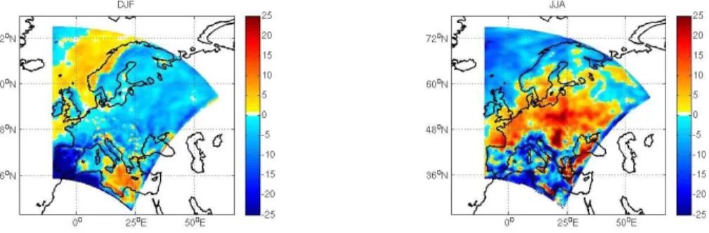
3.4 Cloud liquid water path

Figure 9 refers to the percentage change in column integrated cloud water (CLWP) in the MOD simulations compared to CTRL simulations averaged over the winter (DJF) and summer (JJA) months. Positive values mean that the CLWP increased in the MOD simulations compared to the CTRL and vice versa. It can be seen that during the winter

15

months, there is a significant decrease (up to 25 %) in the vertically integrated cloud liquid water over land and a slight increase over the water bodies when the 3-D CD-NCs are used. However, during the summer months, the pattern is reversed with a no-ticeable increase in CLWP over most of the European subcontinent. The decrease in CLWP with increase in CD radii is consistent and may be partly attributed to

precipita-20

tion removal. In the model, the critical droplet radius at which autoconversion becomes e_fficient is set to 10 µm. When the CD e_ffective radius exceeds this critical droplet ra-dius, precipitation occurs. However, over land during summer, an increase in CLWP is observed and can be partly due to the fact that the increase in CD radius is not su_fficient to trigger precipitation.

25

(12)

ef-GMDD

8, 897–933, 2015

M. A. Thomas et al.

Title Page

Tables Figures

◭ ◮

Back Close

Full Screen / Esc

Discussion

P

a

per

|

Discussion

P

a

per

|

Discussion

P

a

per

|

Discussion

P

a

per

|

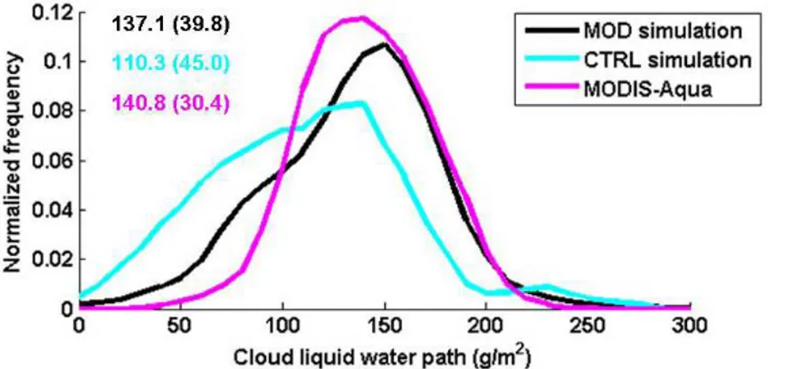
fects which are the main application focus of the coupling attempted here. We used a decade long data record (2003–2012) from the Moderate Resolution Imaging Spec-troradiometer (MODIS) sensor flying onboard NASA’s Aqua satellite since 2002 (Plat-nick et al., 2003; Hubanks et al., 2008). The monthly Level 3 data from the Collection 5 are analysed over the study area to compute probability density function of LWP for the

5

boreal summer months of JJA (June, July and August), when liquid clouds are most prevalent and the quality of satellite retrievals is also best. The comparison is shown in Fig. 10. We observe substantial improvement in the distribution of LWP in the MOD simulation compared to the CTRL-Simulation. The inclusion of the chemistry-aerosol– cloud microphysical link leads to more realistic distribution of LWP that is closer to the

10

observations. At the lower end of the distribution, the model still slightly overestimates the frequency of those optically thin liquid water clouds. But the LWP of optically thick clouds, which are most abundant and play a key role in the radiation budget over the study area, shows substantial improvements in the MOD simulation.

3.5 Total radiative fluxes at the TOA

15

The difference in the annual mean total net fluxes at the TOA due to these changes in the cloud microphysical properties is shown in Fig. 11. A significant change is seen over most of the domain with decreases up to−5 W m−2when the CDNC values are assigned fixed numbers depending on the underlying surface.

To evaluate the TOA radiative fluxes, we used a decade long data for comparison

20

from the Clouds and the Earth’s Radiant Energy System (CERES) sensor that is flying onboard Aqua satellite as well (Wielicki et al., 1996) (more information is available at http://ceres.larc.nasa.gov/documents/DQ_summaries/CERES_EBAF_Ed2.8_DQS. pdf). The Level 3 Energy Balanced and Filled estimates of all-sky net top of the at-mosphere fluxes (EBAF-TOA, Edition 2.8) are analysed for comparison with MOD and

25

(13)

GMDD

8, 897–933, 2015

M. A. Thomas et al.

Title Page

Tables Figures

◭ ◮

Back Close

Full Screen / Esc

Discussion

P

a

per

|

Discussion

P

a

per

|

Discussion

P

a

per

|

Discussion

P

a

per

|

4 Aerosol radiative forcing at the top of the atmosphere

In this section, we evaluate the e_ffect of changing cloud albedo and cloud lifetime due to the present day anthropogenic aerosols which is widely known as the first indirect aerosol e_ffect (Twomey, 1959) and the second indirect aerosol e_ffect (Albrecht, 1989) respectively. In a review paper, Lohmann and Feichter (2005) summarized the aerosol

5

radiative effects into positive and negative perturbations to the radiation budget. Both the indirect aerosol effects tend to cool the Earth system by increasing the cloud optical depth and cloud cover, thereby resulting in the reduction of the net radiation reaching the TOA and surface.

The local radiative forcing associated with these IAE are in most cases estimated

10

as the di_fference between the perturbed and unperturbed radiative fluxes. The per-turbed case is the current climate scenario and in the unperper-turbed case, the fluxes are calculated based on a pre-industrial or pristine scenario with meteorology and SST remaining the same in the both cases. In this study, for the unperturbed case (PI), we use the pre-industrial emissions from 1900s as explained in Sect. 2.3. And the present

15

day climate scenario as in the “MOD” simulations would be our perturbed case (PD). In the following paragraphs, we analyze the changes in CDNC and CLWP in the (PD-PI) case and the TOA aerosol radiative forcing over Europe which arises mainly due to the response of the land surface without other climate feedbacks. Figures 13–15 show the annual mean di_fference in aerosol number concentrations, CDNC and CLWP

20

respectively with respect to the PI emissions expressed as a percentage.

It can be seen that there is approximately 50–80 % increase in the aerosol number concentrations with respect to PI era over southern and Eastern European subcon-tinent and around 10–30 % over the rest of Europe and over the oceans. The steep increase in the aerosol concentrations may be attributed to the increase in

anthro-25

(14)

GMDD

8, 897–933, 2015

M. A. Thomas et al.

Title Page

Tables Figures

◭ ◮

Back Close

Full Screen / Esc

Discussion

P

a

per

|

Discussion

P

a

per

|

Discussion

P

a

per

|

Discussion

P

a

per

|

the spatial distribution of the annual mean indirect aerosol forcing when using the 1900 reference value over the study region. The European domain averaged annual mean radiative forcing is−0.64 W m−2, with values reaching as high as−1.3 W m−2. This is comparable to the estimate of−0.96 W m−2 obtained by Carslaw et al. (2013) for the global mean forcing using the same reference period.

5

We also estimated the individual contribution of the first and second IAE to the total aerosol radiative forcing. This is done by turning offthe individual IAEs by prescribing the fixed values for CDNCs as in the stand-alone RCA4 version in the radiation and cloud microphysics calculation (Lohmann and Feichter, 2001).

In IPCC-2013 (Boucher et al., 2013) it was pointed out that the estimated values of

10

the first IAE constitute the largest uncertainty and vary significantly between the di_ff er-ent models. The impact of changes of aerosols on cloud albedo through the changes in droplet radius (first IAE) is estimated from our model set up to be−0.57 W m−2when averaged over the European domain. IPCC models estimated the global annual mean first IAE to be−0.7 W m−2and can vary widely from−1.8 to−0.3 W m−2. However, the

15

impact of changes of aerosols on cloud lifetime via the modification of precipitation effi -ciency is estimated to be−0.14 W m−2when averaged over the European domain used in this study. Studies have shown that the uncertainties in this are even larger compared to the first IAE. Depending on the autoconversion schemes used in the global models, Rotstayn and Liu (2005) showed that the global mean second IAE can vary from−0.71

20

to−0.28 W m−2, of which the scheme used to obtain the value of−0.28 W m−2is more realistic.

5 Conclusions

In this study, we coupled the Rossby Center regional climate model, RCA4 for the of-fline ingestion of CDNCs from the cloud activation module that is embedded in the

25

(15)

rep-GMDD

8, 897–933, 2015

M. A. Thomas et al.

Title Page

Tables Figures

◭ ◮

Back Close

Full Screen / Esc

Discussion

P

a

per

|

Discussion

P

a

per

|

Discussion

P

a

per

|

Discussion

P

a

per

|

resentation of emissions, transport, particle growth, deposition, aerosol processes can be included at a higher resolution compared to global models. Simulations were carried out with this set up for the period 2005–2012 over Europe using present day emissions (PD) from EMEP for the year 2000 and also, using the stand-alone version of RCA4. We carried out two sets of analysis:

5

1. Investigate the improvements in the cloud microphysical properties with the input of the 3-D CDNCs that replaced the assigned fixed numbers in the stand alone version of RCA4 based on if the underlying surface warm-continental or cold-oceanic.

2. Evaluate the indirect aerosol effects using this integrated modeling approach

us-10

ing the PI emissions taken from the ECLAIRE project. The particulate matter in the PI period are reduced to 14 % of the current levels based on Carslaw et al. (2013).

This model set up improves the spatial, seasonal and vertical distribution of CDNCs with higher concentration observed over central Europe during summer half of the year

15

and over Eastern Europe and Russia during the winter half of the year. Realistic cloud droplet radii numbers has been simulated with the maxima reaching 13 µm whereas in the stand-alone version, the values reached only 5 µm. The stand-alone version of RCA4 over-estimated the vertically integrated cloud water by up to 25 % in winter and underestimated by similar magnitude in summer over the European subcontinent.

20

Comparisons with satellite retrievals from MODIS reveals a significant improvement in the LWP distribution; the median and SD values obtained from the MOD simulation is much closer to observations than the CTRL simulation. A significant decrease by up to−5 W m−2in the total TOA net fluxes is simulated owing to these changes. The TOA net fluxes obtained with the new model setup show a better agreement with net flux

25

(16)

GMDD

8, 897–933, 2015

M. A. Thomas et al.

Title Page

Tables Figures

◭ ◮

Back Close

Full Screen / Esc

Discussion

P

a

per

|

Discussion

P

a

per

|

Discussion

P

a

per

|

Discussion

P

a

per

|

Using the pre-industrial emissions from 1900s, we estimated an increase of around 50–70 % CDNCs over southern and Eastern Europe and below 30 % over the rest of Europe in the present day climate consistent with the increases in aerosol number concentrations and correspondingly, an increase in CLWP is simulated over our study area. These changes resulted in an annual mean TOA radiative forcing over Europe

5

of−0.64 W m−2which is comparable to previous estimates for the same reference pe-riod. It was also estimated that the contribution from the first IAE is larger than the contribution from the second IAE.

Appendix A

In a given timestep,t₌n, the thermodynamic tendencies resulting from resolved

dy-10

namics and parameterized vertical turbulent fluxes are first calculated. These terms are stored in the relevant tendency terms, ∂χ_∂t att₌n. Next, the radiation scheme is called using the thermodynamic values (temperature,T; humidity,q; cloud water, cw etc.) valid att₌n. After the radiation fluxes have been calculated, the model calls the surface scheme, then, convection and finally, condensation and cloud microphysics is

15

called. On entering the microphysics scheme, the thermodynamic variables valid at

t₌nare updated by the tendencies from dynamics and turbulence. For example,

T₌T_n_{+ ∆}t×

_∂T

∂t|dyn+ ∂T

∂t|turb

and these variables are used to calculate a new value of cw,q etc. consistent with the updated saturated state of the atmosphere. With this, calculated cloud water can

in-20

crease locally due to the dynamical and turbulent terms and this re-calculated CD radii for the autoconversion process in the microphysics scheme may be substantially larger than in the radiation scheme (exceeding the threshold for precipitation onset of 10 µm). With the microphysics scheme, precipitation removal of generated cloud water is also parameterized, hence, the fraction of the newly generated cloud water is removed as

(17)

GMDD

8, 897–933, 2015

M. A. Thomas et al.

Title Page

Tables Figures

◭ ◮

Back Close

Full Screen / Esc

Discussion

P

a

per

|

Discussion

P

a

per

|

Discussion

P

a

per

|

Discussion

P

a

per

|

rain. The resulting cw tendency due to condensation and subsequent precipitation re-moval is then incremented on tot₌nvalues, along with all other tendencies fromt₌n

to give new values for the next timestep. In this manner, CD radii in the microphysics scheme can increase above the threshold for onset of precipitation and then, as a result of this precipitation removal of cloud water decrease again below the threshold. The

5

low (precipitation a_ffected) value of cloud water is what the radiation scheme “sees” in each timestep leading to a low estimate in CD radii.

Code availability

The di_fferent model source codes and the coupled system used in this study are not entirely available for open source distribution at present, but can be made available to

10

interested users/investigators upon request. The aerosol microphysics code, SALSA is distributed under Apache 2.0 license, while the regional climate model RCA4 and the chemistry transport model MATCH are available upon request from the SMHI.

Acknowledgements. This work was supported and funded by the Swedish Environmental Pro-tection Agency through the CLEO (CLimate change and Environmental Objectives) and partly

15

by the SCAC (Swedish Clean Air and Climate research program) projects. We also acknowl-edge the funding from FORMAS through MACCII (Modeling Aerosol-Cloud-Climate Interactions and Impacts) project. M. Kahnert acknowledges funding from the Swedish Research Council (Vetenskapsrådet) under project 621–2011-3346.

References

20

Abdul-Razzak, H. and Ghan, S. J.: A parameterization of aerosol activation 3. Sectional repre-sentation, J. Geophys. Res., 107, D3, doi:10.1029/2001JD000483, 2002. 902

Albrecht, B.: Aerosols, cloud microphysics, and fractional cloudiness, Science, 245, 1227– 1230, 1989. 909

Andersson, C., Langner, J., and Bergström, R.: Interannual variation and trends in air

pollu-25

(18)

GMDD

8, 897–933, 2015

M. A. Thomas et al.

Title Page

Tables Figures

◭ ◮

Back Close

Full Screen / Esc

Discussion

P

a

per

|

Discussion

P

a

per

|

Discussion

P

a

per

|

Discussion

P

a

per

|

Andersson, C., Bergström, R., Bennet, C., Robertson, L., Thomas, M., Korhonen, H., Lehti-nen, K. E. J., and Kokkola, H.: MATCH–SALSA – Multi-scale Atmospheric Transport and CHemistry model coupled to the SALSA aerosol microphysics model – Part 1: Model de-scription and evaluation, Geosci. Model Dev. Discuss., 7, 3265–3305, doi:10.5194/gmdd-7-3265-2014, 2014. 902, 904

5

Baklanov, A., Korsholm, U., Mahura, A., Petersen, C., and Gross, A.: ENVIRO-HIRLAM: on-line coupled modelling of urban meteorology and air pollution, Adv. Sci. Res., 2, 41–46, doi:10.5194/asr-2-41-2008, 2008. 900

Baklanov, A., Schlünzen, K., Suppan, P., Baldasano, J., Brunner, D., Aksoyoglu, S., Carmichael, G., Douros, J., Flemming, J., Forkel, R., Galmarini, S., Gauss, M., Grell, G.,

10

Hirtl, M., Joffre, S., Jorba, O., Kaas, E., Kaasik, M., Kallos, G., Kong, X., Korsholm, U., Kur-ganskiy, A., Kushta, J., Lohmann, U., Mahura, A., Manders-Groot, A., Maurizi, A., Mous-siopoulos, N., Rao, S. T., Savage, N., Seigneur, C., Sokhi, R. S., Solazzo, E., Solomos, S., Sørensen, B., Tsegas, G., Vignati, E., Vogel, B., and Zhang, Y.: Online coupled regional me-teorology chemistry models in Europe: current status and prospects, Atmos. Chem. Phys.,

15

14, 317–398, doi:10.5194/acp-14-317-2014, 2014. 900

Barahona, D., Sotiropoulou, R., and Nenes, A.: Global distributionof cloud droplet number con-centration, autoconversion rate, andaerosol indirect effect under diabatic droplet activation, J. Geophys. Res., 116, D09203, doi:10.1029/2010JD015274, 2011. 905

Boucher, O., Randall, D., Artaxo, P., Bretherton, C., Feingold, G., Forster, P., Kerminen, V.-M.,

20

Kondo, Y., Liao, H., Lohmann, U., Rasch, P., Satheesh, S. K., Sherwood, S., Stevens, B., and Zhang, X. Y.: Clouds and aerosols, in: Climate Change 2013: The Physical Science Basis. Contribution of Working Group I to the Fifth Assessment Report of the Intergovern-mental Panel on Climate Change, edited by: Stocker, T. F., Qin, D., Plattner, G.-K., Tignor, M., Allen, S. K.Boschug, J., Nauels, A., Xia, Y., Bex, V., and Midgley, P. M., Cambridge University

25

Press, Cambridge, UK and New York, NY, USA, 571–632, 2013. 899, 910

Carslaw, K. S., Lee, L. A., Reddington, C. L., Pringle, K. J., Rap, A., Forster, P. M., Mann, G. W., Spracklen, D. V., Woodhouse, M. T., Regayre, L. A., and Pierce, J. R.: Large contribution of natural aerosols to uncertainty in indirect forcing, Nature, 503, 67–71, 2013. 903, 910, 911 Colarco, P., da Silva, A., Chin, M., and Diehl, T.: Online simulations of global aerosol

distribu-30

(19)

GMDD

8, 897–933, 2015

M. A. Thomas et al.

Title Page

Tables Figures

◭ ◮

Back Close

Full Screen / Esc

Discussion

P

a

per

|

Discussion

P

a

per

|

Discussion

P

a

per

|

Discussion

P

a

per

|

Dusek, U., Frank, G. P., Hildebrandt, L., Curtius, J., Schneider, J., Walter, S., Chand, D., Drewnick, F., Hings, S., Jung, D., Borrmann, S., and Andreae, M. O.: Size matters more than chemistry for cloud nucleating ability of aerosol particles, Science, 312, 1375–1378, doi:10.1126/science.1125261, 2006. 899

Folberth, G. A., Rumbold, S., Collins, W. J., and Butler, T.: Regional and Global Climate

5

Changes due to Megacities using Coupled and Uncoupled Models, D6.6, MEGAPOLI Sci-entific Report 11–07, MEGAPOLI-33-REP-2011-06, 18 pp., 2011. 900

Forster, P., Ramaswamy, V., Artaxo, P., Berntsen, T., Betts, R., Fahey, D., Haywood, J., Lean, J., Lowe, D., Myhre, G., Nganga, J., Prinn, R., Raga, G., Schulz, M., and Dorland, R. V.: Changes in atmospheric constituents and in radiative forcing, in: Climate Change: The

Phys-10

ical Science Basis. Contribution of Working Group I to the Fourth Assessment Report of the Intergovernmental Panel on Climate Change, edited by: Solomon, S., Qin, D., Manning, M., Chen, Z., Marquis, M., Averyt, K. B., Tignor M., and Miller, H. L., Cambridge University Press, Cambridge, UK and New York, NY, USA, 129–234, 2007. 899

Grell, G. A., Peckham, S. E., Schmitz, R., McKenn, S. A., Frost, G., Skamarock, W. C., and

15

Eder, B.: Fully coupled “online” chemistry within the WRF model, Atmos. Environ., 39, 6957– 6975, 2005. 900

HTAP: Hemispheric transport of air pollution 2010 – Part A: Ozone and particulate matter, in: Air Pollution Studies, No. 17, edited by: Dentener, F., Keating, T., and Akimoto, H., United Nations, New York and Geneva, 17, 135–198, 2010. 906

20

Hubanks, P. A., King, M. D., Platnick, S., and Pincus, R.: MODIS Atmosphere L3 Gridded Product Algorithm Theoretical Basis Document – Collection 5, Version 1.1., 1–96, 2008. 908 Huszar, P., Miksovsky, J., Pisoft, P., Belda, M., and Halenka, T.: Interactive coupling of a regional climate model and a chemical transport model: evaluation and preliminary results on ozone and aerosol feedback, Clim. Res., 51, 59–88, 2012. 900

25

Kokkola, H., Korhonen, H., Lehtinen, K. E. J., Makkonen, R., Asmi, A., Järvenoja, S., Anttila, T., Partanen, A.-I., Kulmala, M., Järvinen, H., Laaksonen, A., and Kerminen, V.-M.: SALSA – a Sectional Aerosol module for Large Scale Applications, Atmos. Chem. Phys., 8, 2469–2483, doi:10.5194/acp-8-2469-2008, 2008. 901

Lohmann, U. and Feichter, J.: Can the direct and semi-direct aerosol effect compete with the

30

indirect effect on a global scale?, Geophys. Res. Lett., 28, 159–161, 2001. 910

(20)

GMDD

8, 897–933, 2015

M. A. Thomas et al.

Title Page

Tables Figures

◭ ◮

Back Close

Full Screen / Esc

Discussion

P

a

per

|

Discussion

P

a

per

|

Discussion

P

a

per

|

Discussion

P

a

per

|

Lohmann, U., Feichter, J., Chuang, C. C., and Penner, J. E.: Prediction of the number of cloud droplets in the ECHAM GCM, J. Geophys. Res., 104, 9169–9198, 1999. 902

Mårtensson, E. M., Nilsson, E. D., de Leeuw, G., Cohen, L. H., and Hansson, H.-C.: Laboratory simulations and parametrization of the primary marine aerosol production, J. Geophys. Res., 108, 4297, doi:10.1029/2002JD002263, 2003. 902

5

McFiggans, G., Artaxo, P., Baltensperger, U., Coe, H., Facchini, M. C., Feingold, G., Fuzzi, S., Gysel, M., Laaksonen, A., Lohmann, U., Mentel, T. F., Murphy, D. M., O’Dowd, C. D., Snider, J. R., and Weingartner, E.: The effect of physical and chemical aerosol properties on warm cloud droplet activation, Atmos. Chem. Phys., 6, 2593–2649, doi:10.5194/acp-6-2593-2006, 2006. 899

10

Monahan, E. C., Spiel, D. E., and Davidson, K. L.: A model of marine aerosol generation via whitecaps and wave disruption, in: Oceanic Whitecaps and Their Role in Air-Sea Exchange 688, edited by: Monahan, E. C. and Mac Niocaill, G., D Reidel, Norwell, MA, 167–174, 1986. 902

Moore, R. H., Karydis, V. A., Capps, S. L., Lathem, T. L., and Nenes, A.: Droplet number

uncer-15

tainties associated with CCN: an assessment using observations and a global model adjoint, Atmos. Chem. Phys., 13, 4235–4251, doi:10.5194/acp-13-4235-2013, 2013. 905

Penner, J. E., Dong, X., and Chen, Y.: Observational evidence of a change in radiative forcing due to the indirect aerosol effect, Nature, 427, 231–234, 2004. 899

Platnick, S., King, M. D., Ackerman, S. A., Menzel, W. P., Baum, B. A., Riedi, J. C., and

20

Frey, R. A.: The MODIS cloud products: algorithms and examples from Terra, IEEE T. Geosci. Remote, 41, 459–473, doi:10.1109/TGRS.2002.808301, 2003. 908

Qian, Y. and Giorgi, F.: Interactive coupling of regional climate and sulfate aerosol models over east Asia, J. Geophys. Res., 104, 6477–6499, 1999. 900

Qian, Y., Giorgi, F., and Huang, Y.: Regional simulation of anthropogenic sulfur over East Asia

25

and its sensitivity to model parameters, Tellus B, 53, 171–191, 2001. 900

Robertson, L., Langner, J., and Engardt, M.: An Eulerian limited-area atmospheric transport model, J. Appl. Meteorol., 38, 190–210, 1999. 901

Rotstayn, L. D. and Liu, Y.: A smaller global estimate of the second indirect aerosol effect, Geophys. Res. Lett., 32, L05708, doi:10.1029/2004GL021922, 2005. 910

30

(21)

GMDD

8, 897–933, 2015

M. A. Thomas et al.

Title Page

Tables Figures

◭ ◮

Back Close

Full Screen / Esc

Discussion

P

a

per

|

Discussion

P

a

per

|

Discussion

P

a

per

|

Discussion

P

a

per

|

Simpson, D., Guenther, A., Hewit, C., and Steinbrecher, R.: Biogenic emissions in Europe. 1. Estimates and uncertainties, J. Geophys. Res., 100, 22875–22800, 1995. 902

Storelvmo, T., Lohmann, U., and Bennartz, R.: What governs the spread in short-wave forcings in the transient IPCC AR4 models?, Geophys. Res. Lett., 36, L01806, doi:10.1029/2008GL036069, 2009. 905

5

Twomey, S.: The nuclei of natural cloud formation part II: the supersaturation in natural clouds and the variation of cloud droplet concentration, Pure Appl. Geophys., 43, 243–249, 1959. 909

Wielicki, B. A., Cess, R. D., King, M. D., Randall, D. A., and Harrison, E. F.: Mission to planet Earth: role of clouds and radiation in climate, B. Am. Meteorol. Soc., 77, 853–868, 1996. 908

10

Wyser, K., Rontu, L., and Savijärvi, H.: Introducing the effective radius into a fast radiation scheme of a mesoscale model, Contr. Atmos. Phys., 72, 205–218, 1999. 906

Yttri, K. E., Lund Myhre, C., Eckhardt, S., Fiebig, M., Dye, C., Hirdman, D., Ström, J., Klimont, Z., and Stohl, A.: Quantifying black carbon from biomass burning by means of levoglucosan – a one-year time series at the Arctic observatory Zeppelin, Atmos. Chem. Phys., 14, 6427–

15

6442, doi:10.5194/acp-14-6427-2014, 2014. 905

(22)

GMDD

8, 897–933, 2015

M. A. Thomas et al.

Title Page

Tables Figures

◭ ◮

Back Close

Full Screen / Esc

Discussion

P

a

per

|

Discussion

P

a

per

|

Discussion

P

a

per

|

Discussion

P

a

per

|

(23)

GMDD

8, 897–933, 2015

M. A. Thomas et al.

Title Page

Tables Figures

◭ ◮

Back Close

Full Screen / Esc

Discussion

P

a

per

|

Discussion

P

a

per

|

Discussion

P

a

per

|

Discussion

P

a

per

|

(24)

GMDD

8, 897–933, 2015

M. A. Thomas et al.

Title Page

Tables Figures

◭ ◮

Back Close

Full Screen / Esc

Discussion

P

a

per

|

Discussion

P

a

per

|

Discussion

P

a

per

|

Discussion

P

a

per

|

(25)

GMDD

8, 897–933, 2015

M. A. Thomas et al.

Title Page

Tables Figures

◭ ◮

Back Close

Full Screen / Esc

Discussion

P

a

per

|

Discussion

P

a

per

|

Discussion

P

a

per

|

Discussion

P

a

per

|

(26)

GMDD

8, 897–933, 2015

M. A. Thomas et al.

Title Page

Tables Figures

◭ ◮

Back Close

Full Screen / Esc

Discussion

P

a

per

|

Discussion

P

a

per

|

Discussion

P

a

per

|

Discussion

P

a

per

|

(27)

GMDD

8, 897–933, 2015

M. A. Thomas et al.

Title Page

Tables Figures

◭ ◮

Back Close

Full Screen / Esc

Discussion

P

a

per

|

Discussion

P

a

per

|

Discussion

P

a

per

|

Discussion

P

a

per

|

(28)

GMDD

8, 897–933, 2015

M. A. Thomas et al.

Title Page

Tables Figures

◭ ◮

Back Close

Full Screen / Esc

Discussion

P

a

per

|

Discussion

P

a

per

|

Discussion

P

a

per

|

Discussion

P

a

per

|

(29)

GMDD

8, 897–933, 2015

M. A. Thomas et al.

Title Page

Tables Figures

◭ ◮

Back Close

Full Screen / Esc

Discussion

P

a

per

|

Discussion

P

a

per

|

Discussion

P

a

per

|

Discussion

P

a

per

|

(30)

GMDD

8, 897–933, 2015

M. A. Thomas et al.

Title Page

Tables Figures

◭ ◮

Back Close

Full Screen / Esc

Discussion

P

a

per

|

Discussion

P

a

per

|

Discussion

P

a

per

|

Discussion

P

a

per

|

(31)

GMDD

8, 897–933, 2015

M. A. Thomas et al.

Title Page

Tables Figures

◭ ◮

Back Close

Full Screen / Esc

Discussion

P

a

per

|

Discussion

P

a

per

|

Discussion

P

a

per

|

Discussion

P

a

per

|

(32)

GMDD

8, 897–933, 2015

M. A. Thomas et al.

Title Page

Tables Figures

◭ ◮

Back Close

Full Screen / Esc

Discussion

P

a

per

|

Discussion

P

a

per

|

Discussion

P

a

per

|

Discussion

P

a

per

|

(33)

GMDD

8, 897–933, 2015

M. A. Thomas et al.

Title Page

Tables Figures

◭ ◮

Back Close

Full Screen / Esc

Discussion

P

a

per

|

Discussion

P

a

per

|

Discussion

P

a

per

|

Discussion

P

a

per

|

(34)

GMDD

8, 897–933, 2015

M. A. Thomas et al.

Title Page

Tables Figures

◭ ◮

Back Close

Full Screen / Esc

Discussion

P

a

per

|

Discussion

P

a

per

|

Discussion

P

a

per

|

Discussion

P

a

per

|

(35)

GMDD

8, 897–933, 2015

M. A. Thomas et al.

Title Page

Tables Figures

◭ ◮

Back Close

Full Screen / Esc

Discussion

P

a

per

|

Discussion

P

a

per

|

Discussion

P

a

per

|

Discussion

P

a

per

|

(36)

GMDD

8, 897–933, 2015

M. A. Thomas et al.

Title Page

Tables Figures

◭ ◮

Back Close

Full Screen / Esc

Discussion

P

a

per

|

Discussion

P

a

per

|

Discussion

P

a

per

|

Discussion

P

a

per

|

(37)

GMDD

8, 897–933, 2015

M. A. Thomas et al.

Title Page

Tables Figures

◭ ◮

Back Close

Full Screen / Esc

Discussion

P

a

per

|

Discussion

P

a

per

|

Discussion

P

a

per

|

Discussion

P

a

per

|