Arctic rapid sea ice loss events in regional coupled climate scenario experiments

(1)

OSD

9, 2327–2373, 2012

Arctic rapid sea ice loss events

R. D ¨oscher and T. Koenigk

Title Page

Abstract Introduction

Conclusions References

Tables Figures

◭ ◮

Back Close

Full Screen / Esc

Printer-friendly Version Interactive Discussion

Discussion

P

a

per

|

Dis

cussion

P

a

per

|

Discussion

P

a

per

|

Discussio

n

P

a

per

|

Ocean Sci. Discuss., 9, 2327–2373, 2012 www.ocean-sci-discuss.net/9/2327/2012/ doi:10.5194/osd-9-2327-2012

Ocean Science Discussions

This discussion paper is/has been under review for the journal Ocean Science (OS). Please refer to the corresponding final paper in OS if available.

Arctic rapid sea ice loss events in regional

coupled climate scenario experiments

R. D ¨oscher and T. Koenigk

SMHI/Rossby Centre Folkborgsv ¨agen 1, 60176 Norrk ¨oping, Sweden

Received: 29 May 2012 – Accepted: 4 June 2012 – Published: 9 July 2012

Correspondence to: R. D ¨oscher (ralf.doescher@smhi.se)

(2)

OSD

9, 2327–2373, 2012

Title Page

Tables Figures

◭ ◮

Back Close

Full Screen / Esc

Discussion

P

a

per

|

Dis

cussion

P

a

per

|

Discussion

P

a

per

|

Discussio

n

P

a

per

|

Abstract

Rapid sea ice loss events (RILEs) in a mini-ensemble of regional Arctic coupled cli-mate model scenario experiments are analyzed. Mechanisms of sudden ice loss are strongly related to atmospheric circulation conditions and preconditioning by sea ice thinning during the seasons and years before the event. Clustering of events in time

5

suggests a strong control by large scale atmospheric circulation. Anomalous atmo-spheric circulation is forcing ice flow and providing warm air affecting winter ice growth. Even without a seasonal preconditioning during winter, ice drop events can be initiated by anomalous inflow of warm air from the Atlantic sector during summer. It is shown that RILE events can be generated solely based on atmospheric circulation changes

10

without possible competing mechanisms, such as anomalous seasonal radiative forc-ing or short-lived forcers (e.g. soot). Such forces do merely play minor roles or no role at all in our model. Mechanisms found are qualitatively in line with observations of the 2007 RILE.

1 Introduction

15

The observed development of Arctic sea ice extent since the start of satellite observa-tions in 1979 shows a long term trend towards less ice, superimposed by interannual variability. For the annual summer minimum during September, new recent record min-imum values have been observed during 2002, 2005 and 2007. By 2007, the average September extent trend since 1979 was 0.072×106km2per year (Stroeve et al., 2008).

20

The 2007 event marked an unprecedented ice extent loss in the observed history down-wards from 5.55×106km2in September 2005 to 4.28×106km2in September 2007.

Existing analysis of the observed 2007 event covers preconditioning, dynamic and radiative atmospheric forcing and mechanisms leading to increased bottom melting. There is broad agreement on a multi-year trend of ice thinning and a low perennial ice

25

(3)

OSD

9, 2327–2373, 2012

Title Page

Tables Figures

◭ ◮

Back Close

Full Screen / Esc

Discussion

P

a

per

|

Dis

cussion

P

a

per

|

Discussion

P

a

per

|

Discussio

n

P

a

per

|

atmospheric conditions to generate the 2007 event. The March 2007 sea ice extent and area were among the lowest three ever observed since the start of satellite obser-vations in 1979 (Comiso et al., 2008).

During spring and early summer 2007, two surface pressure anomalies were estab-lished over the wider Arctic area. A sea level pressure (SLP) below normal over Siberia

5

and the Laptev Sea was coinciding with positive conditions of the Northern Annular Mode (NAM) (Maslanik et al., 2007). Over the central Arctic and northern Canada, a high pressure anomaly occurred and persisted for three months. It was dominated by a strongly positive phase of the Pacific-North American (PNA) pattern (L’Heureux et al., 2008), a large-scale wave pattern featuring a sequence of high- and low-pressure

10

anomalies stretching from the subtropical west Pacific to North America with a high pressure anomaly in the very north.

That specific combination of cyclonic and anticyclonic anomalies over the Arctic con-stitutes a dipole structure with meridional winds giving rise to advection of sea ice from the Pacific to the Atlantic sector of the Arctic accounting for about 15 % of the total

15

ice retreat in the Pacific sector (Kwock, 2008). Another effect was above-average air temperatures north of Siberia. The dipole pressure pattern had become more frequent in the winters and springs of the years before 2007, but persistence of this pattern through summer is unusual (Maslanik et al., 2007) and reasons for that persistence are unclear.

20

Associated with the anticyclonic (high pressure) anomaly over the western part of the Arctic, reduced cloudiness and enhanced downwelling radiation were found, which could have contributed to melting in the Pacific sector of the Arctic ocean. Increased melting from the bottom of the sea ice in the Beaufort Sea was found by means of ice mass balance observations (Perovich et al., 2008). The primary source of heat

25

(4)

OSD

9, 2327–2373, 2012

Title Page

Tables Figures

◭ ◮

Back Close

Full Screen / Esc

Discussion

P

a

per

|

Dis

cussion

P

a

per

|

Discussion

P

a

per

|

Discussio

n

P

a

per

|

cloud anomaly and increased shortwave flux from June through August. No substantial contribution to the record sea ice extent minimum was found.

The overall picture of the 2007 event is diverse and di_fferent possible specific mech-anisms have been suggested, involving preconditioning, large scale atmospheric vari-ability, and local processes. Taking an integrated view based on a coupled ocean-sea

5

ice simulation and using adjoint methods, Kauker et al. (2009) found that the 2007 summer sea ice event can be traced back to four major influences: the March sea ice thickness, May and June wind conditions favoring ice transport towards Fram Straits, and September surface air temperature.

Similar to the situation after earlier record minimum events, a partial recovery of the

10

sea ice extent is observed after 2007. Based on the previously observed record, it ap-pears likely that new events could follow the 2007 event. Therefore it is relevant to ask for the possible frequency of rapid change events and the range of possible underlying mechanisms and forcing situations. When it comes to probability and character of pos-sible future RILE’s, we need to consult numerical projections of future climates in the

15

Arctic, responding to increasing atmospheric greenhouse gas concentrations. Global climate models (GCMs) provide such scenario projections. By 2007, RILEs were rarely simulated in global climate simulations. Sea ice extent projections from several GCMs were compiled by the CMIP3 project (Zhang and Walsh, 2006). The amplitude of the observed 2007 event was far outside the variability of the GCM ensemble. Dissenting

20

results in the CCSM GCM was given e.g. by Holland et al. (2006), showing ice loss events.

Regional dynamical downscaling of GCM scenario projections (“regional scenario”) provides regional interpretation of global change with increased resolution. In this pa-per we present an analysis of several rapid sea ice loss events (RILE’s), based on

25

(5)

OSD

9, 2327–2373, 2012

Title Page

Tables Figures

◭ ◮

Back Close

Full Screen / Esc

Discussion

P

a

per

|

Dis

cussion

P

a

per

|

Discussion

P

a

per

|

Discussio

n

P

a

per

|

in sea ice extent during one or more years in a row. After the event, a partial recovery is typically seen. Our analysis of RILE’s aims at identifying relevant mechanisms for the drop and recovery of sea ice extent.

Starting with descriptions of the regional model and the experimental setup, we de-scribe spatially averaged time series of sea ice related fields and an average RILE

5

event. The role of the Arctic Dipole anomaly pattern for the most extreme events is explored. Composites of the several events are presented to document the role of di_fferent mechanisms, and eventually three single events of varying character are ana-lyzed. Conclusions are drawn regarding major mechanisms of preconditioning and ice loss.

10

2 Model data and experiments

To analyze rapid sea ice change events we use six Arctic regional climate scenario experiments performed with the Rossby Centre Atmosphere Ocean model RCAO (D ¨oscher et al., 2002, 2009). All runs are performed as regional dynamic down-scaling of global scenarios projections by the Max Planck Institute climate model

15

ECHAM5/MPI-OM (here: “the GCM”) applying the A1B emission scenario as used for the CMIP3 project.

RCAO consists of the atmosphere component RCA and the ocean component RCO. The model area extends from about 50◦_{N in the Atlantic sector across the Arctic to the} Aleutian Island chain in the North Pacific as illustrated e.g. in Fig. 3a. Both RCO and

20

RCA run in a horizontal resolution of 0.5◦ _{on a rotated latitude-longitude grid with the} grid equator crossing the geographical North Pole. The ocean component RCO has been described and verified for the Arctic (D ¨oscher et al., 2009) and for a Baltic Sea domain (Meier et al., 2003). RCO comprises a dynamic-thermodynamic sea ice model based on an elastic-viscous-plastic (EVP) rheology (Hunke and Dukowicz, 1997) and a

25

(6)

OSD

9, 2327–2373, 2012

Title Page

Tables Figures

◭ ◮

Back Close

Full Screen / Esc

Discussion

P

a

per

|

Dis

cussion

P

a

per

|

Discussion

P

a

per

|

Discussio

n

P

a

per

|

ice surface temperature. A parameterization for melt ponds is included. RCO has 59 unevenly spaced vertical levels. A closed lateral boundary exists at the Aleutian Island chain and open lateral boundary conditions in the North Atlantic Ocean. In the case of inflowing water, climatologically monthly mean temperature and salinity data from the PHC data set (Steele et al., 2001) or monthly ocean data from global scenario

simula-5

tions of the Max Planck Institute climate model ECHAM5/MPIOM are used. Depeding on the run, sea surface salinity is restored to the PHC climatology on a timescale of 240 days, or it is modified by a salinity flux correction (see Koenigk et al., 2011). This treatment is necessary to prevent artificial salinity drift due to insufficient provision of freshwater runoffand precipitation.

10

The atmosphere component RCA has been described by Jones et al. (2004a, b) and Kjellstr ¨om et al. (2005). The current model set up has 24 vertical layers in terrain-following hybrid coordinates with a model top at approximately 15 hPa. As lat-eral boundary forcing, atmospheric data from ECHAM5/MPI-OM is taken and updated with a 6-hourly frequency. Later improvements of RCA are described in Kjellstr ¨om et

15

al. (2005), Samuelsson et al. (2006) and D ¨oscher et al. (2009). Both models RCO and RCA exchange information via a separate coupler software OASIS4 (Valcke and Redler, 2006) with a coupling frequency of three hours.

The regional RCAO scenario experiments are started 1 April 1960 and end 31 De-cember 2080. All regional runs were initialized with GCM atmospheric fields and ocean

20

temperature and salinity from the PHC climatology (Steele et al., 2001). Sea ice was initialized with a constant thickness of 2.3 m and a concentration of 95 % for ocean grid-boxes with a sea surface temperature (SST) colder or equal to the freezing tempera-ture. After 20 yr of simulation between 1960 and 1979, the ocean fields are considered in advective balance. As shown in D ¨oscher et al. (2009), trend and mean values of

25

sea ice extent after 20 yr of integration is similar to observations during the 1980s and 1990s, when RCAO is forced with ERA-40 reanalysis at the lateral boundaries.

(7)

OSD

9, 2327–2373, 2012

Title Page

Tables Figures

◭ ◮

Back Close

Full Screen / Esc

Discussion

P

a

per

|

Dis

cussion

P

a

per

|

Discussion

P

a

per

|

Discussio

n

P

a

per

|

of the A1B greenhouse gas concentrations are prescribed even within the atmospheric component of RCAO.

Our six experiments were initially designed as a sensitivity study and climate change projection experiment. The set-up varies in forcing and sea ice parameters. Four out of our six experiments have been used for the climate change study of Koenigk et

5

al. (2011). In some experiments, only the atmospheric fields of the global climate model (GCM) are used at the lateral boundaries, while the ocean boundaries are prescribed using climatological values. In addition, simulations have been performed with lateral forcing from both ocean and atmosphere of ECHAM5/MPI-OM. Certain runs utilize sea surface salinity restoring while others use salinity flux correction (see Koenigk et al.,

10

2011). Di_fferent values for the freezing height of lateral freezing (see D ¨oscher et al., 2009) are used to generate thinner or thicker sea ice conditions. All regional runs are forced by identical lateral atmosphere forcing from ECHAM5/MPI-OM. Al runs utilize identical setups for the atmosphere component RCA.

3 Definition of a rapid sea ice change event

15

A rapid sea ice loss event (RILE) in this study is a temporary reduction of the annual minimum of sea ice extent during summer. In the Arctic, the minimum occurs during September. Here we define a RILE as a drop of summer sea ice extent by more than 1 200 000 km2overall. The event can consist of one big drop (“one-step event”) or of up to three consecutive steps of smaller year-to-year drops in a row (“multi-year event”).

20

The first step is considered part of the event if it is larger than 500 000 km2. Later on, the events are compared with average conditions of the respective 10-yr period directly before the start of the event. We are excluding events with strong variability during the 10-yr-reference period. In the 6 regional scenario runs, we pick the first respective 5 events, which leaves us with a total of 30 events for analysis: 9 one-step events and 21

25

(8)

OSD

9, 2327–2373, 2012

Title Page

Tables Figures

◭ ◮

Back Close

Full Screen / Esc

Discussion

P

a

per

|

Dis

cussion

P

a

per

|

Discussion

P

a

per

|

Discussio

n

P

a

per

|

4 Results

4.1 Long term trends and clustering of rapid ice loss events

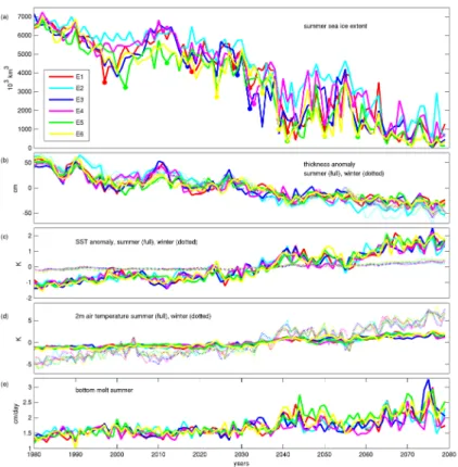
Spatial averages of seasonal means (JFM for winter and JAS for summer) for key variables have been calculated north of 70◦_{N over the sea ice covered area with at least} 15 % of ice coverage (Fig. 1). In all ensemble runs overall trends are clearly visible.

5

Over the 100-yr period 1980–2079, summer sea ice extent is decreasing (Fig. 1a), as is thickness (Fig. 1b) during summer and winter.

The increase of 2 m air temperature (T2M, Fig. 1d) is strongest during winter (8– 10 K). Winter sea surface temperature (SST, Fig. 1c) change is much more limited (about 0.5 K) due to the isolating ice cover and almost constant freezing point

tem-10

peratures directly underneath the ice. Summer T2M and SST are increasing both with roughly 2–3 K (note different ordinate scaling in Fig. 1) due to enlarged areas of leads and open water.

The strongest signal in melting and freezing rates is seen in the increasing summer melting at the ice bottom (Fig. 1e), which must be connected to water warming

under-15

neath the ice. A weaker increase is seen in the spring surface melting (no figure), while summer surface melting is decreasing. This is consistent with summer ice margins closer to the pole on average.

From the sea ice extent curve (Fig. 1a), it becomes clear that rapid loss events are followed by at least partial recoveries. This behavior is typical even for the observed

20

summer extent time series (e.g. Stroeve et al., 2008). It opens for the possibility of neg-ative feedbacks in response to the event. Alternneg-atively, it might indicate that conditions suitable for generating a loss event exist only for a limited number of years before less favorable conditions reoccur independently of the ice loss.

Variability on top of the trends show some intra-ensemble coherence on decadal

25

(9)

OSD

9, 2327–2373, 2012

Title Page

Tables Figures

◭ ◮

Back Close

Full Screen / Esc

Discussion

P

a

per

|

Dis

cussion

P

a

per

|

Discussion

P

a

per

|

Discussio

n

P

a

per

|

ensemble members show largely individual behavior with respect to occurrence of a rapid loss events, although clustering of 2–3 ensemble members occurs. After 2025, events are mostly clustered within at least 4 ensemble members in periods of 3–5 yr. This coherence suggests some degree of controlling by large scale conditions given by identical atmospheric conditions prescribed at the lateral boundaries of the regional

5

model domain. Still, even after 2025, a minority of cases does not participate in the clustering of events. Thus conditions and processes specific to the individual ensemble runs are essential and can overrule a dominating large scale influence emanating from identical lateral boundary conditions.

As an example of clustering, we take a closer look at the events during the period

10

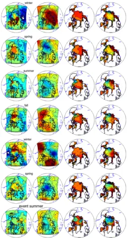
2030–2035 to learn about preferred conditions for clustering. During that period, 5 out of 6 members show an event, and the sixth member is close to an event. We com-pare the SLP of the event with a reference period of 10 yr before the event (Fig. 2). We consider the average winter before an event and the average event summer it-self. Both show a distinct high surface pressure anomaly over Alaska and northern

15

Canada. During winter, the high anomaly is complemented by a pronounced negative anomaly covering most of the Arctic ocean and centered over the Laptev sea reaching into northern Europe and Siberia. This indicates a broad inflow of air from the Pacific ocean into large parts of the central Arctic ocean and towards the Canada and Green-land coast, connected to sea ice drift from the Chukchi and eastern Siberian Seas

20

towards Canada and Greenland. During summer, the SLP anomaly is dominated by high pressure over the Beaufort Sea including the North American coast, and another high pressure anomaly over the wider Greenland area, which also gives rise to atmo-spheric inflow from the Pacific across the Arctic ocean. The summer sea ice thickness anomaly (Fig. 2c) shows strongest thinning in the Chukchi Sea, eastern Siberian Sea

25

(10)

OSD

9, 2327–2373, 2012

Title Page

Tables Figures

◭ ◮

Back Close

Full Screen / Esc

Discussion

P

a

per

|

Dis

cussion

P

a

per

|

Discussion

P

a

per

|

Discussio

n

P

a

per

|

ice reduction during the clustering phase is very much concentrated on the Siberian coastal Seas, while the 30-yr average shows reduction in almost all of the Arctic ocean. We conclude that atmospheric conditions supporting ice loss in the Siberian coastal Seas, provide a strong constraint to generate a RILE. Most of our 30 events show some ice left at the east-Siberian coast. This is a feature of many Arctic or global

cli-5

mate models (e.g. Gerdes and K ¨oberle, 2007; Blanchard et al., 2011). If this can be counteracted by specific large scale atmospheric conditions, we have a strong poten-tial for common RILEs within the ensemble, largely independent of local conditions or possible feedbacks.

Taking into account that thick ice off Siberia might be an unrealistic feature, given

10

existing high pressure biases (Cassano et al., 2011) and the e_ffects of not considering multiple ice classes (Vancoppenolle, 2008), the described dominance of large scale atmospheric conditions, as expressed by clustering in the model experiments, might be less important in reality.

4.2 The average rapid sea ice loss event

15

Sea ice rapid change events differ in the importance of specific mechanisms and the location of ice reduction. Analyzing an average event gives insights into dominating features valid for most events. More detailed understanding of processes needs to be derived from specific analysis such as composites (Sect. 4.4) and specific case studies (Sect. 4.5).

20

Here we present average seasonal anomaly fields over all 30 events including the year of the event. If an event consists of more than one step (i.e. several consecutive drops of summer extent in a row), all steps are taken into account and averaged into one average seasonal cycle of the event year. Each single anomaly field represents the di_fference between the respective season and the corresponding 10 yr seasonal mean

25

(11)

OSD

9, 2327–2373, 2012

Title Page

Tables Figures

◭ ◮

Back Close

Full Screen / Esc

Discussion

P

a

per

|

Dis

cussion

P

a

per

|

Discussion

P

a

per

|

Discussio

n

P

a

per

|

event. Resulting fields are shown in Fig. 3a for the event and in Fig. 3b for the recovery. Melting rates for bottom and top of the ice are given in Fig. 3c.

The average winter (JFM, Fig. 3a, upper row) before the average summer event shows a distinct T2M rise over all the Arctic ocean and adjacent land areas, with a maximum warming of up to 2 K over the Chukchi Sea. That warming appears to be

5

consistent with a winter SLP anomaly associated with warm air transport from the Pa-cific area into the Arctic. This corresponds to a weakening of the typical wintertime zonal transport in the Arctic. Other winter anomalies are rather small: sea ice concen-tration (SIC) reduction is limited to the winter ice margin. Winter sea ice thickness is reduced by up to 35 cm away from the northern Greenland and Canada coastal area.

10

SST anomalies (no figure) reflect SIC changes. The SLP anomaly shows similarities with Fig. 2 which represents the conditions of e_fficient large scale forcing of a RILE in the coming summer. A small but decisive difference is the weaker depression cen-tered over the Kara Sea implying no direct ice drift from the East-Siberian shelf towards Canada and Greenland.

15

During spring (AMJ, Fig. 3a, second row) before the summer event, T2M over the ice is still about 1 K warmer compared to the 10 yr average before. That anomaly cannot be related to warm air advection as during winter, because SLP anomalies cannot support such an argument. Instead, the T2M warming must be influenced by a reduced sea ice thickness as a result of the warm winter atmosphere. Thickness is reduced almost all

20

over the ocean with values around−30 cm in the central Arctic and maximum values of −70 cm. SIC is distinctly negative at the ice margin of the Barents Sea and the Beaufort Sea coast, but only slightly negative away from the margins. Again, SST anomalies are roughly following the SIC.

During summer (JAS, AVD, Fig. 3a, third row), sea ice concentration (SIC, here

ex-25

(12)

OSD

9, 2327–2373, 2012

Title Page

Tables Figures

◭ ◮

Back Close

Full Screen / Esc

Discussion

P

a

per

|

Dis

cussion

P

a

per

|

Discussion

P

a

per

|

Discussio

n

P

a

per

|

ice cover during the 100-yr-long model runs is also contributing to the only modest av-erage reduction values at the margin, as RILEs are increasingly occurring in the more central areas. SST warming again is following the pattern of SIC. Atmospheric sur-face temperature (T2M) is only slightly increased during summer in ice margin areas (coastal Beaufort Sea and north of Spitsbergen) , which are about consistent with a

5

high number of ice free summers among the 30 events in those areas. Over the re-maining ice, T2M is close to the freezing point.

The SLP anomaly during the summer event is given by an elongated high pres-sure ridge over the European and Eurasian coast, connected to an anomalous inflow of warm air from the Nordic Seas into the Arctic ocean. This is completely different

10

compared to the externally controlled cases as illustrated in Fig. 2, indicating influence of internal processes. Consequences of that average SLP anomaly on other average anomaly fields such as thickness or shape of ice cover cannot be detected here. How-ever, a similar pattern is found in composites of specific events with least extreme SIC reductions and least extreme winter warming, both connected to rather moderate loss

15

events of summer sea ice extent (no figure), indicating a role of this SLP anomaly pattern for modest loss events rather than for the most extreme events.

Summer sea ice thickness (in Fig. 3a expressed by September conditions) is reduced by up to 45 cm. Areas of biggest average thinning are not completely identical with ar-eas of strongest ice concentration reductions, indicating non-linearities due to different

20

mechanisms involved in the individual events, and due to very thick ice at parts of the Siberian coast. Case studies (Sect. 4.5) and composite analysis (Sect. 4.4), which explore individual events or groups of events, both show a better coherence between reductions of thickness and concentration.

Bottom melting during spring and summer (Fig. 3c) is increased in large areas.

25

(13)

OSD

9, 2327–2373, 2012

Title Page

Tables Figures

◭ ◮

Back Close

Full Screen / Esc

Discussion

P

a

per

|

Dis

cussion

P

a

per

|

Discussion

P

a

per

|

Discussio

n

P

a

per

|

During fall (OND, Fig. 3a), T2M over sea ice is much warmer than the average 10 yr before (up to 3–4 K). Anomalous atmospheric circulation can only support a part of that warming of the central Arctic by advection from the Nordic Seas. Due to the clear limitation of the strongest warming pattern to the ocean, a much reduced SIC and a diminished ice thickness must be the major reason for the warm air anomaly. Reduced

5

ice concentration and thickness during the last three months of the year is consistent with the view of a later start of the freezing season with subsequently less dense and thinner ice cover. Similar e_ffects have been observed after low-ice summers after year 2000 (Overland and Wang, 2010)

The average winter (JFM, Fig. 3b) after a summer event still shows anomalously

10

warm T2M over all the Arctic ocean, but the signal is smaller and more localized than during the foregone fall. SIC is largely back to normal with slightly increased concen-tration in the Greenland Sea, indicating a recovery of sea ice extent above the 10 yr reference period. Ice thickness is still below normal away from the Nordic Sea ice mar-gins. This can potentially contribute to the still warmer T2M, but horizontal patterns

15

do not coincide well. Instead the winter T2M anomaly is reminiscent of the previous fall SIC anomaly pattern, indicating a signal storage in the ocean surface temperature. SLP shows a low pressure anomaly over large parts of the Arctic and Nordic Sea area. The pattern is reminiscent of the positive phase of the Arctic Oscillation. The specific shaping tends to decouple the Arctic from the Pacific sector circulation, but in other

20

sectors allow for advective warming from southern latitudes, thus contributing to the T2M anomalies.

The following spring (AMJ, Fig. 3b) shows only minor anomalies for T2m and SLP. Sea ice thickness anomalies show persistence with thinner ice at the Siberian coast and in the Arctic interior (the transpolar drift area) compared to the reference period.

25

(14)

OSD

9, 2327–2373, 2012

Title Page

Tables Figures

◭ ◮

Back Close

Full Screen / Esc

Discussion

P

a

per

|

Dis

cussion

P

a

per

|

Discussion

P

a

per

|

Discussio

n

P

a

per

|

During the following fall (OND, Fig. 3a) T2M over the Arctic ocean is still anomalously warm over the ice, likely due to ice concentrations or ice thickness which are still below normal in the Arctic interior. SLP anomalies do rather not support advective influences. Reviewing the average development of the ice field, we see only slightly reduced SIC during the average winter (JFM) of the event year. During the event summer, maximum

5

reduction is reached. This is maintained even during the fall directly after the sum-mer event. The following winter, spring and sumsum-mer show only moderately negative SIC anomalies away from the ice margin. The interior ice thickness anomaly remains strongly negative during the complete two-year-period. Despite the only moderately negative SIC anomalies during the year after the event, we still find a strongly positive

10

T2M anomaly during the second fall after the summer minimum event. Thus the T2M fall anomaly is reoccurring after a spring and a summer without relevant T2M anoma-lies, while the sea ice extent and concentration are clearly recovering. As the fall T2M anomaly is largely limited to the ice-covered ocean area, its survival must be due to a signal storage mechanisms related to sea ice or ocean. In the winter after the event

15

we see effects of a warmer ocean underneath the ice. For the year after the summer minimum, Blanchard et al. (2011) suggest a re-occurrence by means of memory in the ice thickness, which has an annual or even longer time scale. We see no other mech-anism that could be responsible for the re-occurence. Accordingly, we suggest that the fall T2m signal reemerges because of the still anomalous ice thickness.

20

4.3 The role of the Arctic Dipole (AD) anomaly

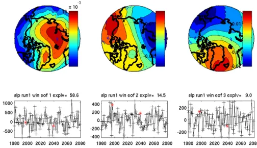
To find dominant modes of sea level pressure (SLP) variability over the Arctic, we cal-culate EOFs based on winter (JFM) means north of 70◦_{N for the complete analysis} period 1980–2079. A typical result is shown for scenario E1 (Fig. 4). The first EOF with a center over the Arctic ocean is dominating the variability with an explained variance

25

(15)

OSD

9, 2327–2373, 2012

Title Page

Tables Figures

◭ ◮

Back Close

Full Screen / Esc

Discussion

P

a

per

|

Dis

cussion

P

a

per

|

Discussion

P

a

per

|

Discussio

n

P

a

per

|

oscillation are located over North America and Siberia. The third mode with a smaller explained variability of 9 % is rotated by about 90◦ _{compared to the DA. (As an} alter-native definition based on larger SLP fields between 10◦_{N and 90}◦_{N, the DA would} result as the third principal component after AO/NAO and the Pacific North America anomaly PNA, Overland and Wang, 2010). The associated principal component time

5

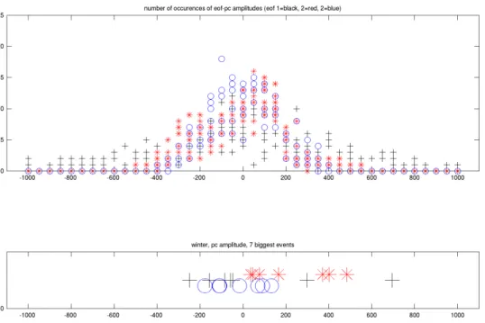
series show no significant long term trends, but annual-decadal variability. The distri-bution of the DA mode amplitudes for all 6 scenario experiments (Fig. 5, upper panel) shows a slightly skewed distribution with a maximum towards positive values. When selecting only the most extreme sea ice reduction events (Fig. 5, mid panel), we see exclusively positive amplitudes for the DA mode, while the leading AO mode and the

10

nameless third EOF mode give both negative and positive amplitudes. The opposite selection of the remaining reduction events give both negative and positive amplitudes for all three modes. Thus the most extreme rapid sea ice loss events are connected to positive DA anomalies during the winter before, which implies atmospheric warm inflow of Pacific origin into the Arctic. This finding is concordant with 2d composite results for

15

the 20 % most extreme cases (COMP, Fig. 6c), also indicating increased atmospheric inflow from the Pacific sector.

It becomes clear that the most extreme cases of sea ice extent drop require a positive DA phase. In reverse however, a positive DA phase does not guarantee a summer sea ice drop. Thus, a positive DA is a necessary, but not a su_fficient condition for an

20

extreme sea ice extent drop. This is again an expression of the role of meridionality for rapid change events.

Viewing the principal component time series in the example of Fig. 4e, the DA am-plitude is subject to interannual as well as to clearly visible interdecadal variability. Low phases are preventing strong extreme events.

25

4.4 Composites

(16)

OSD

9, 2327–2373, 2012

Title Page

Tables Figures

◭ ◮

Back Close

Full Screen / Esc

Discussion

P

a

per

|

Dis

cussion

P

a

per

|

Discussion

P

a

per

|

Discussio

n

P

a

per

|

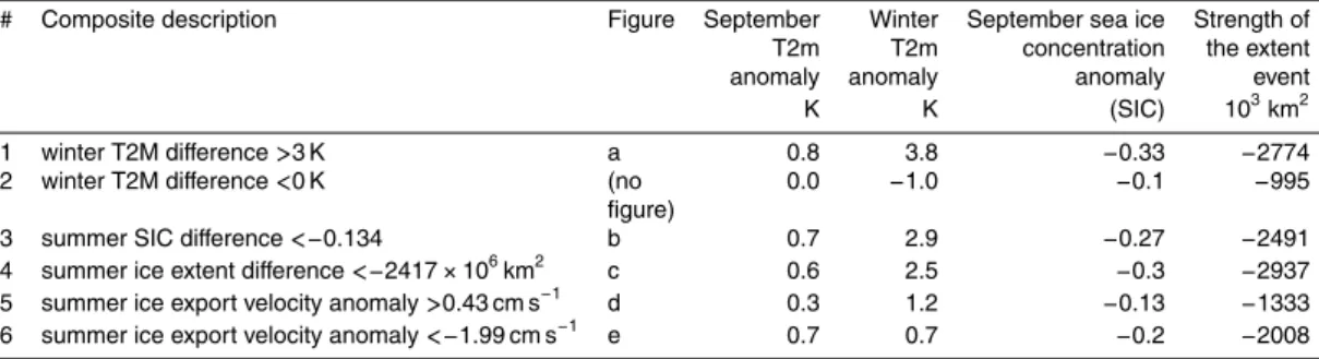
sea ice loss events. Selection criteria are chosen to cover the 20 % (6 out of 30 events) respective most extreme events. We define composites based on either summer (of the event) or winter (the winter before the event) conditions, and show resulting patterns for both winter and summer. Table 2 summarizes the different composites.

The composites #1 and #2 are defined by a warm resp. cold winter (JFM) 2-m-air

5

temperatures in comparison to the 10-yr reference period. Composite #1 covers air temperature anomalies greater than 3.85 K, corresponding to the six warmest cases. Fig. 6a shows the warming pattern which is connected to strongest anomalies of sum-mer sea ice concentration and sumsum-mer extent (−2744×103km2, see Table 1 for sea ice extent). This is even true for summer thickness (no figure). The winter SLP pattern

10

supports advection of warm air into the Arctic from both the Atlantic sector, from east-ern Europe and from the American west coast. In reverse, cold winters (composite #2, no figure) give moderate summer sea ice concentration reductions, connected with an isolating low pressure anomaly over the central Arctic. The reason why these cases still show a moderate rapid change event during summer, are to be found during summer

15

itself (“summer-driven cases”) when the SLP patterns like the one in Fig. 3a (“summer SLP”) supports advection of warm air from the Atlantic. Those summer SLP condi-tions are in general agreement with the 30-case-average description in section TWOD. Ice extent event values can be less than the original selection criterion of the event definition (1200×103km2) because the numbers here refer to average year-to-year

20

changes, while the event definition covers the cumulative e_ffect of up to 3 yr.

Small negative concentration anomalies at the ice margins in Fig. 6 might be counter-intuitive but can be explained by small concentrations even during the reference period directly before the event (which might be anywhere on the scenario time axis), and by spatially-different ice-free areas among the members of the composite.

25

(17)

OSD

9, 2327–2373, 2012

Title Page

Tables Figures

◭ ◮

Back Close

Full Screen / Esc

Discussion

P

a

per

|

Dis

cussion

P

a

per

|

Discussion

P

a

per

|

Discussio

n

P

a

per

|

composites can show stronger reductions. This composite is connected to a strong ex-tent reduction (Table 2), slightly smaller (∼400×103km2) than the most extreme com-posite. For this composite we find a winter SLP anomaly pattern quite similar to the “T2M>3.85 K” composite, indicating that winter atmospheric warming by atmospheric circulation indeed plays a major role for the most extreme summer sea ice

concentra-5

tions.

Composite #4 collects the most extreme drops of summer sea ice extent. Those drops (“d extent<₋2417_×103km2”, Fig. 6c) occur in connection with an air inflow anomaly from the Nordic Seas during summer and a surface air temperature anomaly over the ice during the winter before the event. The summer atmospheric circulation

10

anomaly is caused by a low pressure anomaly over Greenland and high anomalies over the Bering Sea and Kara Sea. It is the Kara Sea summer SLP anomaly pattern that dominates the all-event average during summer (Fig. 3a).

The winter SLP anomaly shows a tripod-like pattern with a low anomaly over the eastern Arctic and three high pressure anomalies over southern Siberia, the Nordic

15

Seas and Alaska. The pattern consisting of the Alaska high and the central low anomaly bears some resemblance of the Arctic Dipole Anomaly (DA) pattern (Wu et al., 2006) in its positive phase. Both positive DA and the tripole seen here are suitable to foster atmospheric inflow from the Pacific area into the Arctic. EOF analysis in section XX shows that indeed a strong positive state of DA oscillation is a necessary constituent

20

for an extreme RILE. It is the tripod-like winter SLP anomaly pattern which dominates the all-event-winter-average (Fig. 3a). In addition to the pure DA pattern, it brings warm air from the Pacific to the Arctic. An associated sea ice thinning (no figure) is centered in the Chukchi Sea and shows a horizontal pattern similar to the atmospheric warming anomaly.

25

(18)

OSD

9, 2327–2373, 2012

Title Page

Tables Figures

◭ ◮

Back Close

Full Screen / Esc

Discussion

P

a

per

|

Dis

cussion

P

a

per

|

Discussion

P

a

per

|

Discussio

n

P

a

per

|

summer, the “strong export” case is connected to a large scale SLP anomaly pattern with a low over the Norwegian and Barents Sea and a high over the western Arctic, indicating an atmospheric forcing of sea ice movement towards Fram Straits. In the opposite case (“weak export”, #6), events are connected to negative export anomaly, which is connected to a large scale SLP pattern of opposite polarity suitable to hamper

5

ice export.

Interestingly, the weak export composite #6 gives a stronger RILE than the export composite. This is due to anomalous advection of warm air into the Arctic during sum-mer, due to the pressure anomaly pattern. The warming effect is out-competing the effect of ice transport. The event amplitudes (2008×103km2for the weak export and

10

1333×103km2 for the strong export) both show moderately strong events. This indi-cates that the strength of sea ice export itself is not an important factor for generating rapid sea ice reductions in our model.

An additional composite pair (no figure) distinguishes one-step cases from two-step cases (see definition of events). Interestingly, the one-step composite gives figures

15

very similar to the weak export case (composite #6), confirming that strong single-step events require the summer inflow from the Atlantic sector. Two-step events are more dependet on the winter atmospheric circulation with SLP anomalies very similar to the strongest events in composites #1 and #4 .

Table 2 summarizes the composites. The relation between September SIC and

20

strength of the event is quite linear. As to be expected, the event strength increases both with winter and summer T2m. Note that the combination of warmest T2M anoma-lies for winter and September (composite #1) leads to a strong event, but is outrivaled by a combination of more moderate (but still strong) T2m anomalies (composite #4), pointing to influences of more detailed flow patterns and other effects.

25

4.5 Individual cases

(19)

OSD

9, 2327–2373, 2012

Title Page

Tables Figures

◭ ◮

Back Close

Full Screen / Esc

Discussion

P

a

per

|

Dis

cussion

P

a

per

|

Discussion

P

a

per

|

Discussio

n

P

a

per

|

one-step events as well as events in several steps, i.e. involving a series of consecutive ice reductions from summer to summer. Most cases involve more than one step.

For further examination, here we choose case 1 (with reduced ice in the Pacific and Atlantic sectors), case 16 (with reduced sea ice offthe Eurasian and Alaska coast), and case 26 (with reduced sea ice cover o_ffnorthern Canada during summer). Anomalies

5

in this section are referring to the di_fference between a specific season and the corre-sponding 10-yr average season directly before the event. If the case is a multiple-step event, the 10 yr reference period ends at the beginning of the first step.

Case 1 with a sea ice record minimum during summer 1998 is a one-step event in the ice extent. A sequence with seasonal means starting two winters before the summer

10

event are shown in Fig. 7.

The two preceding winters before the summer event both show anomalously warm atmospheric conditions over parts of the Arctic ocean. In both winters, the warm sur-face temperatures can be associated with atmospheric transport anomalies as inferred from SLP anomaly patterns. This is even true for the two falls before those winters. This

15

leads to generally thinner ice compared to the 10 yr average reference period. The sea ice thickness anomaly shows first signatures of the 1998 event already during the sum-mer 1997. An elongated low pressure anomaly centered over the pole is connected to ice drift away from the Chukchi Sea towards the Canada Basin. The resulting thick-ness anomaly pattern with thinner ice in the Chukchi and Beaufort Seas remains until

20

the event summer. T2m anomalies over the Chukchi Sea during fall 1997 and winter 1997/1998 reflect the reduced ice thickness, but are even supported by inflow of warm air from the Pacific and Siberia. This corresponds to a high amplitude of the winter AD anomaly pattern (amplitude 371). Thus, an important precondition in the winter before the summer event is fulfilled.

25

(20)

OSD

9, 2327–2373, 2012

Title Page

Tables Figures

◭ ◮

Back Close

Full Screen / Esc

Discussion

P

a

per

|

Dis

cussion

P

a

per

|

Discussion

P

a

per

|

Discussio

n

P

a

per

|

shallow low close to the warm anomaly (Walter et al., 2001). Alexander et al. (2004) find a local and direct baroclinic response to sea ice retraction connected to near-surface warming and below-normal sea level pressure.

During the event summer, a low pressure anomaly is concentrated in the Canada Basin and northern Greenland area (similar to the average event summer, Fig. 3a),

5

connected with atmospheric inflow from the Nordic Seas. The latter reduces sea ice concentration north of Laptev Sea. Both spring and summer 1998 show increased bottom melting (no figure). The fall and winter after the event show increased warming over large ocean and land areas. This warming reoccurs next fall due to still reduced ice thickness.

10

Summarizing, a generally thin ice already during 1997, assisted by an additional circulation-driven thinning during summer 1997 provided the preconditions for the 1998 event. The 1997 summer anomaly in the ice thickness survived the winter due to fa-vorite meridional atmospheric circulation and was enhanced during summer 1998 by anomalous meridional atmospheric flow from the Atlantic sector.

15

Case 16 is a three-step event with a first drop of ice extent in summer 2031 following several decades of smaller variability. A large step in 2032 is followed by an additional smaller final drop in 2033.

Similar to case 1, the falls and winters before the summer drop show positive T2M anomalies over the Chukchi and Siberian Seas, which can be explained by regionally

20

meridional atmospheric advection. Due to those repeated fall and winter conditions, initial negative ice thickness anomalies in the Chukchi and Siberian Seas survive and further develop all the way to the summer 2033. Two winters before the event (Fig. 8) show positive DA amplitudes, whereby the winter 2031/2032 shows the strongest DA value. Again and similar to case 1, an important precondition of strong meridionality

25

(21)

OSD

9, 2327–2373, 2012

Title Page

Tables Figures

◭ ◮

Back Close

Full Screen / Esc

Discussion

P

a

per

|

Dis

cussion

P

a

per

|

Discussion

P

a

per

|

Discussio

n

P

a

per

|

In line with the other cases, springs during this event are often characterized by low SLP anomalies in the central Arctic, connected to anomalously thin ice.

During the summers (2032 and 2033), bottom melting is clearly compared to the 10 yr average before the events. In principle this could be either due to reduced ice concentration and associated local water heating from the surface, or due to deeper

5

ocean influences. To examine those possibilities, we explore the spring and summer 2032, which shows a distinct positive SST (no figure) and negative ice concentration anomaly (Fig. Case16) in the Chukchi and East Siberian Seas.

Winds drive away the ice from and Chukchi Sea. Open waters occur, connected to immediate SST warming. A zone of increased bottom melting extends about 3 grid

10

boxes (about 150 km) under the ice and leads to additional ice concentration reduction until the wind driving stops. In that area of mixed ice and open water within individual grid boxes, the fraction of open water and bottom melting increases simultaneously. After an initial reduction of ice concentration, heat is absorbed by the upper ocean layer and immediately used for bottom melting, such that SST is not increasing for some

15

time. In the given example we see a time delay of about 10 days between ice fraction opening and SST response A mechanism similar in principle has been observed during the 2007 event by Perovich et al. (2008).

We also tested the idea of possible upward transport of ocean heat by vertical mixing in response to reduced ice concentration. No sign of such a process was found in this

20

model. We find locally increased vertical mixing at grid points with strongly reduced ice concentration, reaching down to several tens of meters, but the heat source is the surface, not the ocean.

Case 26 is a one-step event with a record sea ice extent minimum in 2025 after several decades of smaller variability on top of a downward trend. The actual event is

25

(22)

OSD

9, 2327–2373, 2012

Title Page

Tables Figures

◭ ◮

Back Close

Full Screen / Esc

Discussion

P

a

per

|

Dis

cussion

P

a

per

|

Discussion

P

a

per

|

Discussio

n

P

a

per

|

if the atmospheric and oceanic conditions allow. The initial sea ice thickness anomaly persists until the record ice extent event and is joining up on the way (during fall and winter before the summer event) with an additional ice thickness anomaly o_ffCanada, even that one generated by anomalous meridional winds from the south. The winter before the summer event shows a moderately positive AD amplitude which potentially

5

helps keeping the initial anomaly with winds from the Pacific almost parallel to the Canada coast. A few months later, during spring before the event summer, both initial sea ice anomalies grow. During summer, this leads to large areas of open water and low ice concentrations o_ffthe Canadian and northern Greenland coast reaching all the way to the Laptev sea, with ice remaining between the eastern Siberian coast and the

10

pole.

Thus, an important period for this event is the spring 2025, just a few months before the record summer. Increased spring thinning offCanada is related to an atmospheric low pressure anomaly covering the Beaufort Sea, the Bering Sea and larger coastal parts of Alaska and Canada. That anomalous atmospheric circulation pushes the ice

15

away from the coast towards the pole area, without suppressing the initial Laptev ice anomaly. A surface warming occurs as a consequence of ice retreat. This in turn sup-ports the further existence of the atmospheric low pressure anomaly, thereby potentially constituting a positive feedback. The summer shows the typical positive SLP anomaly (as seen in in 30-case average in Fig. 3a) over the Eurasian coast in a strong

realiza-20

tion.

Already during spring 2025, both bottom melting and surface melting increase com-pared the 10-yr reference period, whereby bottom melting is increasing more than sur-face melting. During the event summer, bottom melting is still increased due to heat entering the ocean leads.

25

(23)

OSD

9, 2327–2373, 2012

Title Page

Tables Figures

◭ ◮

Back Close

Full Screen / Esc

Discussion

P

a

per

|

Dis

cussion

P

a

per

|

Discussion

P

a

per

|

Discussio

n

P

a

per

|

atmospheric forcing. Also during spring we see a self-supporting low pressure anomaly which stabilizes ice melting and o_ffshore ice transports. Large scale circulation sets the stage for shaping the conditions for a strong ice loss event, but a local feedback contributes to the amplitude and shape of the ice extent drop.

Reviewing our three cases (cases 1, 16, 26), we find rapid ice change events with low

5

ice concentrations in di_fferent parts of the Arctic ocean. Each event is preconditioned by an initial sea ice thinning generated by an atmospheric circulation anomaly, often connected with northward transport of heat. Depending on the atmospheric conditions of the forthcoming seasons, the anomaly survives and grows during a period of 1–3 yr, modified by wind conditions and partly regional feedbacks. Events can be dominated

10

both from preconditioning or from summer atmospheric forcing conditions. After the event summer, atmospheric conditions favor a less meridional circulation leading to a partial recovery of sea ice. This is also found e.g. in the composite #4 of the most extreme events which gives a stronger SLP-anomaly-isolation over the ocean during the winter of recovery (no figure).

15

Each event is connected to increased bottom melting during the summer. The in-creased bottom melting is explained by large lead areas where atmospheric heat can be absorbed by the uppermost ocean layer and thereby contribute to bottom melt-ing. We see no indication for a bottom melting initiated by large scale heat fluxes in the ocean. Furthermore, we see no sign for decisive impact of radiative fluxes on triggering

20

ice events. Long wave radiation anomalies are merely reflecting surface air tempera-ture changes. Short wave solar radiation does not play a major role for generating the sea ice events in our model simulations. In the example of case 16 we see that the long wave downward radiation (no figure) hitting the surface is strongly reflecting T2M anomalies, which often are strongly positive over thinning ice, but is also affected by

25

(24)

OSD

9, 2327–2373, 2012

Title Page

Tables Figures

◭ ◮

Back Close

Full Screen / Esc

Discussion

P

a

per

|

Dis

cussion

P

a

per

|

Discussion

P

a

per

|

Discussio

n

P

a

per

|

5 W m−2_{is seen during the spring in regions with strongly reduced ice during the} com-ing summer. No correspondcom-ing signal in cloud cover can be found, and surface meltcom-ing is rather reduced. Thus, radiative changes play a minor role in our cases. However it should be noted that this finding is based seasonal means.

In most cases (case 1 and 26), a warm air anomaly in spring is connected to a

5

low pressure anomaly. In at least one case (case 26) we see indication for localized positive feedback between thin ice, connected to high surface air temperatures and a low pressure anomaly, which supports advection of new warm air into the area of thin ice. This is a self-supporting mechanism that helps keeping or strengthening the initial thickness anomaly. Warm air anomalies during winter are generally not connected to

10

low pressure anomalies at the surface. Fall and winter are more constrained by the large scale circulation. In this study, we are limited to surface variables. However the situation might look di_fferent for higher atmospheric levels. Overland an Wang (2010) show in a reanalysis-based study that sea ice reduction and warmer surface during fall leads to direct baroclinic signals e.g. in the the 1000–500 hPa thickness field, while

15

barotropic signals are more variable and thus not necessarily visible for the sea level pressure (SLP) fields in monthly or seasonal means.

Positive DA anomalies, identified here as a necessary but not sufficient winter pre-conditions for very strong events, clearly helps in all three cases. All cases show posi-tive DA anomalies, whereby two stronger ones are involved. Case 16 illustrates, that a

20

moderately positive DA supports the development towards the event, but the creation of the initial thickness signal is not connected to the DA.

5 Summary and discussion

We use a mini-ensemble of 6 different numerical Arctic climate scenario experiments each of 100 yr length to investigate a total of 30 rapid sea ice loss events.

25

(25)

OSD

9, 2327–2373, 2012

Title Page

Tables Figures

◭ ◮

Back Close

Full Screen / Esc

Discussion

P

a

per

|

Dis

cussion

P

a

per

|

Discussion

P

a

per

|

Discussio

n

P

a

per

|

addition to the general trend of of summer sea ice extent, we see decadal variability in all runs. Di_fferent variability timing within the ensemble would point towards pure local Arctic self-contained mechanisms (D ¨oscher et al., 2009). However, we find similar interannual and interdecadal variability of summer sea ice among ensemble members. Thus, summer ice extent is partly governed by global-scale atmospheric circulation,

5

which is enforced by lateral atmospheric boundary conditions (at the outer boundary of the regional model domain) identical to all regional runs. In addition to common variability, we see clustering of RILEs during certain periods in the di_fferent scenario experiments. Large scale atmospheric circulation supportive in reducing thick ice o_ff the Siberian coast, provides a strong potential for a RILE, so that many ensemble

10

members actually generate events.

In our model, ice in the Siberian Sea tends to be artificially thick as a result of insuf-ficient treatment of ice classes (M ˚artensson et al., 2012) and likely due to a high pres-sure bias over the Eurasian part of the Arctic ocean. This problem is shared with several GCMs (e.g. Vancoppenolle, 2008; Blanchard et al., 2011). Thus, results of this paper

15

might help interpreting GCMs. Given that the artificially thick Siberian ice blocks rapid ice loss events under atmospheric circulation regimes which do not oppose that exag-gerated thickness, it might be speculated that a more realistic geographical ice thick-ness distribution could lead to even more frequent rapid ice loss events in our model. Those might be less clustered within the ensemble. Our event case 26, timed during

20

2025, features a strong ice reduction o_ff northern Greenland and northern Canada connected to ice drift away from those coasts. In such a situation, a generally thinner ice offeastern Siberia can potentially lead to an even stronger event coming close to zero sea ice during summer. Thus, almost ice free summers could be possible even before 2040. In reverse and generally spoken: specific geographical thickness

distribu-25

tions compensate for atmospheric forcing which potentially could generate a rapid loss event.

(26)

OSD

9, 2327–2373, 2012

Title Page

Tables Figures

◭ ◮

Back Close

Full Screen / Esc

Discussion

P

a

per

|

Dis

cussion

P

a

per

|

Discussion

P

a

per

|

Discussio

n

P

a

per

|

by spring and summer atmospheric forcing. Winter conditions are preconditioning the coming summer, but not necessarily leading to an ice reduction event.

On average, rapid reduction events are characterized by increased temperatures over the ice during the winter before a summer event. Warmer air temperatures are caused by atmospheric circulation anomalies and impede sea ice growth, thus

lead-5

ing to less-than-average thickness already during that winter, whereby the average is represented by the respective 10 yr average before the start of the event year. Average spring temperature warm anomalies are related to the reduced ice thickness. Average summer conditions feature a high pressure anomaly along the Eurasian coast, and a slight negative anomaly over Greenland and the northern Canada coast, balancing

10

an anomalous atmospheric inflow from the Nordic Seas into the Arctic. The average summer event shows even increased melting at the bottom of the ice. Those average conditions give a very general picture because individual cases vary in mechanism and geographical location.

Studies of specific cases show that a winter thickness anomaly can already be

preex-15

isting in the winter before the summer event. In those cases, the atmospheric conditions during the year before are responsible for the initial thinning.

Composites of specific atmosphere and sea ice conditions reveal that the most ex-treme drops in sea ice extent occur in the combined case of winter atmosphere warm-ing and a summer cyclonic anomaly between the pole and Greenland. That summer

20

low anomaly is accompanied by high-pressure anomaly over the Kara Sea connected to inflow of air from the Nordic Seas into the central Arctic, and by a high-pressure anomalies over Alaska which turns the anomaly flow towards the northern Canada coast. More moderate RILE cases only show the Kara Sea summer anomaly.

The winter warming in extreme cases is supported by atmospheric inflow from the

25

(27)

OSD

9, 2327–2373, 2012

Title Page

Tables Figures

◭ ◮

Back Close

Full Screen / Esc

Discussion

P

a

per

|

Dis

cussion

P

a

per

|

Discussion

P

a

per

|

Discussio

n

P

a

per

|

conclude that the most extreme sea ice drops are not possible without a positive DA phase during winter. Analysis of observed sea ice reduction events point in the same direction: Wang et al. (2009) find record lows of Arctic summer sea ice extent to be triggered by the DA pattern. Observations also show a shift from largely zonal AO SLP patterns over the Arctic towards more DA-like meridional circulation patterns after

5

the millenium shift (Zhang et al., 2008). Reanalysis data sets show interannual and multi-annual variability of oscillation patterns in the Arctic (Overland and Wang, 2005). Concluding, decadal variability of the DA such as found in our model is a near-realistic feature and thus our runs suggests the possibility of alternating intensity of ice loss events in the future.

10

The only observed reference for our simulated RILEs is the 2007 sea ice record minimum event (e.g. Stroeve et al., 2008). As outlined in the introduction, atmospheric circulation anomalies dominated the event which was preconditioned by anomalously young and likely thin ice. The observed summer SLP pattern of below-normal pressure over Siberia and Laptev Sea and above-normal pressure over the western Beaufort

15

Sea and northern Canada corresponds to the strongly meridional flow carrying heat from subpolar latitudes (Ogi et al., 2008). Those factors in modified shape are shown to play a vital role in the simulated events of our model, even if the polarity is di_fferent from the specific year 2007. Kauker et al. (2009) show that winter preconditioning played a vital role for the 2007 event. In our model, that preconditioning is realized through warm

20

winters by means of large scale circulation anomalies.

Besides the DA, another expression of high pressure over northern Canada and the Beaufort Sea is the positive phase of the PNA, a wave train anomaly covering the North Pacific and the North-American west coast. In observations, both patterns (DA and PNA) are not correlated (e.g. Overland et al., 2008). Thus oscillations of the PNA

25

can potentially support or damp the amplitude of the DA which represents an important RILE forcing.

(28)

OSD

9, 2327–2373, 2012

Title Page

Tables Figures

◭ ◮

Back Close

Full Screen / Esc

Discussion

P

a

per

|

Dis

cussion

P

a

per

|

Discussion

P

a

per

|

Discussio

n

P

a

per

|

above. I.e. winters are not much warmer than the respective 10 yr reference period and atmospheric circulation shows only moderate meridional components. Ice thickness anomalies as created during the event, do not predetermine a continued reduction of summer extent.

The fact that we do not see a complete sea ice removal down to almost zero before

5

2040 in our model, could in principle be explained either by time limitation of supporting random winter and summer forcing conditions, which coincidentally do no occur more than 1–3 yr in a row, or by negative feedback mechanisms. A summer with little sea ice is always followed by a warm fall, and sea ice thickness anomalies can persist for several seasons. This gives a strong potential for another low-ice season the coming

10

summer. That potential is used e.g. in our simulated multi-step events, but it ceases mostly within 1–3 yr. Events longer that 3 yr are rare. In other cases, atmospheric circu-lation conditions do not support a further ice reduction, and thus, regular Arctic cooling mechanisms such as longwave upward radiation in combination with a less meridional atmospheric flow becomes the dominant influence. Reasons for a more zonal

circula-15

tion after the events might be a response to the anomalously warm Arctic. A reduced meridional temperature gradient, connected to reduced cyclonic activity in subpolar re-gions is suitable to reconstitute the large scale dynamic isolation of the Arctic. From the existence of both multi-year events and single-year events in our experiments we can conclude that no systematically dominating seasonal negative feedback exists in

20

our model.

Recovery after ice reduction is also seen regularly in the observed record of summer sea ice extent since 1979 (Stroeve et al., 2008). The ability of the sea ice to recover has also been demonstrated by Tietsche et al. (2011). A GCM is perturbed by complete removals of sea ice during summer. The response is a recovery back to the

centen-25