www.the-cryosphere.net/10/2999/2016/ doi:10.5194/tc-10-2999-2016
© Author(s) 2016. CC Attribution 3.0 License.
Quantification of ice production in Laptev Sea polynyas and its
sensitivity to thin-ice parameterizations in a regional climate model
Oliver Gutjahr, Günther Heinemann, Andreas Preußer, Sascha Willmes, and Clemens Drüe Department of Environmental Meteorology, University of Trier, Behringstraße 21, 54296 Trier, Germany Correspondence to:Oliver Gutjahr ([email protected])
Received: 6 April 2016 – Published in The Cryosphere Discuss.: 25 May 2016
Revised: 19 October 2016 – Accepted: 9 November 2016 – Published: 9 December 2016
Abstract. The quantification of sea-ice production in the Laptev Sea polynyas is important for the Arctic sea-ice bud-get and the heat loss to the atmosphere. We estimated the ice production for the winter season 2007/2008 (November– April) based on simulations with the regional climate model COSMO-CLM at a horizontal resolution of 5 km and com-pared it to remote sensing estimates. A reference and five sensitivity simulations were performed with different as-sumptions on grid-scale and subgrid-scale ice thickness con-sidered within polynyas, using a tile approach for fractional sea ice. In addition, the impact of heat loss on the atmo-spheric boundary layer was investigated.
About 29.1 km3 of total winter ice production was esti-mated for the reference simulation, which varies by up to +124 % depending on the thin-ice assumptions. For the most realistic assumptions based on remote sensing of ice thick-ness the ice production increases by+39 %. The use of the tile approach enlarges the area and enhances the magnitude of the heat loss from polynyas up to+110 % if subgrid-scale open water is assumed and by +20 % for realistic assump-tions. This enhanced heat loss causes in turn higher ice pro-duction rates and stronger impact on the atmospheric bound-ary layer structure over the polynyas. The study shows that ice production is highly sensitive to the thin-ice parameter-izations for fractional sea-ice cover. In summary, realistic ice production estimates could be retrieved from our simula-tions. Neglecting subgrid-scale energy fluxes might consid-erably underestimate the ice production in coastal polynyas, such as in the Laptev Sea, with possible consequences on the Arctic sea-ice budget.
1 Introduction
The rate of sea-ice growth strongly depends on the energy fluxes at the ice or ocean surface. If the total atmospheric heat flux is negative, the ocean loses heat either directly to the atmosphere or via conduction through an existing sea-ice cover. In the former case frazil ice forms, which aggregates subsequently to a new thin-ice layer under calm conditions. In the latter case basal freezing occurs to balance this heat loss. Most of the heat loss from the ocean occurs over open water or thin-ice areas, such as leads and polynyas, within an otherwise compact sea-ice cover (Smith et al., 1990; Morales Maqueda et al., 2004). Although the fraction of such areas in polar oceans is relatively small during winter, they are of ma-jor importance for the heat budget of the atmospheric bound-ary layer (ABL) (Heinemann and Rose, 1990; Haid et al., 2015) and the ocean circulation, such as the Arctic circumpo-lar boundary current (e.g. Aksenov et al., 2011; Rudels et al., 1999).
Quasi-stationary latent-heat or flaw polynyas reoccur fre-quently along the Siberian coast and along the fast-ice edge (Dmitrenko et al., 2001; Krumpen et al., 2011; Bareiss and Görgen, 2005) due to offshore wind stress (Smith et al., 1990; Dmitrenko et al., 2001; Morales Maqueda et al., 2004; Krumpen et al., 2011; Willmes et al., 2011a; Dmitrenko et al., 2012). These polynyas are narrow, long bands of open wa-ter and/or thin ice, which separate landfast ice from seaward drifting ice on the Siberian continental shelves during win-ter (Dethleff et al., 1998), predominantly from October until June (Bareiss and Görgen, 2005). In general, the ice cover in the Laptev Sea can be divided into three regimes: fast ice, pack ice, and flaw polynyas in between (Eicken et al., 2005). Particularly in winter, sea water at the freezing point is di-rectly exposed to a cold atmosphere, resulting in intense ice formation (Dethleff et al., 1998). Due to this strong surface heat loss within coastal polynyas frazil ice forms, which is subsequently transported toward the downwind edge of the polynyas (Smith et al., 1990; Morales Maqueda et al., 2004; Krumpen et al., 2011; Willmes et al., 2010). This process cre-ates a spatial gradient of thin-ice thickness (TIT) increasing from open-water conditions at the windward polynya edge to thicker ice at the downwind side. Here, at the polynya edge, the advected frazil ice accumulates to a thin layer (Martin and Kauffmann, 1981; Krumpen et al., 2011), which thickens and consolidates before it drifts further offshore. During the ice formation, salt is excluded from the ice matrix and is drained as brine from the sea ice (Krumpen et al., 2011). This salt in-put induces haline convection and erodes the density stratifi-cation of the underlying water column (Ivanov and Golovin, 2007; Bauch et al., 2009) and, if penetrative, dense bottom water forms (Backhaus et al., 1997; Bauch et al., 1995). The long-term mean probability for convective mixing down to the seafloor is only about 20 % in the western and about 70 % in the eastern Laptev Sea (Dmitrenko et al., 2005; Krumpen et al., 2011), which is owed to the general preservation of the stratification throughout the winter caused by freshwa-ter input from the Lena River during summer (Bauch et al., 2009; Dmitrenko et al., 2005). The cold, dense bottom water contributes to the Arctic halocline (Bauch et al., 2009) and thermohaline structure in the Eurasian Basin (Johnson and Polyakov, 2001).
The horizontal resolution of regional climate models is generally too coarse to represent leads and small polynyas explicitly. Therefore, they have to be treated as inhomo-geneities of momentum and energy fluxes on a subgrid scale. Heinemann and Kerschgens (2005) investigated three ap-proaches to account for such subgrid-scale inhomogeneities within a model grid box: the (i) aggregation, (ii) mosaic, and (iii) tile approach (TA). In the aggregation approach the pa-rameters for the fluxes (such as roughness length or albedo) are weight-averaged over different surface types within a grid box and then the fluxes are calculated from these grid-scale means. In contrast, in the mosaic approach the fluxes are ex-plicitly calculated on a sub-scale grid and averaged
after-wards. In the standard version (v5.0_clm1) of the regional climate model COnsortium for Small-scale MOdel – Climate Limited area Mode (COSMO-CLM or CCLM; Rockel et al., 2008), which is the climate version of the numerical weather prediction model COSMO of the German Meteorological Service (Steppeler et al., 2003), a model grid box is assumed to be either completely covered with sea ice or completely ice free. However, if neglecting subgrid-scale energy fluxes or heat loss from open-water or thin-ice areas, the energy transfer is underestimated and subsequently also the sea-ice production (IP). This underestimation affects the sea-ice bud-get and associated processes connected to the ocean, such as salt release and deep water formation (Martin and Cavalieri, 1989; Bauch et al., 1995; Ivanov and Golovin, 2007). Al-though the ocean processes are not represented in CCLM, the quantification of IP can be seen as a proxy for dense wa-ter formation.
In other regional climate models, such as the Polar Weather Research and Forecasting (Polar-WRF) model, frac-tional sea ice is already a default option with the assumption of subgrid-scale open water and with fixed sea-ice concentra-tions (SIC) and ocean temperatures during a 48 h simulation (Bromwich et al., 2009). However, assumptions have to be made for the subgrid-scale thin-ice thickness, since particu-larly in winter leads and polynyas are rarely ice free (Willmes et al., 2010, 2011a; Adams et al., 2013).
In the following we quantify the sea-ice production in the Laptev Sea polynyas (Siberia) and investigate its sen-sitivity on the assumptions of thin-ice thickness associated with the tile approach. The sea-ice module of Schröder et al. (2011) was already successfully applied in the Laptev Sea by Ebner et al. (2011), who could show that polynyas sig-nificantly affect the ABL. More recently, Bauer et al. (2013) calculated sea-ice production rates for this region based on COSMO simulations with an assumed thin-ice thickness of 10 cm (B10) or open water (B00) within polynyas. Their model results showed that the presence of grid-scale thin ice affects the IP considerably.
The implementation of a TA for subgrid-scale energy fluxes constitutes, from a physical point of view, an im-provement to the representation of polynyas in regional cli-mate models. However, it is unclear how sensitive the energy fluxes, the resulting IP, and the ABL are to the choice of grid-scale and subgrid-grid-scale ice thickness. By varying the thin-ice thickness in a sensitivity experiment, we aim to quantify these uncertainties. As a benchmark for our study we use the IP estimations of Willmes et al. (2011a, b). We further com-prise model results of Bauer et al. (2013) and derived IP from Moderate Resolution Imaging Spectroradiometer (MODIS) data.
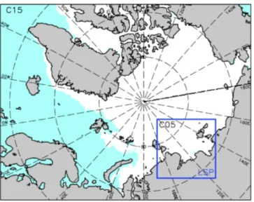
Figure 1.Model domains of COSMO-CLM at a horizontal resolu-tion of 15 km (C15, whole Arctic). The study domain of the Laptev Sea polynyas (LSP) with a resolution of 5 km (C05, blue box) is shown in detail in Fig. 2. The sea-ice extent (white shaded) is from 4 January 2008.
atmospheric boundary layer and on ice production rates are presented in Sects. 5 and 6 and discussed with respect to re-mote sensing estimates in Sect. 7. Finally, we conclude in Sect. 8.
2 CCLM configuration and model domains
The domain of CCLM (Fig. 1) covers the whole Arctic at a horizontal resolution of 15 km (C15). CCLM was run on 450×350 grid boxes and with 42 vertical layers, of which 16 are below 2 km height. Nested within, we performed sim-ulations for the Laptev Sea (Fig. 2 and Table 1) at 5 km resolution (C05) with 260×260 grid boxes and 60 verti-cal levels, of which 24 levels are below 2 km height. We subdivided this domain into four polynya regions, which have been already used in previous studies, e.g. by Willmes et al. (2011a): the north-eastern Taimyr polynya (NET), the Taimyr polynya (T), the Anabar–Lena polynya (AL), and the western New Siberian polynya (WNS). The total area of the masks is 26.19×10⁴km2.
The C15 model is forced by ERA-Interim data (Dee et al., 2011) with updates to the lateral boundaries every 6 h. The C05 models are then forced by the output of C15 with an update frequency of 1 h. The models were run in a fore-casting procedure for the winter period November 2007 to April 2008 (182 days in total). They were restarted every simulation day at 18:00 UTC and simulated the following 30 h. Thereby the initial sea-ice conditions (see Sect. 3.2) were prescribed to the sea-ice concentration and thickness of the following day. The first 6 h were cut off as spin-up. The
Figure 2.Model domain at 5 km resolution (C05) over the Laptev Sea (approximately 1500 km×1500 km) with the sea-ice concen-tration from AMSR-E showing open polynyas (≤70 %) on 4 Jan-uary 2008. Four polynya regions are superimposed as orange poly-gons: north-eastern Taimyr polynya (NET), the Taimyr polynya (T), the Anabar–Lena polynya (AL), and the western New Siberian polynya (WNS). A→B denotes the 214 km long cross section (ma-genta) used in Sect. 5. The locations of the four AWS stations are marked with green triangles.
simulation output (00:00–23:00 UTC) was stored at a tempo-ral resolution of 1 h.
Surface fluxes were calculated by a bulk transfer scheme with a stability dependence (Louis, 1979) (see Appendix B3). The vertical diffusion was parameterized by a level-2.5 clo-sure scheme (Mellor and Yamada, 1974) based on a prog-nostic equation for turbulent kinetic energy (TKE). Radiation processes were calculated hourly using the Ritter and Geleyn (1992) scheme extended for ice clouds. We applied a Runge– Kutta scheme of third order (Wicker and Skamarock, 2002). Additionally, a fast-wave solver for sound and gravity waves was used (Baldauf, 2013). All simulations were run without spectral nudging.
Table 1.Overview of the performed simulations with COSMO-CLM for the winter period 2007/2008. The grid-scale thin-ice thickness (TIT) within polynyas (ice concentration: 0<SIC≤70 %) is shown in centimetres and the assumed subgrid-scale TIT is shown in parentheses. The latter is only required if the tile approach (TA) is used.
Model run 1x Region TIT[cm] TA Information
C15 15 km Arctic 10 (–) no forced by ERA-Interim
C05-ref 5 km Laptev Sea 10 (–) no reference run
C05-10/0 5 km Laptev Sea 10 (0) yes subgrid-scale open water C05-10/1 5 km Laptev Sea 10 (1) yes
C05-10/10 5 km Laptev Sea 10 (10) yes C05-50/5 5 km Laptev Sea 50 (5) yes
C05-50/1 5 km Laptev Sea 50 (1) yes realistic assumptions
location. According to Heinemann and Kerschgens (2005) the TA provides similarly good results as the mosaic ap-proach, but with distinctly less computation time. Thus, we decided to implement this variant. First steps in the direc-tion of a tile approach in CCLM were made by Van Pham et al. (2014). However, their adjustments were limited to area-weighted albedo values and to surface roughness values within a grid box that is covered with fractional sea ice. Al-though points (ii)–(iii) represent new modifications to CCLM as well, we accept them as the default option for our simula-tions.
The C15 simulation was performed without a TA in order to introduce effects from the TA only through the 5 km simu-lations. In case of C05, we performed a reference simulation in the Laptev Sea area without a TA (C05-ref) and five sensi-tivity simulations with the TA. The configuration of the ref-erence simulation is similar (as far as possible) to the config-uration of the previous studies of Bauer et al. (2013), where no TA was available. However, they used an older model ver-sion, which causes differences. C05-ref is thus comparable to the simulations of Bauer et al. (2013) and further the refer-ence without TA for our sensitivity simulations.
While the sea-ice thickness outside the polynyas was spec-ified as explained in Sect. 3.2, the ice thickness within the polynya areas has to be prescribed. For C15 and C05-ref the ice thickness in polynyas areas is generally 10 cm, but we as-sume 1 cm thin ice at polynya grid boxes in C05-ref, where the sea-ice concentration is 0 %. Such areas particularly pro-duce new ice and consist of a mixture of open water, grease and frazil ice, and thin solid ice. However, in winter open-water areas occur mostly at the windward side of polynyas, which is only a small fraction of the entire polynya area.
For three of the five sensitivity simulations we assumed also a grid-scale ice thickness of 10 cm for polynyas and assumed either subgrid-scale open water (C05-10/0) or a subgrid-scale TIT of 1 cm 10/1) and 10 cm (C05-10/10). The fourth and fifth sensitivity simulations were configured with a grid-scale ice thickness of 50 cm and a subgrid-scale TIT of 5 cm (C05-50/5) or 1 cm (C05-50/1). See Table 1 for an overview of the simulations. The assump-tion of 10 cm TIT originates from the fact that the mean
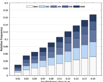
Figure 3.Thin-ice thickness distribution (≤20 cm) in the Laptev Sea derived from MODIS data for the winter periods (November– March) 2002/2003–2014/2015. The bars indicate the relative distri-bution of each thickness class from the total number of TIT≤0.2 m appearances between the winter seasons 2002/2003 and 2014/2015. Contributions of each month with respect to the whole winter sea-son for each thickness class are indicated by the blueish colours (see the legend). The mean thickness (±1 standard deviation) in this period is 13.5±0.5 cm (8.7 cm for≤10 cm). In the winter pe-riod 2007/2008, the mean is 14.0±2 cm (7.7 cm for≤10 cm).
TIT below 20 cm, derived from MODIS data, is of the order of≈10 cm. Willmes et al. (2011a) derived a mean thin-ice thickness of 11.6 cm for November to April (1979–2008), while from the MODIS TIT histogram in Fig. 3 a mean thin-ice thickness of 13.5 cm for November to March in the period 2002/2003–2014/2015 and of 14 cm for the winter 2007/2008 results, respectively. In a previous study by Bauer et al. (2013) 10 cm was thus assumed to be a realistic value for the thin-ice thickness within Laptev Sea polynyas. For better comparisons we assumed 10 cm as well in our refer-ence simulation (and in two sensitivity runs).
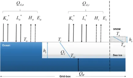
Figure 4. Scheme of the modified two-layer thermodynamic sea-ice module of Schröder et al. (2011), extended with a tile approach for fractional sea ice. Sea ice is distinguished as bare ice or as snow-covered ice (withhs=0.1 m snow depth if sea-ice thicknesshi>0.2 m). The subgrid-scale open ocean fraction is either ice free 10/0) or assumed to be covered with 1 cm 10/1, C05-50/1), 5 cm (C05-50/5), or 10 cm thin ice (C05-10/10). In the reference simulation (C05-ref), grid boxes with 0 % sea-ice concentration are covered with 1 cm grid-scale thin ice. If the indexkdenotes either sea ice (i) or ocean (o), thenQA,kis the total atmospheric heat flux,Kk∗is the net shortwave,
andL∗kthe net longwave radiation.Hk andEk are the sensible and latent heat fluxes.Tkis the surface temperature,hithe ice thickness, Toithe ice–ocean interface temperature, andTsithe snow–ice interface temperature.QIdenotes the conductive heat flux through the ice and QWthe turbulent heat flux from the oceanic mixed layer into the ice.
C05-50/5 and C05-50/1 runs are motivated by the fact that the sea-ice cover in the marginal ice zone consists of thicker ice floes (>20 cm) (detected by microwave satellite sensors) and thin ice (here the assumed 5 or 1 cm), which is not de-tected by microwave sensors. Thus we denote C05-50/1 as the simulation with “realistic” assumptions based on MODIS TIT.
Although this is a crude simplification to the real sea-ice thickness, it is suited for our purpose to investigate the im-pact on the magnitude of ice production and on the modi-fication of the ABL. We intended to consider sea ice in a computational cheap approach that still incorporates realis-tic thermodynamical processes. For a more sophisrealis-ticated ap-proach, a full dynamic–thermodynamic sea-ice model needs to be coupled to CCLM.
3 The two-layer thermodynamic sea-ice module 3.1 Basic module
In this section the sea-ice module (Fig. 4) is briefly described. The module considers a snow and sea-ice layer and was de-scribed and originally implemented in the COSMO model by Schröder et al. (2011). It is based on the module of Mironov et al. (2012). For this study it is reimplemented within the version 5.0_clm1 of CCLM extended with the Køltzow sea-ice albedo scheme (see Appendix A). More important for this study is the implementation of a tile approach for the sur-face energy balance over fractional sea ice (see Appendix B). The module and hence sea-ice growth calculation is only
ap-plied to grid boxes with an initial sea-ice cover. Formation of grease ice in open water is not parameterized in CCLM, which is a difficult task even for stand-alone sea-ice ocean models. Nevertheless, a more sophisticated parameterization has been recently developed by Smedsrud and Martin (2015). For this reason we calculated sea-ice production in a post-processing step (see Sect. 3.4).
The module assumes a constant ocean/ice interface tem-perature ofToi= −1.7◦C; i.e.Toiis not dependent on
salin-ity. A temperature of−1.7◦C assumes approximately a
salin-ity of 31.1 psu. The module ignores turbulent heat fluxes from the ocean at the lower boundary. Heat conductivity pa-rameters are 2.3 W m−1K−1for sea ice and 0.76 W m−1K−1
for snow. The module assumes a snow cover ofhs=0.1 m if the ice thickness exceeds a thresholdhi> hcwithhc=0.2 m. 3.2 Sea-ice concentration and thickness for initial
conditions
SIT is taken from the PIOMAS data set (Zhang and Rothrock, 2003). The PIOMAS data are available on a daily basis with a mean grid spacing of about 25 km (Hines et al., 2015). These daily fields were masked with the daily SIC fields to obtain consistent sea-ice extents. Thereby sea ice outside the AMSR-E mask was removed and grid boxes which were ice free in the daily PIOMAS fields but covered with ice in the mask were assigned with an interpolated SIT from a nearest neighbour method.
Schweiger et al. (2011) state that PIOMAS seems to over-estimate thin-ice thickness and underover-estimates thicker ice. Nevertheless, the overestimation should not be problematic in our application, since we have to set TIT for daily fields according to AMSR-E data. Underestimations of thicker ice is of minor concern to our study due to the focus on areas with thin ice. Using this setup, the sea-ice thickness fields are much more realistic than in previous studies, where a con-stant thickness of 1 m was assumed outside polynyas (Ebner et al., 2011; Schröder et al., 2011; Bauer et al., 2013). 3.3 Polynya area
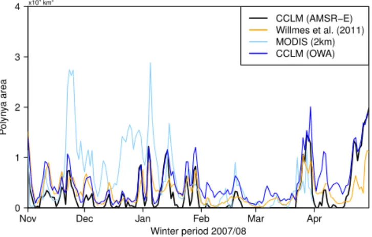
In Fig. 5 daily polynya areas for the winter period 2007/2008 are shown. According to the AMSR-E data set, which has been used to prescribe the SIC in CCLM and in the COSMO simulations of Bauer et al. (2013), large polynya events (>104km2) occurred at the end of November, in Jan-uary, and in March/April. The polynya areas of Willmes et al. (2011a) are approximately of the same order as those used for CCLM, whereas the retrieved polynya areas from MODIS2km are considerably larger. This discrepancy is caused by different threshold definitions for polynyas and by different horizontal resolutions. For the MODIS2km data, polynyas were defined as areas with thin ice,≤20 cm, as in Preußer et al. (2015b). Given that and the higher horizon-tal resolution it is likely that also leads within the polynya masks, not resolved by the microwave satellite data, are con-tributing to the total thin-ice area and hence larger areas re-sult. If areas of open water outside polynyas are considered as well, then the potential area for ice production increases in CCLM up to the area derived from MODIS2km data, ex-cept in the period of late November to the middle of Jan-uary, which remains lower. Another difference between the polynya area derived from CCLM and in particular the area from Willmes et al. (2011a) is that the latter nearly never drops to zero during this winter.
3.4 Estimation of sea-ice production
In accordance to previous model or satellite-based studies, IP was calculated in a post-processing step using the energy balance (Bauer et al., 2013; Ebner et al., 2011; Willmes et al., 2011a). This approach assumes that if the water within a polynya is at the freezing point, all energy loss to the atmo-sphere through the ocean surface is compensated by freezing.
0 1 2 3 4
Winter period 2007/08
P
olyn
y
a area
x104km2
Nov Dec Jan Feb Mar Apr
CCLM (AMSR−E) Willmes et al. (2011) MODIS (2km) CCLM (OWA)
Figure 5.Total daily polynya area interpolated from AMSR-E (us-ing a 70 % threshold) onto the CCLM 5 km grid in the Laptev Sea for the winter period 2007/2008 aggregated for the four polynya masks. In addition, the polynya area plus open-water area (OWA=1−SIC) for the polynya masks is shown. Based on remote sensing the polynya areas estimated from Willmes et al. (2011a) and MODIS2km data are shown. The total area of the polynya masks is 26.19×10⁴km2.
Hence sea-ice growth only occurs if the total atmospheric energy flux over ice (index k=i) or ocean (index k=o) QA,k=Kk∗+L∗k+Hk+Ek is negative, i.e. the ocean loses
heat: ∂hi
∂t = − QA,k
ρi·Lf, (1)
withhithe sea-ice thickness,ρi=910 kg m−3the density of
sea ice, and Lf=0.334×10⁶J kg−1 the latent heat of
fu-sion. We restricted this estimation to the four polynya areas in the Laptev Sea (see Fig. 2), which are identical to those of Willmes et al. (2011a). Hence, direct comparisons of our results with estimations from remote sensing were possible.
We further calculated the IP using the MOD/MYD29 sea-ice surface temperature product (Hall et al., 2004; Riggs et al., 2006) derived from MODIS Terra and Aqua data. In combination with ERA-Interim data (2 m temperature, 2 m dew point temperature, 10 m horizontal wind components, and pressure at mean sea level), an energy balance model (e.g. Yu and Lindsay, 2003; Adams et al., 2013; Preußer et al., 2015a, b) was applied to derive thin-ice thicknesses up to 0.2 m at a horizontal resolution of about 2 km. We refer to this estimation as MODIS2km. The turbulent fluxes of sen-sible and latent heat were calculated by an iterative bulk ap-proach (Launiainen and Vihma, 1990) based on the Monin– Obukhov similarity theory. Thereby, the turbulent exchange coefficientCHis a function of stability and of the roughness
2006). Therefore the number of useful swaths per day is vari-able. For instance, in the Laptev Sea there are about 10 to 14 swaths per day (2002/2003 to 2014/2015 – November– March).
Cloud-induced gaps in our daily sea-ice surface tempera-ture and thin-ice thickness composites were filled by a spatial feature reconstruction procedure (Paul et al., 2015; Preußer et al., 2015a). This method interpolates information of previ-ous and subsequent days to fill gaps caused by cloud cover. Based on these corrected composites and using the method described in Preußer et al. (2015b), ice production rates were calculated for each pixel with an ice thickness≤0.2 m, i.e. for polynya areas.
In a sensitivity analysis of this method (without the spa-tial feature reconstruction), Adams et al. (2013) stated an un-certainty for the ice-thickness retrieval of ±1.0, ±2.1, and ±5.3 cm for thin-ice classes of 0–5, 5–10, and 10–20 cm, respectively. Therefore, we constrained our analysis to ice thicknesses≤0.2 m, as this range is regarded as sufficient to get reliable results for ice production (Yu and Rothrock, 1996; Adams et al., 2013).
Furthermore, we compared our results to the estimations of Willmes et al. (2011a). In their study they used a con-stant transfer coefficient for heat CH=3×10⁻³ to
cal-culate H and E from AMSR-E data and using MODIS thin-ice distributions and National Centers for Environ-mental Prediction/National Center for Atmospheric Re-search (NCEP/NCAR) reanalysis data (2.5◦×2.5◦) as
atmo-spheric forcing for an energy balance model. However, we omitted the most western polynya mask of their study and compared the IP only to the four remaining masks shown in Figs. 1 and 2.
We also compared our IP estimations to model-based esti-mations of Bauer et al. (2013). Bauer et al. (2013) conducted two COSMO simulations at 5 km horizontal resolution (with-out a tile approach) for the same winter 2007/2008 in the Laptev Sea. One simulation assumed a grid-scale thin-ice thickness of 10 cm within polynyas (B10) and one simula-tion assumed open water (B00). Both simulasimula-tions further as-sumed a sea-ice thickness of 1 m outside polynyas. Both sim-ulations were forced by a 15 km COSMO simulation, which was nested within the output of the global GME model.
4 Evaluation with in situ data
The model output of the reference and the five sensitivity simulations were first evaluated with in situ data. During the Transdrift XIII-2 expedition from 11 to 29 April 2008 four automatic weather stations (AWS, Table 2) were deployed on the fast ice of WNS (see Fig. 2) (Heinemann et al., 2010). The AWS measured wind speed and direction at 3 m height with an accuracy of 2 % in speed and 3◦ in direction, air
temperature and relative humidity at 2 m height with and ac-curacy of 0.5 K and 4 %, and pressure with an acac-curacy of
Table 2.Overview of the four automatic weather stations (AWS) with hourly measurements which were deployed during the Trans-drift XIII-2 expedition from 11 to 29 April 2008 (Heinemann et al., 2010). See the location of the AWS in Fig. 2.
Station Location Measured period (UTC)
AWS1 128.16◦E 11 Apr 2008 07:00–26 Apr 2008 12:00
73.80◦N
AWS2 129.32◦E 12 Apr 2008 04:00–29 Apr 2008 03:00 74.39◦N
AWS3 131.25◦E 14 Apr 2008 06:00–29 Apr 2008 01:00 74.67◦N
AWS4 128.61◦E 24 Apr 2008 06:00–28 Apr 2008 02:00 74.05◦N
1 hPa. Furthermore, net radiation was measured by a net ra-diometer with an accuracy of 5 W m−2.
Here, we compared hourly C05 data with the AWS data. In order to judge whether the simulations deviate signifi-cantly from the AWS data two-sidedt tests were performed (α=95 %). The statistical comparisons were only performed for data pairs without missing values and only for days when the SIC was>95 %. This limitation is necessary because the time series of CCLM represent spatial averages of a grid box, whereas the AWS time series are point data on a solid ice cover. If the SIC of CCLM is<100 % then the grid aver-age automatically differs from the station time series, which always represent conditions at 100 % SIC.
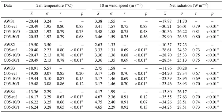
Table 3 shows the results for the reference simula-tion (C05-ref) and two sensitivity simulasimula-tions: C05-10/0 (subgrid-scale open water) and C05-50/1 (realistic assump-tions). In the remainder of the paper, we concentrate on the comparison of these three simulations. Since the comparison was made only over a solid sea-ice cover, the other simula-tions showed very similar results (not shown).
In general, the inter-model differences are minor for all variables. The comparison for the 2 m temperature shows that the C05 simulations are generally able to reproduce the observed temperatures during the measurement period. The temporal correlation is aboutr=0.8, except for the compar-ison with AWS4. The bias is about−1◦C for AWS2–3, less
for AWS1, and about−3◦C for AWS4. Except for the
lat-ter, C05 underestimates the variability of the 2 m tempera-ture. This might be caused by the assumptions made on snow properties in C05. Although thettests are significant for dif-ferences of about 1◦C, this difference is sufficient for our
analysis keeping in mind that grid-box averages were com-pared with point data.
In case of wind speed there is a good agreement (r≥0.7), although we compared 10 m wind speed of CCLM with mea-surements at 3 m height. The mean and standard variance are both in accordance with the AWS data, although significant for differences≥0.4 m s−1. Inversely, this agreement implies
Table 3.Statistical comparison of 2 m temperature, 10 m wind speed (3 m in case of the AWS), and net radiation (K∗+L∗) of the four AWS and the C05 simulations: C05-ref (reference), C05-10/0 (open water), and C05-50/1 (realistic). Hourly means are denoted byxand standard deviations are denoted byσ. The Pearson correlation coefficient (r) was calculated with the AWS and C05 time series. The critical correlation coefficient (α=5 %), which depend on the sample size of the AWS time series, is between 0.1 and 0.2. In addition, the resulting pvalues (p) of two-sidedttests (α=5 %) are shown. Significant differences are marked with∗. Data pairs with missing values in the AWS data or where the sea-ice concentration is<95 % were removed prior to the analyses.
Data 2 m temperature (◦C) 10 m wind speed (m s−1) Net radiation (W m−2)
x σ r p x σ r p x σ r p
AWS1 −20.44 3.24 – – 3.38 1.55 – – −17.87 31.70 – –
C05-ref −20.49 1.95 0.80 0.83 3.41 1.57 0.75 0.83 −30.21 26.01 0.79 <0.01∗ C05-10/0 −20.52 1.92 0.79 0.73 3.48 1.58 0.75 0.48 −30.36 26.22 0.81 <0.01∗ C05-50/1 −20.53 1.92 0.79 0.68 3.46 1.59 0.75 0.56 −29.90 26.35 0.80 <0.01∗
AWS2 −19.50 3.50 – – 2.63 1.33 – – −10.37 37.23 – –
C05-ref −20.40 2.23 0.80 <0.01∗ 3.33 1.31 0.69 <0.01∗ −28.61 24.32 0.73 <0.01∗
C05-10/0 −20.47 2.13 0.78 <0.01∗ 3.36 1.36 0.68 <0.01∗ −28.70 25.33 0.75 <0.01∗ C05-50/1 −20.49 2.13 0.78 <0.01∗ 3.36 1.35 0.69 <0.01∗ −28.54 25.13 0.75 <0.01∗
AWS3 −18.91 5.57 – – 2.75 1.58 – – −11.76 30.28 – –
C05-ref −19.38 3.07 0.85 0.20 3.17 1.48 0.70 <0.01∗ −24.20 27.34 0.67 <0.01∗
C05-10/0 −19.44 3.10 0.87 0.15 3.17 1.46 0.69 <0.01∗ −23.39 28.95 0.69 <0.01∗ C05-50/1 −19.48 3.08 0.86 0.12 3.17 1.46 0.70 <0.01∗ −23.46 28.93 0.70 <0.01∗
AWS4 −13.36 2.29 – – 4.17 1.99 – – −13.80 26.17 – –
C05-ref −16.17 3.29 0.67 <0.01∗ 4.67 2.36 0.91 0.12 −35.55 27.63 0.70 <0.01∗ C05-10/0 −16.22 3.25 0.66 <0.01∗ 4.75 2.40 0.91 0.07 −34.26 28.51 0.74 <0.01∗ C05-50/1 −16.24 3.28 0.65 <0.01∗ 4.65 2.29 0.92 0.13 −34.25 28.51 0.73 <0.01∗
do not have reference data at 10 m for a evaluation. Signifi-cant differences were found for the comparison of the net ra-diation. Although the temporal correlation is high (r≥0.7), the mean of C05 is about 13–22 W m−2lower than observed,
meaning a slightly too-high heat flux through the sea-ice cover. This difference might be caused by the assumption on the sea-ice properties (e.g. a constant temperature at the ice– ocean interface) or by the slight cold bias of the ABL above the sea ice.
Albeit some deviations CCLM is able to reproduce the ba-sic conditions of the near-surface variables during this pe-riod with our chosen configurations. However, the reasons for these deviations need further investigation with longer time series.
5 Effects of the tile approach on the atmospheric boundary layer
5.1 Case study on 4 January 2008
The effects of the TA are exemplified for a case study on 4 January 2008. On this day a low was located over the Taimyr peninsula in the western Laptev Sea. The large pres-sure gradient generated strong, prevailing off-shore winds, which caused a large opening of polynyas at the fast-ice edge in the Laptev Sea (Fig. 6). The 10 m wind speed reached 10 to
15 m s−1and was blowing offshore over the AL. The associ-ated sea-ice concentrations for that day are shown in Fig. 2. Within polynyas, the SIC is between 0 and 70 %.
5.1.1 Surface temperature
The surface temperatures (Tsfc) of the C05 simulations at
15:00 UTC (Fig. 6) show a clear signal of the polynyas. Within the AL polynya the surface temperatures are−22 to −24◦C in C05-ref (Fig. 6a), which is+6 to+16◦C warmer
than the surrounding fast and pack ice.
Furthermore,Tsfcis about+2◦C warmer at the downwind
side than at the windward side. This is, however, not realistic compared to nature. One would expect higher temperatures at the windward side due to the spatial gradient of the thin ice with the thinnest or even open water at the windward side. Since in C05-ref a homogeneous thin-ice thickness of 10 cm is assumed within the polynya, this effect is not represented in the simulation.
Much higher surface temperatures were simulated by all sensitivity simulations. As an upper limit, C05-10/0 sim-ulates >10◦C higher surface temperatures. This increase of surface temperature is in accordance with results of Bromwich et al. (2009), who found an increase of 14◦C for
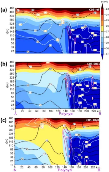
Figure 6.Surface temperature and 10 m wind field on 4 January 2008 at 15:00 UTC in(a)C05-ref (reference),(b)C05-50/1 (realistic), and (c)C05-10/0 (open water). In(d)anomalies (C05-10/0 minus C05-ref) over the AL polynya are shown for wind vectors (note different scale) and wind magnitude (colour shaded) at 10 m height and for pressure at mean sea level (green contour lines). The white line in(a)to(c) (magenta ind) marks the cross section A→B used for Fig. 7.
to be at the windward side now, which is owed to the TA and the thereby considered spatial thin-ice gradient. Another ef-fect, which becomes visible, is that the marginal area of the polynyas with warmerTsfcincreases with the use of TA. This effect is most obvious for the NET polynyas. This increases the area where heat is transferred from the ocean into the at-mosphere and causes smooth transitions from the fast or pack ice to the polynyas. An increased heat loss has to be balanced by an increase in frazil ice production.
5.1.2 10 m wind speed
The wind speed is the main driver for mixing in the ABL above polynyas and mainly controls the sensitive heat flux until the warming of the ABL reduces the vertical temper-ature gradient and thus the sensitive heat loss and subse-quently the ice production. Figure 6 shows the 10 m wind speed and direction on 4 January 2008 at 15:00 UTC. In the reference run (C05-ref) the wind speed above the AL polynya is about 14 to 18 m s−1. The wind speed slightly increases (Fig. 6d) in the sensitivity simulations (+2 to +5 m s−1).
This increase is caused by increased pressure gradients in the vicinity of the AL polynya which develop as the convec-tion above the polynya lowers the local surface pressure by
up to−0.5 hPa. Furthermore, the pressure anomaly is orien-tated alongside the polynya, resulting in slightly more anti-cyclonic wind directions. This increase of near-surface wind speed is in agreement with results from idealized studies con-ducted by Ebner et al. (2011) (see Fig. 5c therein). Ebner et al. (2011) concluded that the increase in wind speed re-sults in an increased net ice production, despite an increased boundary layer warming. The increase in near-surface wind speed causes a larger momentum flux (not shown, but see Sect. 5.1.3 for the TKE) and higher energy loss from the ocean. Furthermore, although not represented in the present CCLM model, higher wind speeds increase the sea-ice drift within polynyas, so that newly formed ice is likely to drift faster and a strong heat loss is maintained. Both processes are expected to increase the IP. However, the latter issue has to be investigated by coupled atmosphere–sea-ice–ocean model simulations.
5.1.3 Vertical cross sections
about −30◦C about the pack ice, and colder than−31◦C
over the fast ice. The boundary layer is stably stratified over the pack and the fast ice but over the polynya a well-mixed convective boundary layer (CBL) has developed, capped by an inversion at approximately 300 to 500 m height. Compar-ing the cross sections for the three shown model configura-tions, it becomes obvious that the assumptions on the thin ice within a polynya have considerable effects on the ABL.
As mentioned earlier, the onset of the CBL at the wind-ward polynya edge is displaced to the polynya interior in the reference simulation (C05-ref) compared to the sensitiv-ity simulations. This is due to the too thick ice in this area, preventing a large enough heat transfer and hence vertical mixing. This is also reflected in the low values of TKE com-pared to twice as high values for the sensitivity runs. In the open-water configuration (C05-10/0) the CBL is thus about 3◦C warmer than in the reference run. The warm air spreads
as a plume downstream the polynya and can be tracked sev-eral hundred kilometres over the pack ice (not shown).
One might suspect that the warmer CBL of the sensitiv-ity simulations might lead to a reduced vertical temperature gradient over the polynya and thus to a negative feedback for the surface sensible heat flux and thus ice production. This is not the case, since the surface temperature in areas with fractional ice cover is also warmer by about 6 to 16◦C, so
that the vertical gradient remains or even increases. Secondly, the wind speed in the sensitivity runs is increased over the polynya due to increased local pressure gradients and thus enhances the turbulent fluxes. The increased sensible heat flux causes also TKE production by buoyancy.
Almost all sensitivity simulations show considerably less cloud formation above and downstream the polynya com-pared to the reference simulation. Although the amount and location of clouds vary, the clouds almost vanish. The reason for this is that the maximum value of the specific humidity is about 0.4×10⁻³kg kg−1over the AL polynya in all sim-ulations, and if the CBL warms the condensation of water vapour is inhibited. As a result, nearly no clouds form above the polynya.
5.1.4 Total atmospheric energy flux
The above-mentioned findings result in an increased heat loss from the ocean, which is confirmed and shown in Fig. 8. In the reference simulation the total atmospheric heat flux (QA)
is, almost homogeneously, about−500 W m−2over the AL
polynya (note that the negative sign denotes upward fluxes). By assuming subgrid-scale open water the heat loss consid-erably increases, exceeding−1000 W m−2 at the windward edge and in the centre of the polynya. Higher and more struc-tured values ofQAresulted also from C05-50/1. The smooth
transition at the polynya margins is also visible from this fig-ure. Since we based the estimation of ice production on this quantity it is clear that there will be considerable differences as well.
Figure 7.Vertical cross sections of the potential temperature 2, horizontal wind speed (black contour lines), turbulent kinetic en-ergy (TKE in m2s−2, magenta contour lines), and cloud frac-tion (white contour lines and orange labels) on 4 January 2008 at 15:00 UTC for(a)C05-ref (reference),(b)C05-50/1 (realistic), and (c)C05-10/0 (open water). The horizontal distance is about 240 km and the location of the cross section A (pack ice)→B (fast ice) is shown in Fig. 2.
5.2 Energy balance components for the winter period 2007/2008
Figure 8.Total atmospheric energy flux on 4 January 2008 at 15:00 UTC in(a)C05-ref (reference),(b)C05-50/1 (realistic), and(c)C05-10/0 (open water). Negative fluxes are directed upwards. The white line marks the cross section A→B used for Fig. 7.
In principle, the processes presented in Sect. 5.1 come into effect whenever a polynya is present. Thus, if the tile approach is used, QA is always more negative due to the
consideration of subgrid-scale energy fluxes (Fig. 9) and more energy or heat is lost from the ocean. In the reference simulation (C05-ref) about −253 W m−2 is lost on average
within polynyas. If the subgrid-scale thin ice is reduced or replaced by open water then QA is much higher, reaching about−529 W m−2in the latter, which is about+110 %. In the simulation with a realistic configuration (C05-50/1) the increase is about+20 %, reaching about−303 W m−2on av-erage.
The largest contribution to QA constitutes the sensible
heat flux H (Fig. 9). About 66 % of the heat is lost viaH in the reference simulation, which slightly decreases to 57 to 65.6 % if the tile approach is used. The strongest impact on the sensible heat flux shows C05-10/0. Here,Hdoubles from 167 W m−2in C05-ref to
−325 W m−2due to the absence of
the isolating sea-ice cover. The increase is less in the other sensitivity simulations, e.g.+7.1 % in the case of C05-50/1. The other components contribute much less to the heat loss. However, the Bowen ratio (Bowen, 1926), which is the ratio H/E, reduces from about 4.0 ref) to 2.5 (C05-50/1) and 2.3 (C05-10/0). The latent heat flux (E) nearly
Figure 9.Temporal means of the energy balanceQAand its
Table 4.Total sea-ice production (IP) (km3) in the winter period 2007/2008, aggregated over polynyas within the four polynya masks (Fig. 2). The daily mean (x) and standard deviation (σ) are given in km3day−1. The Pearson correlation coefficient (r) was calculated with the IP time series and the estimates of Willmes et al. (2011a). The 95 % confidence interval (CI) ofrwas calculated based on the Fisher ztransformation. The critical value isrc,α=0.05,n=182=0.15 andris significant ifr > rc. Two-sidedttests (α=5 %) were performed and the resultingpvalues (p) are given. Significant differences are marked with∗. The results from Bauer et al. (2013) assumed an ice thickness of 10 cm (B10) or open water (B00) within polynyas, both without a tile approach.
Data Total x σ r[95 % CI] p
C05-ref 29.1 0.2 0.2 0.65[0.56; 0.73] 0.30
C05-10/10 29.2 0.2 0.3 0.63[0.53; 0.71] 0.34
C05-10/1 49.3 0.3 0.4 0.63[0.53; 0.71] 0.01∗
C05-10/0 65.2 0.4 0.6 0.61[0.51; 0.69] <0.01∗
C05-50/5 25.3 0.1 0.3 0.56[0.45; 0.65] 0.05∗
C05-50/1 38.3 0.2 0.3 0.60[0.50; 0.69] 0.30
Willmes et al. (2011a) 33.0 0.2 0.2 – –
MODIS2kma 49.1a 0.3a 0.4a 0.45[0.33; 0.56]a <0.01∗,b
B10 25.4 0.1 0.2 0.67[0.58; 0.74] 0.02∗
B00 45.5 0.3 0.4 0.68[0.59; 0.75] 0.03∗
aOnly for November–March;bcomparisons with Willmes et al. (2011a) were made only for
November–March.
0 1 2 3 4
km
3day
Nov Dec Jan Feb Mar Apr
C05-ref;(29.1km3)
C05−10/10;(29.2km3)
C05−10/1;(49.3km3)
C05−10/0;(65.2km3)
C05−50/5;(25.3km3)
C05−50/1;(38.3km3)
Willmes et al. (2011);(33.0km3)
MODIS (2km);(49.1km3)(Nov.−Mar.)
B10;(25.4km3)
B00;(45.5km3)
–1
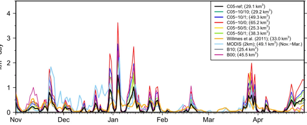
Figure 10.Daily sea-ice production within the Laptev Sea polynyas in the winter period 2007/2008, aggregated within the four polynya masks (only considering polynyas>277 km2in the C05 and Bauer et al., 2013, simulations – B10, B00). The total sea-ice production is given in parentheses in the legend (see also Table 4).
doubles for C05-50/1 compared to C05-ref, which is caused on one hand by the increase of the vertical gradient of spe-cific humidity and on the other hand by the increase of the near-surface wind speed and TKE, enhancing the turbulence above the polynyas. Shortwave radiationK∗ only becomes important in the time from March until April, when the melt-ing season begins. Therefore,K∗ is small compared to the other terms.
6 Effects on sea-ice production in the winter period 2007/2008
The daily sea-ice production rates were calculated for the in-dividual polynyas as described in Sect. 3.4. Here we com-pared the ice production of the C05 simulations to the re-mote sensing estimations of Willmes et al. (2011a), to
esti-mates based on MODIS2km (Sect. 3.4), and to model results of Bauer et al. (2013).
The time series of daily IP (km3day−1) are shown in
Fig. 10 and the total ice production for the whole winter are shown in Table 4. The total IP in the winter 2007/2008 is about 29.1 km3in the reference simulation (C05-ref), which is not significantly different from the 33.0 km3estimated by
Willmes et al. (2011a). The temporal correlation isr=0.65, which is sufficiently high, but some differences are visible (Fig. 10). This result agrees well with the remote sensing es-timates, although Willmes et al. (2011a) used a constantCH
for calculating the heat fluxes and much coarser atmospheric data.
as-Figure 11.Total sea-ice production (m) within the Laptev Sea polynyas in the winter period 2007/2008 simulated by(a)C05-ref (reference), (b)C05-50/1 (realistic), and(c)C05-10/0 (open water).
sumptions (C05-50/1) the IP increases to 38.3 km3(+39 %),
which is not significant at the 95 % level. The increase of IP is caused by the higher heat fluxes from the ocean into the overlying atmosphere as presented above. Compared to the results based on MODIS2km, where we estimated about 49.1 km3due to the large polynya area, most of the simula-tions produced much less ice. Excepsimula-tions are C05-10/0 and C05-10/1, which reach or even exceed this estimate. These results show that there are large differences not only between the models but also between remote sensing approaches. For instance, the time of polynya openings and IP also differ (r=0.45). Although such high IP could be reproduced in the Laptev Sea, the question remains of which remote sensing data set should be used for calibrating the models.
The IP based on an older reference COSMO simulation by Bauer et al. (2013) with 10 cm ice within polynyas (B10) is slightly less compared to our reference run (C05-ref), but significantly lower compared to Willmes et al. (2011a). Although the open-water sensitivity run of Bauer et al. (2013) (B00) produces higher IP, it is considerably less com-pared to our C05-10/0 run. B10 and B00 show a slightly higher correlation with the IP time series of Willmes et al. (2011a). The differences of B10/B00 with respect to our C05 simulations can be explained by differences in the model version, configuration, and nesting chain (GME vs.
ERA-Interim, different model domains). However, we cannot quantify the individual contributions to the deviations. All C05 sensitivity simulations show a higher daily standard de-viation compared to the data from Willmes et al. (2011a), which increases with decreasing subgrid-scale thin ice. This is logical, because if a polynya opens then more heat is re-leased compared to the reference simulation and thus the IP is higher.
7 Discussion
The simulation results of our study showed that there is a high sensitivity of the ice production to the assumptions on subgrid-scale thin-ice distribution, with considerable ef-fects on the atmospheric boundary layer. The ABL receives more heat the thinner the ice is and warmed by up to+3◦C in our subgrid-scale open-water configuration. However, the warmer ABL did not prevent further heat release from the ocean due to a weakened vertical temperature gradient. The simulations showed that the vertical temperature gradients remain or even exceed the gradients of the reference sim-ulations. Two effects are responsible for this: (i) as the ice becomes thinner the surface temperature increases stronger than the heating of the ABL, which increases the vertical gra-dient; and (ii) the near-surface wind speed is enhanced due to increased local pressure gradients, which increases the wind-shear and thus the sensible heat fluxes. Further, the warm plumes over the polynyas are efficiently advected over the pack ice. Thus heat is removed from above the polynyas and a strong temperature gradient is maintained, which enhances the ice production.
Constraining the assumptions on subgrid-scale thin ice was found to be difficult. The comparison of model-based IP with remote sensing estimates revealed large discrepancies. Further, large differences were found between the two remote sensing approaches. The usage of higher resolved MODIS data and ERA-Interim, compared to the approach of Willmes et al. (2011a) in which NCEP and AMSR-E data were used, nearly produced+50 % more ice. The configuration of C05-50/1, in which we assumed 50 cm thick grid-scale and 1 cm subgrid-scale thin ice, seems to be a realistic assumption in the marginal ice zone of the polynyas.
The resulting IP is close to the estimates of Willmes et al. (2011a), which we defined as a baseline for our sen-sitivity experiment. However, if for instance the results of MODIS2km were defined as a baseline, then even thinner ice might be considered. We are aware that our sea-ice module is simplified compared to more sophisticated sea-ice models, where the thin-ice thickness might be a prognostic variable and not a constant. However, despite our simple assumption, the results are promising and satisfactory in order to repre-sent sea ice in a regional climate model in a computationally cheap approach. We further argue, based on our results, that assuming subgrid-scale open water within fractional sea ice, such as in Polar-WRF (Bromwich et al., 2009), leads to too-high heat fluxes from the ocean into the atmosphere.
However, even if more sophisticated sea-ice models were used to estimate the IP, the issues remain of how to constrain parameters and to which data set to compare. It is not our in-tention to disentangle all factors controlling the estimation of sea-ice production based on different approaches, data sets, or models, but several issues are important in a general sense:
CH×103
P
(
CH
)
1.5 2.0 2.5 3.0 3.5
C05−ref
C05−10/10 C05−10/1 C05−10/0 C05−50/5 C05−50/1 MODIS 2 km
0 0.1 0.2 0.3 0.4 0.5 0.6
Willmes et al. (2011)
Figure 12. Probability density functions of the turbulent trans-fer coefficients for heat (CH) within the Laptev Sea polynyas in the winter period (November–April) 2007/2008, aggregated within the four polynya masks. The grey bars show the histogram of CH from C05-ref. Only values below 6×10⁻³ have been used for the construction of this figure. The mean values of the C05 simulations are ≈2.5×10⁻³ and the standard deviations are
≈0.28×10⁻³, except for C05-50/5 and C05-50/1 where the mean values are≈2.27×10⁻³and≈2.31×10⁻³, and the standard de-viations are ≈0.18×10⁻³, respectively. The constant value of CH=3.0×10⁻³of Willmes et al. (2011a) is marked with an arrow. The meanCHvalue derived from MODIS2km (November–March) isCH=2.3±0.3×10⁻³.
– Polynya area is affected by the definition of polynyas (e.g. SIC≤70 % orhi<0.2 m) and the horizontal
reso-lution of the model and the satellite products.
– Heat loss is affected by the vertical temperature gra-dient, wind speed, parameterization of the energy bal-ance components (turbulent fluxes), sea-ice thickness and properties, and the parameterization of the heat flux through the ice. Particularly important is the hor-izontal resolution of the atmospheric data set and the assumptions on the turbulent exchange coefficient for heat (CH). Willmes et al. (2011a) assumed a constant value of CH=3×10⁻³. However, the mean values
from C05 over polynyas (winter 2007/2008) are about (2.5±0.28)×10−3(Fig. 12), except for C05-50/5 and C05-50/1, which simulated slightly lower values of (2.27±0.18)×10−3and (2.31±0.18)×10−3.
– Since the warm surface temperatures of polynyas and the resulting vertical temperature gradients are not well represented in ERA-Interim or NCEP, the usage of a high value ofCH seems to partly compensate for this
issue. TheCH values based on MODIS data and
ERA-Interim are lower than simulated by CCLM with a mean of CH=(2.3±0.3)×10−3. A similar probability
hor-izontal resolution of MODIS, polynyas are represented as anomalies in the surface temperature field, causing larger vertical temperature gradients and henceCH val-ues, which are comparable to CCLM.
– Surface temperatures in remote sensing approaches also depend on the number of swaths per day, e.g. clear-sky conditions, and their distribution over the day. If not equally distributed, the surface temperature and the ice production may be biased.
These influence factors together control differences between model and remote sensing sea-ice production estimates within polynyas. The polynya area is an obvious factor with the simple relationship: the larger the polynya area, the larger the sea-ice production. Note that sea-ice grows also outside polynyas, which was simulated by our model and contributed to the total IP. However, compared to the contribution of the polynya areas to the total, the IP of such areas is of mi-nor importance. The explanations for differences in the heat or energy loss within polynyas is manifold. In our opinion, the most relevant factors, besides polynya area, are the thin-ice thickness and the parameterizations of the turbulent heat fluxes, in particular the differences inCH.
The complexity of these factors make a comparison of model and remote sensing studies difficult. It further in-dicates that some assumptions in the remote sensing ap-proaches, such as a constant value for CH, might be
over-simplified. Furthermore, a problematic issue is the usage of coarse atmospheric data sets, such as NCEP or ERA-Interim, for remote sensing approaches, if not combined with high-resolution satellite products. The horizontal high-resolution of such atmospheric reanalysis data sets is not sufficient to rep-resent polynyas adequately. Thus subsequent errors, such as wrong simulations of the atmospheric boundary layer over polynyas, are the consequence. These errors are then trans-ferred to the remote sensing approach and might result in wrong sea-ice production estimates. From a modelling point of view the question arises of what reference for IP estimates should be used. This question is not easily answered and is still an open issue. A strategy might be a simultaneous ap-plication of both modelling and remote sensing approaches in order to compensate for weaknesses. This issue directly impedes the decision of an optimal model configuration.
According to our study, the approach of Willmes et al. (2011a) constitutes the closest reference because of the same satellite data that were used to derive polynya area at a com-parable horizontal resolution. Although the definitions of polynyas are different, the assumption of 0.1 m thin ice in areas of SIC≤70 % is similar to the definition of≤0.2 m as in Willmes et al. (2011a). Larger differences evolve from the assumptions made on CH (Fig. 12) and the horizontal
res-olution of the atmospheric data. Given these deviations, the IP based on C05-ref and C05-50/1 is still close to the re-sults of Willmes et al. (2011a). Although the use of MODIS,
i.e. higher resolved satellite products, results in higher IP es-timates, the reason for this is the higher horizontal resolution that causes larger polynya areas and not the representation of subgrid-scale energy fluxes within polynyas in ERA-Interim, which is still too coarse. For thicker ice theCHvalues
con-verge to ≤1.5×10⁻³, a value also reported by Schröder et al. (2003).
Given these issues, the decision of which TIT should be used with the TA is another degree of freedom and cannot sufficiently be answered from our study. A justified assump-tion is to rely on MODIS TIT (Fig. 3). The mean derived TIT for the winter periods (November–March) 2002/2003– 2014/2015 is 13.5±0.5 cm, which is slightly thicker than our assumed TIT in CCLM. Unfortunately, the MODIS TIT dis-tribution for the polynya areas shows no maximum at a spe-cific ice thickness, which gives no preference for the choice of the subgrid TIT for the tile approach.
8 Conclusions
In this study we quantified the ice production in the Laptev Sea polynyas for the winter 2007/2008 based on simulations with a regional atmospheric model (CCLM) and remote sens-ing data. A new tile approach for fractional sea ice, consid-ering subgrid-scale thin ice, was implemented into CCLM. Besides a reference run, five sensitivity simulations with dif-ferent assumptions on grid-scale and subgrid-scale ice within polynyas were performed. We further investigated the impact on the atmospheric boundary layer above polynyas.
The results show that the ice production is highly sen-sitive to the assumptions made on the ice thickness within polynyas. Compared to the estimated total winter ice pro-duction of 29.1 km3of the reference simulation, the ice pro-duction more than doubled when subgrid-scale open water was assumed and increased by about (+39 %) for the most realistic assumptions based on remote sensing of ice thick-ness. The increase of the ice production is caused by a larger heat loss from the ocean, whose magnitude is proportional to the thin-ice thickness. Although the atmospheric bound-ary layer is heated by up to +3◦C in the open-water
In summary, realistic ice production estimates could be re-trieved from our simulations. Neglecting subgrid-scale en-ergy fluxes might considerably underestimate the ice produc-tion in coastal polynyas, such as in the Laptev Sea, with pos-sible consequence on the Arctic sea-ice budget.
9 Data availability
Appendix A: Sea-ice albedo scheme
We implemented a modified Køltzow scheme (Køltzow, 2007) (Fig. A1) to replace the default treatment of sea-ice albedo, which was previously set toαi=0.75 for ice
thick-ness>0.1 m andαi=0.2 for ice thickness≤0.1 m (Schröder
et al., 2011). Furthermore, the Køltzow scheme includes a pa-rameterization of melt ponds (see Køltzow, 2007, for details), yet they are of no importance for our study. The scheme is based on measurements retrieved during the Surface heat Budget of the Arctic Ocean (SHEBA) project (Uttal et al., 2002). It is forced by the surface temperatureTsfc, which may
be either the ice (Ti) or the snow surface temperature (Ts)
(Fig. 4). If no snow cover is present the albedo only depends on the ice thickness. If the ice thickness exceeds the thresh-old value ofhc=0.2 m, a snow cover on sea ice is assumed in accordance to the sea-ice module. Sea ice thicker thanhc is treated as thick ice and the albedo is estimated by
αi=
( 0.84 ifT
sfc≤ −2◦C 0.84−0.145(2+Tsfc) if 0◦C> Tsfc>−2◦C 0.51 ifTsfc>0◦C
. (A1) Køltzow (2007) sets the albedo for cold sea ice to a high value of 0.84, which is supposed to include the effects of snow on sea ice in winter and spring. In the original scheme Køltzow (2007) set the threshold for thin ice tohc=0.25 m,
but since the values above are only valid for snow-covered sea ice, we sethc=0.2 m to be consistent with the sea-ice
module.
For thin ice, we implemented a linear decrease towards the ocean albedo (αo=0.07):
αi=αo+(hi/hc)·(αc−αo) . (A2)
As a starting value we useαc=0.57, the albedo of thick bare
sea ice from Persson et al. (2002).
Figure A1 shows a summary of both cases. If the ice thick-ness is at least 0.2 m (bold black line) then the albedo is con-stant (αi=0.84) for cold, snow-covered sea ice. It decreases
with increasing surface temperature if −2◦C are exceeded.
This temperature denotes a threshold where melting begins and sea ice is changing its albedo characteristics. In addition, if melt ponds occur (black solid line), the albedo is some-what lower during the melting season. The fraction of melt ponds increases with Tsfc>−2◦C to a maximum of 22 %
(bold green line), an upper limit set by Køltzow (2007), and the albedo of melt ponds converges to the albedo of sea wa-ter (dashed green line). Furthermore, in Fig. A1 the thin-ice albedo is exemplified for four ice thicknesses which are not covered with snow and for which a constant albedo is as-sumed (thin black lines).
If the tile approach is used, subgrid-scale open water re-duces the grid-average albedo accordingly, compared to a complete coverage with sea ice. A comparable, though less pronounced, reduction of albedo occurs if 1 cm thin-ice cov-erage is assumed for subgrid-scale open water.
Tsfcin °C
Sea ice albedo
αi 0 0.1 0.2 0.3 0.4 0.5 0.6 0.7 0.8 0.9 1 0 0.1 0.2 0.3 0.4 0.5 0.6 0.7 0.8 0.9 1
−10 −5 −2 0 5
20 cm
Sea water 10 cm bare ice
5 cm bare ice
Cold sea ice Melting sea ice
Melt pond fraction
Snow co v er ed Ba re s e a i c e
No melt ponds
With melt ponds
Melt pond albedo 20 cm bare ice
Figure A1. Sea-ice albedo resulting from the modified Køltzow scheme (Køltzow, 2007) depending on the ice surface temperature and thickness. Thereby the threshold thickness above which a snow cover of 10 cm is assumed ishc=0.2 m (bold black line). In addi-tion the melt pond fracaddi-tion is shown as a funcaddi-tion of the ice tem-perature (bold green line) and the resulting modification (dashed green line) of the ice albedo (dashed black line). For bare sea-ice (thin black lines) a constant albedo value is assumed, which is linearly decreasing from 0.57 (Persson et al., 2002) at 20 cm ice thickness (bold grey line) to 0.07 (ocean albedo; Perovich and Gren-fell, 1981), but constant over all surface temperatures, as shown in Eq. (A2). The vertical blue lines mark the transition range from cold to melting conditions.
Appendix B: Implementation of the tile approach in CCLM
In order to simulate the subgrid-scale energy fluxes over frac-tional sea ice, it is necessary to differentiate the energy bal-ance and its components over water and ice. Over sea ice (in-dexk=i) or ocean (indexk=o) the total atmospheric heat flux (see Fig. 4) is
QA,k=Kk∗+L∗k+Hk+Ek, (B1)
withKk∗ the net shortwave radiation,L∗k the net longwave radiation,Hk the turbulent flux of sensible heat, andEk the
turbulent flux of latent heat.
All routines of CCLM, except the sea-ice and the turbu-lence module, calculate with grid-box averaged coefficients or fluxes (flux averaging approach; Vihma, 1995), which is best suited if the sea-ice module only requires the fluxes over ice (Lüpkes and Gryanik, 2015). The procedure is described in Sect. B3.
temperature of sea ice (Ti), specific humidity at the ice sur-face, the wind-speed on the lowest model level, and incoming longwave and shortwave radiation (see Schröder et al., 2011, for more details).
The calculation of the components of the energy balance equations are shown in the next subsections.
B1 Shortwave radiation
The grid-box average of the albedo αm (index “m” for
“mixed”) is calculated as
αm=A·αi+(1−A)·αo, (B2)
withAthe sea-ice fraction,αo=0.07 the albedo of the ocean, andαi=f (Ti,h)the albedo of sea ice as a function of sea-ice temperature (Ti) and thickness (h) (see Sect. A). Based on this mixed albedo the upward shortwave radiation is cal-culated as
K↑m=αm·K↓, (B3)
withK↓the incoming shortwave radiation. The grid-box av-eraged net shortwave radiation is calculated as
Km∗ =K↓ −K↑m=(1−αm)·K↓. (B4)
This grid-box averaged net shortwave radiation is the input for the sea-ice module where the upward shortwave radiation over iceK↑iis calculated as
K↑i=αi·K↓. (B5)
The final net shortwave radiation over sea ice or ocean be-comes
Kk∗=(1−αk)·K↓=
1−αk
1−αm·
Km∗, (B6) where the indexkrefers either toi(sea ice) oro(ocean). B2 Longwave radiation
The subgrid-scale ocean surface temperature (To) is assumed
to be at the freezing point (−1.7◦C) if open water is assumed,
or to be a prognostic variable if a thin-ice cover is assumed. The ice surface temperature (Ti) is also a prognostic variable
in the sea-ice module.
To account for subgrid-scale longwave radiation, we cal-culate the upward longwave radiation over sea ice and ocean as
L↑k=ǫσ Tk4−(1−ǫ)L↓, (B7)
with σ the Stefan–Boltzmann constant, L↓ the incoming longwave radiation, ǫ the surface emissivities of sea wa-ter and ice, which are assumed to be equal (ǫ=0.996), and Tkthe surface temperature of ice or ocean.
Then the net longwave radiation balance over sea ice or ocean becomes
L∗k=L↓ −L↑k. (B8)
B3 Turbulent fluxes of sensible and latent heat
We modified the parameterization of the turbulent fluxes of sensible (H) and latent heat (E) within a grid box, in contrast to the standard version of CCLM and the sea-ice module of Schröder et al. (2011). Over sea ice or ocean the roughness lengthz0and the turbulent coefficients of heat and moisture CHwere previously calculated from the predominant surface
type of a grid box: ice or sea water. We modified this proce-dure by a tile approach; now the fluxes are calculated both for sea ice and ocean within a grid box with differentz0andCH.
Afterwards they are averaged in a “flux-averaging approach” and an averageCHis calculated for other modules. The
cal-culation of the momentum flux is not modified and for the details of the calculation we refer the reader to Doms et al. (2011).
In CCLM a stability- and roughness-length-dependent sur-face flux formulation is used, which is based on flux calcu-lations after Louis (1979). The fluxes are calculated with a bulk approach:
H= −ρcpCH|vh|(2sfc−2) , (B9) E= −ρLfCH|vh|(qsfc−q) , (B10)
withρthe air density,cpthe heat capacity of air, and2and
2sfcthe potential temperature at the lowest model layer and
at the surface (ice or ocean).q andqsfc are the specific
hu-midity at the lowest model layer and at the surface (ice or ocean),Lfthe latent heat of fusion (and sublimation in case
of sea ice), |vh| = √
u2+v2 the absolute wind speed, and CHthe turbulent transfer coefficient for heat and moisture.
To calculate the turbulent transfer coefficients it is first necessary to calculate the roughness length of sea-water (z0,o) and sea ice (z0,i). In case of sea ice we set z0,i=0.001 m as in Schröder et al. (2011). Over open
wa-ter a modified Charnock formula is used (see Doms et al., 2011). In case ofH andE, we assume the additional rough-ness length for heatzh(Doms et al., 2011) to be equal toz0 over subgrid-scale open ocean within the sea-ice cover.
The transfer coefficients are calculated over sea ice (CH,i) and ocean (CH,o). The turbulent fluxes over sea ice (Hi,Ei)
and ocean (Ho,Eo) can be retrieved by inserting these
coef-ficients into Eqs. (B9)–(B10). Then all terms of Eq. (B1) are known to solve the energy balance over both surface types.
The fluxes of sensible and latent heat, the turbulent transfer coefficient for heat, and the surface temperature are averaged according to the sea-ice concentrationA: