Abstract— Satellite Communication Systems are beneficial in providing communication services to vast regions especially where the adequate infrastructure for communication may not be constructed. Wireless communication is one of the fastest growing fields in the engineering world. Introduction on adaptive antenna array is described in this paper. Linear adaptive algorithm LMS (Least mean square) is used to demonstrate the self-steering capability of an adaptive antenna array. It is done by changing number of elements in antenna array and angle of beam steering. The adaptive array has the ability to track the satellite automatically as it moves across the sky. MATLAB software has been used to obtain array voltage patterns for different values of number of elements in antenna array for different values of beam steering angle.
Index Terms—Satellite Communication, Adaptive antenna array, LMS Algorithm, Beam Steering
I. INTRODUCTION
Antennas are classified as either single element or array antennas (multi element). Single element antennas are either omni directional or directional. Omni directional antennas have equal gain in all directions and are also known as isotropic antennas. Directional antennas have maximum gain in desired directions and less in others.
Antenna array is an arrangement of many individual antennas which are placed in space and phase such that the contribution of individual antennas add in one desired direction and cancel in other directions. The antenna arrays are used to generate electronically steer able antenna patterns. The adaptive antenna array adjusts their pattern automatically to signal environment to reduce interference. The desired signal reception is maintained by steering the main beam. Spacing between array elements is an important factor in designing antenna arrays.
Antenna array may be phased array or adaptive array. A phased array antenna system is an array of omni directional ordirectionalelement antennas in which the signal induced on the antennas are combined to form an array output. Such an antenna system controls the direction where maximum gain appears by adjusting the phase difference between different antenna elements. An adaptive antenna array combines the outputs of antenna elements but controls the
Manuscript received December 28, 2007. This work was supported in part by the National Institute of Technology, Kurukshetra, Haryana..
Sangeeta Kamboj, Lecturer, A.P.J College of Engg Gurgaon, Haryana, phone: +91-9958639724; (e-mail: [email protected]).
Dr. Ratna Dahiya, Assistant Prof, N.I.T Kurukshetra, Haryana, phone: +91-9896848509; (e-mail: [email protected]).
directional gain of the antenna by adjusting both phase and amplitude of the signal at each individual element.
Satellite antenna consists of a parabolic reflector with horn antenna at its focus. Basically horn is used as feed for parabolic reflector. Usually Horn is placed at the focus of paraboloid.. The horn antenna have desirable property that it effects a smooth transition from medium like waveguide which supports finite number of propagating modes to a medium like free space which supports a infinite number of modes.[6] In most satellite communication systems, interference remains a problem for reliable reception of signals. Adaptive antenna array for satellite communication systems is better than omni directional antenna that radiate in all directions [4]. Hence for this we use adaptive antenna array that automatically steer the beam in the direction of desired signal i.e. signal of interest (SOI). An antenna array has same directional performance as that of larger antenna [1]. And radiation pattern is an important property of antenna. The overall radiation pattern of an antenna array is obtained by the radiation pattern of the individual elements, their positions, orientation in space and relative phase and amplitudes of the feeding currents to the elements [1]. Adaptive antenna arrays have ability to adapt changing environment conditions to maximize signal strength of signal of interest (SOI) [4]. In this paper MATLAB software has been used to obtain array voltage patterns for different values of number of elements in antenna array i.e. M and angle of beam steering i.e. x by using LMS algorithm.
II. ARRAY DESIGN ARCHITECTURE
The overall array pattern can be steered in direction of desired user without physically moving any of individual elements by varying amplitude and phase of individual elements output before combining [1]. The overall radiation pattern of an array is obtained by radiation pattern of individual elements, their positions, orientation in space and the relative amplitude and phase of feeding currents to the elements [1]. Figure ‘1’shows adaptive antenna array whose architecture is based on LMS algorithm [4]. It is shown in the figure that antenna array is a linear array in which centers of antenna elements are placed along straight line. Since the signals incident on all the antenna elements are of different phases due to the difference in distance traveled by the wave between two antenna elements.
The signal present at element one has traveled more distance )
sin(x
D than signal present at element two [1].Where D is distance between successive antenna phase centers in the array as shown in figure 1. Therefore phase of element one will lag behind that of element two by
β
D
sin(
x
)
[1].Where
Adaptive Antenna Array for Satellite
Communication Systems
Sangeeta Kamboj, and Dr. Ratna Dahiya,
Proceedings of the International MultiConference of Engineers and Computer Scientists 2008 Vol II IMECS 2008, 19-21 March, 2008, Hong Kong
β
(Phase propagation factor)=2
π
/
λ
Hereλ
=wavelength of received signal.In this figure1 the incident waves are defined as
s
(
t
)
. We will assume that the receiver will down convert the signal to its Intermediate Frequency(
IF
)
while the Analog-to-Digital converter(
A
/
D
)
will down convert the signal to its base band equivalent [4]. As they reach the antenna elements, the waves are converted to electrical signalsx
(
t
)
. From Figure1, we define the input signals asx
1(
t
),
x
2(
t
),...
.
x
n(
t
)
. These signals are then multiplied by the input weightsw
1,
w
2,...
w
n . Then output signaly
(
t
)
is the weighted sum of the input signals [4].
=
∑
n= ix
it
w
it
y
1
(
)
)
(
(1) Wheren
: Number of the weights.The error signal
e
(
k
)
in the following figure represents the difference between the summed output,y
(
k
)
and the reference signalr
(
k
)
. The error processor then computes the required weight adjustment necessary in order to null out the undesired signal. This process is an iterative process and will continue until all the weights in the array converge. Consider a narrow band incident wave as:)
2
exp(
)
(
t
=
A
π
f
t
+
φ
S
c (2)Where
A
: Amplitude of the signal. cf
: Carrier frequency.φ
: Phase difference between incidents waves at successive elements. i.e.φ =
2
π
/
λ
D
sin(
x
)
Fig. 1. An LMS adaptive antenna array
By taking received signal at element one as the reference, the received signals
x
i(
t
)
for uniform linear array with element spacingD
is represented in matrix form as [1].[
]
[
]
)
(
)
sin(
)
1
(
exp
.
.
.
)
sin(
exp
1
)
(
s
t
x
D
M
j
x
D
j
t
x
i⎥
⎥
⎥
⎥
⎥
⎥
⎥
⎥
⎦
⎤
⎢
⎢
⎢
⎢
⎢
⎢
⎢
⎢
⎣
⎡
−
−
−
=
β
β
(3))
(
)
(
)
(
t
a
x
s
t
x
i=
(4)Where
M
: Number of elements used in antenna array.x
: Angle of arrival w.r.t to y axis.)
(
x
a
: Steering vector which control direction of antenna beam.For adaptive beam forming, each element output
x
i(
t
)
is multiplied with weightw
ithat modify phase and amplitude relation between the branches and summed to give output)
(
t
y
[1].[
]
[
]
[
]
)
(
)
sin(
)
1
(
exp
.
.
.
)
sin(
exp
1
,...
,
)
(
1 2s
t
x
D
M
j
x
D
j
w
w
w
t
y
n⎥
⎥
⎥
⎥
⎥
⎥
⎥
⎥
⎦
⎤
⎢
⎢
⎢
⎢
⎢
⎢
⎢
⎢
⎣
⎡
−
−
−
=
β
β
(5))
(
)
(
t
w
x
t
y
=
i T (6) The overall antenna pattern is continuously modified by adjusting weight vector. For digital communication system, the input signals are in discrete time sampled data form [9]. Therefore output is:)
(
)
(
k
w
x
k
y
=
k T (7) Whereth
k
k
:
sampling instant.III. LMS ALGORITHM
A. Basic Description
The LMS algorithm was first introduced by Widrow et al [2] and operates with a priori knowledge of the direction of arrival and the spectrum of the signal but with no knowledge of the noise and interference in the channel. This algorithm is useful when the interference contains some spectral correlation with the SOI. Minimization of the MMSE can be accomplished by a gradient-search technique. The particular method that the LMS algorithm uses is known as the steepest decent technique. For this particular technique, the changes
Proceedings of the International MultiConference of Engineers and Computer Scientists 2008 Vol II IMECS 2008, 19-21 March, 2008, Hong Kong
in the weight vector are made along the direction of the estimated gradient vector.
The basic description of the LMS Algorithm is as follows [2]:
)
(
)
(
)
(
)
(
k
r
k
x
k
w
k
e
=
−
T(8)
)
(
)
(
2
)
(
)
1
(
k
w
k
e
k
x
k
w
+
=
+
μ
(9)Where
)
(
k
e
: Error signal between the reference signal and the desired output.)
(
k
w
: Weight vector before adaptation.)
1
(
k
+
w
: Weight vector after adaptation.μ
: Gain constant controlling rate of convergence and stability.Here we can see that the LMS algorithm does not require squaring, averaging or differentiating and hence can be implemented in most practical systems [2]. Its popularity is accredited to the fact that it is simple, easy to compute and efficient. However, the drawback is that the weights for this algorithm take a long time to converge.
B. The Convergence Rate of the LMS Algorithm
The parameter
μ
is the gain constant that regulates the speed and stability of adaptation. It determines the convergence rate. This gain factor is bounded by the limits 0<
μ
<
1/λ
maxWhere
max
λ
: Largest Eigen value of the input correlation matrix.IV. RESULTS
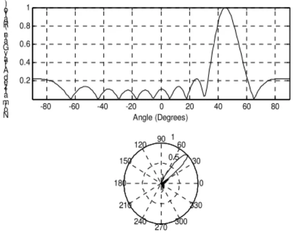
Figures 2, 3, 4 show array voltage patterns for different values of number of elements in antenna array (M) and angle of beam steering (x) as given in table I.
TABLE I
Beam Steering of LMS adaptive antenna array
S.No. Figure No. M x
1 2 5 30˚
2 3 8 45˚
3 4 15 60˚
The magnitude of the initial pattern is determined by the initial (arbitrary) choice of weights, w whereas the magnitude of the final pattern is determined by the strength of the desired signal, the direction and strength of the interfering signal and the noise in the system.
It is observed in figure 2, maximum gain occurs at an angle of 30˚ as angle of beam steering is fixed at 30˚. The figure 3 shows that main beam is at an angle of 45˚ because signal is received by the receiver at this angle In figure 4, the maximum gain occurs at an angle of 60˚ as angle of beam steering is fixed at 60˚
-80 -60 -40 -20 0 20 40 60 80
0.2 0.4 0.6 0.8 1
Angle (Degrees) No
r ma liz e d A rr a y Ga in ( Ra ti o)
0.5 1
30
210
60
240 90
270 120
300 150
330
180 0
Fig. 2 . Beam Steering of LMS adaptive antenna array having
x
=30˚;M
=5-80 -60 -40 -20 0 20 40 60 80
0.2 0.4 0.6 0.8 1
Angle (Degrees) No
r ma liz e d A rr a y Ga in ( Ra ti o)
0.5 1
30
210
60
240 90
270 120
300 150
330
180 0
Fig. 3. Beam Steering of LMS adaptive antenna array having
x
= 45˚;M
=8-80 -60 -40 -20 0 20 40 60 80
0.2 0.4 0.6 0.8 1
Angle (Degrees) No
r ma liz e d A rr a y Ga in ( Ra ti o)
0.5 1
30
210
60
240 90
270 120
300 150
330
180 0
Fig. 4 Beam Steering of LMS adaptive antenna array having
x
= 60˚;M
=15Proceedings of the International MultiConference of Engineers and Computer Scientists 2008 Vol II IMECS 2008, 19-21 March, 2008, Hong Kong
V. CONCLUSION
Linear adaptive algorithm LMS (Least mean square) may be used to demonstrate the self-steering capability of an adaptive antenna array. It can be easily done by changing number of elements in antenna array and angle of beam steering. It is confirmed by the above obtained results. Further it can be summarized that in satellite communication system, beam of adaptive antenna array by using LMS algorithm can be steered in direction of desired signal by changing number of elements in antenna array and angle of beam steering. It is proposed that maximum radiation may be received at an appropriate angle.
REFERENCES
[1] Donal F.Breslin, “Adaptive antenna array applied to position location” Master of science thesis, August1967, Virginia polytechnic institute and state university, Blacksburg.
[2] B. Widrow et. al. “Adaptive antenna systems,” Proc. IEEE, Vol. 55, No.12 Dec., 1967.
[3] Bernard Widrow, Samuel D.sterns, “Adaptive signal processing”,
Pearson Education Book Company, 2005.
[4] Keng Jin Lian, “Adaptive antenna arrays for satellite personal communication systems”, Master of science thesis, January 27,1997, Virginia polytechnic institute and state university, Blacksburg. [5] R.E. Collin. “Antennas and Radio wave Propagation”. McGraw-Hill
Book Company, 1985.
[6] Rajeswari Chatterjee, “Antenna theory and practice” New Age International Limited, Book Company, second edition 1996.
Proceedings of the International MultiConference of Engineers and Computer Scientists 2008 Vol II IMECS 2008, 19-21 March, 2008, Hong Kong