www.atmos-chem-phys.net/10/8803/2010/ doi:10.5194/acp-10-8803-2010
© Author(s) 2010. CC Attribution 3.0 License.
Chemistry
and Physics
Quantifying the contributions to stratospheric ozone changes from
ozone depleting substances and greenhouse gases
D. A. Plummer1, J. F. Scinocca1, T. G. Shepherd2, M. C. Reader1, and A. I. Jonsson2
1Canadian Centre for Climate Modelling and Analysis, Environment Canada, Victoria, BC, Canada 2Department of Physics, University of Toronto, Toronto, Canada
Received: 22 March 2010 – Published in Atmos. Chem. Phys. Discuss.: 15 April 2010 Revised: 1 September 2010 – Accepted: 6 September 2010 – Published: 20 September 2010
Abstract. A state-of-the-art chemistry climate model cou-pled to a three-dimensional ocean model is used to pro-duce three experiments, all seamlessly covering the period 1950–2100, forced by different combinations of long-lived Greenhouse Gases (GHGs) and Ozone Depleting Substances (ODSs). The experiments are designed to quantify the sepa-rate effects of GHGs and ODSs on the evolution of ozone, as well as the extent to which these effects are independent of each other, by alternately holding one set of these two forc-ings constant in combination with a third experiment where both ODSs and GHGs vary. We estimate that up to the year 2000 the net decrease in the column amount of ozone above 20 hPa is approximately 75% of the decrease that can be attributed to ODSs due to the offsetting effects of cool-ing by increased CO2. Over the 21st century, as ODSs
de-crease, continued cooling from CO2is projected to account
for more than 50% of the projected increase in ozone above 20 hPa. Changes in ozone below 20 hPa show a redistribu-tion of ozone from tropical to extra-tropical latitudes with an increase in the Brewer-Dobson circulation. In addition to a latitudinal redistribution of ozone, we find that the globally averaged column amount of ozone below 20 hPa decreases over the 21st century, which significantly mitigates the effect of upper stratospheric cooling on total column ozone. Anal-ysis by linear regression shows that the recovery of ozone from the effects of ODSs generally follows the decline in re-active chlorine and bromine levels, with the exception of the lower polar stratosphere where recovery of ozone in the sec-ond half of the 21st century is slower than would be indicated by the decline in reactive chlorine and bromine
concentra-Correspondence to:D. A. Plummer ([email protected])
tions. These results also reveal the degree to which GHG-related effects mute the chemical effects of N2O on ozone
in the standard future scenario used for the WMO Ozone Assessment. Increases in the residual circulation of the at-mosphere and chemical effects from CO2cooling more than
halve the increase in reactive nitrogen in the mid to upper stratosphere that results from the specified increase in N2O
between 1950 and 2100.
1 Introduction
Evidence can now be seen in the atmosphere for the efficacy of the controls on emissions of halogenated species enacted as part of the Montreal Protocol and subsequent amend-ments. The tropospheric concentrations of many of the pri-mary chlorine and bromine containing Ozone Depleting Sub-stances (ODSs) peaked in the early 1990s and have continued to decrease (Montzka et al., 1999; WMO, 2007), while the stratospheric concentration of reactive chlorine has peaked more recently (WMO, 2007). Projections show the contin-ued decrease of the atmospheric abundance of these species throughout the rest of the 21st century.
As the anthropogenic perturbation to halogen concentra-tions in the stratosphere decreases, other influences on the stratosphere can be expected to play a greater role. Foremost among these is the effect of climate change, driven largely by increasing concentrations of CO2. Increased concentrations
of CO2cool the stratosphere, with the effect maximizing near
the effect of temperature on chemical reaction rates (Haigh and Pyle, 1982; Brasseur and Hitchman, 1988), with the in-creased ozone acting to partly reverse the cooling (Jonsson et al., 2004). Cooling from increasing CO2over the recent past
is believed to have decreased ozone loss that would have oth-erwise occurred from ODSs by up to 20% in the upper strato-sphere (Rosenfield et al., 2005; Jonsson et al., 2009). Con-tinued future increases in CO2are projected to result in
up-per stratospheric ozone recovering more rapidly than would be expected from declining ODSs alone and eventually pro-ducing upper stratospheric ozone concentrations larger than those found in the past, before significant ODS perturbations (Rosenfield et al., 2002).
Changing climate can also be expected to affect strato-spheric ozone through changes to the residual circulation of the stratosphere. The Brewer-Dobson (B-D) circulation is driven by the dissipation of Rossby and gravity waves prop-agating upwards from the troposphere (e.g., Holton et al., 1995) and, as such, will be affected by changes in climate that modify the source and propagation of these waves. In fact, Chemistry-Climate Models (CCMs) have consistently shown an acceleration of the residual circulation as a result of climate change (Butchart et al., 2006), which can be ex-pected to affect the vertical and latitudinal distribution of ozone and other long-lived chemical species in the strato-sphere (Austin and Wilson, 2006; Shepherd, 2008; Waugh et al., 2009). However, it should be noted that there may be some discrepancy between model predictions of changes in the stratospheric circulation and estimated changes in age of air over the recent past inferred from the available observa-tions (Engel et al., 2009).
In addition to increasing CO2and climate change,
strato-spheric ozone may be affected by changing concentrations of other trace species. Reactions involving nitrogen ox-ides (NOx=NO+NO2) form the dominant ozone catalytic
loss cycles throughout much of the middle stratosphere. Therefore, changes in N2O, the source gas for stratospheric
NOx, can be expected to have important effects on
strato-spheric ozone (Chipperfield and Feng, 2003; Portmann and Solomon, 2007). Water vapour will also play a role – affect-ing the radiative balance of the stratosphere and, as a source of HOx (OH+HO2), playing an important role in ozone
chemistry, particularly in the upper stratosphere. The con-centration of stratospheric H2O may be affected by changes
to the tropospheric concentration of CH4 or the amount of
H2O entering the stratosphere through the “cold trap” around
the tropical tropopause (Austin et al., 2007; Oman et al., 2008).
Given the variety of commingled influences on the pro-jected future evolution of stratospheric ozone, attribution of changes in ozone to decreases in ODSs resulting from the Montreal Protocol is challenging. As seen from the discus-sion presented above, a great deal has been learned of how different factors may influence recovery of ozone. Some of these studies have used multiple linear regression of 3-D
Chemistry-Climate Model (CCM) results to apportion cause and effect (e.g., Jonsson et al., 2009; Oman et al., 2010). Other studies have used 2-D models to perform scenario simulations with different forcings alternately held constant or allowed to vary with time (e.g., Brasseur and Hitchman, 1988; Portmann and Solomon, 2007). Owing to their large computational cost, it is only more recently that full 3-D CCMs have begun to be used to investigate the influence of different factors through similar scenario simulations as used earlier in 2-D modelling studies (e.g., Waugh et al., 2009). However, these previous 3-D CCM scenario stud-ies merged separate simulations for the past (using observed Sea-Surface Temperature – SST – and sea ice fields) and fu-ture (modelled SST/sea ice) periods. Here we present three different scenario simulations, each based on an ensemble of three runs, performed with the Canadian Middle Atmosphere Model (CMAM) coupled to a 3-D interactive ocean and run continuously for 1950–2100 to explore the role of climate change and ODSs on the evolution of stratospheric ozone.
2 Model and experiments
The CMAM is built on the CCCma third generation atmo-spheric general circulation model (Scinocca et al., 2008). The model employs a spectral dynamical core with triangular truncation at total wavenumber 31 (T31) and 71 model levels in the vertical, with a lid at approximately 95 km for these simulations. The representation of stratospheric chemistry includes the important Ox, HOx, NOx, ClOxand BrOx
cat-alytic cycles controlling ozone in the stratosphere, as well as the chemistry of long-lived source gases such as CH4, N2O
and several halocarbons (de Grandpr´e et al., 1997). Chem-ical species, families or individual species where required, are advected using spectral advection. Heterogeneous reac-tions are included on sulphate aerosols, liquid ternary solu-tion (PSC type Ib) and water ice (PSC type II) particles. No sedimentation is allowed for these particles, with the material sequestered in the aerosol phase returning to the gas-phase when environmental conditions can no longer maintain equi-librium with the aerosol phase. Note that the model does not contain a parameterization of Nitric Acid Trihydrate (NAT) PSCs or associated denitrification.
2009), while particular aspects of the model have been tested in more targeted comparisons (e.g., Hegglin and Shepherd, 2007). Given the extensive assessment of CMAM performed previously, comparisons of CMAM with observations are limited here. For more information on the performance of CMAM as compared with observations the reader is referred to the articles mentioned above, the CCMVal report (SPARC CCMVal, 2010), as well as an upcoming special issue of CCMVal-2 papers in theJournal of Geophysical Research.
All of the simulations presented here were coupled to an Ocean General Circulation Model (OGCM) based on a modi-fied (Arora et al., 2009) version of the National Center for At-mospheric Research community ocean model (NCOM 1.3) (Gent et al., 1998). The OGCM employs the same land/sea mask as the atmospheric model and is specified to have nine ocean grid boxes within each atmospheric grid box, giving a horizontal resolution of approximately 1.9 degrees. The ocean model has 29 vertical levels with a 50 m upper layer and 300 m layers in the deep ocean.
2.1 Description of experiments
To explore the effects of long-lived Greenhouse Gases (GHGs) and ODSs on the evolution of strato-spheric ozone three different experiments were run, each with three ensemble members covering the period 1950– 2100. The first experiment follows the Chemistry Climate Model Validation (CCMVal-2) specifications for what is referred to as the REF-B2 experiment (Eyring et al., 2008) with time-evolving concentrations of GHGs and ODSs. The long-lived GHGs follow the moderate SRES A1B scenario (IPCC, 2000), with CO2 specified to increase to
700 ppmv by 2100, CH4peaking at 2.4 ppmv at mid-century
then declining to 2.0 ppmv and N2O increasing steadily to
370 ppbv at 2100. The specified lower boundary conditions for the halocarbons follow the A1 scenario (WMO, 2007), with a lower boundary condition for total organic chlorine increasing rapidly from 0.66 ppbv in 1950 to a peak of 3.6 ppbv in the early 1990s, then decreasing to 1.3 ppbv near 2100. Total organic bromine is specified to increase from 7.0 pptv in 1950 to 16.7 pptv in the late 1990s, then return to 8.3 pptv by 2100.
It is important to note that the radiation scheme in CMAM acts on only a single, prescribed, global average concentra-tion for each long-lived GHG, including CH4, N2O,
CFC-11 and CFC-12. The chemistry, on the other hand, acts on prognostic tracer concentrations, the spatial distribution of which reflects the effects of physical and chemical processes in the model and which may be forced at the surface by a prescribed concentration. While the specification of spatially uniform concentrations of long-lived GHGs in the radiation represents some inconsistency between radiative and chem-ical processes in the model, it also allows for the radiative and chemical effects to be easily separated by independently specifying the prescribed concentration passed to the
radi-ation and the prescribed boundary condition that forces the chemical tracers. This flexibility has been used for the sec-ond and third experiments described below.
In the second experiment, the concentration of the long-lived GHGs (including CFC-11 and CFC-12) passed to the radiation evolves following the same A1B scenario as the REF-B2 experiment. The lower boundary conditions for the halocarbon chemical tracers, however, are held constant at tropospheric concentrations for the year 1960. This experi-ment will be referred to below as the “GHG” simulation, to denote a simulation with evolving GHG forcing.
In the third experiment, the halocarbon chemical tracers are forced by the same time evolving tropospheric bound-ary condition as the REF-B2 experiment, while the specified GHG concentrations passed to the radiation are held at 1960 values. This experiment will be referred to as the “CHM” simulation below, as we use the results from this experiment to explore the effects of chemistry on the results, particularly the interaction of chemical processes with radiative forcing. Note that for the CHM simulation the concentrations of the chemical CH4 and N2O tracers are specified with a time
evolving lower boundary condition that is identical to that used in the REF-B2 experiment (SRES A1B scenario), while being held constant at 1960 concentrations for the radiation. Following the standard specification of climate change type simulations within the CCMVal activity, other external forcings were ignored. There are, therefore, no eruptive vol-canoes or solar cycle effects included in these simulations. All simulations were begun from an initial ocean state taken from an 1850 control run of the standard CCCma CGCM. To reduce computational cost and save time a single cou-pled simulation of dynamical CMAM, a version of the model without chemistry and using a specified ozone distribution, was run forward with evolving GHG concentrations to 1950. At 1950 a set of three simulations was launched using ran-domly perturbed atmospheric states. This first set of sim-ulations was found to be biased cold in the troposphere by approximately 0.5 K globally for present-day conditions and some minor model retuning was performed. The retuned ver-sion was used for the simulations presented here, with initial ocean states at 1950 taken from the year 2000 of the three initial simulations to provide a tropospheric climate repre-sentative of 1950. All simulations were begun in the year 1950 using the initial ocean state derived as described and the first ten years of the simulations were discarded, allowing some time for the chemical state of the atmosphere to “spin up”. To check whether this procedure might have introduced any transient artifacts, we examined the global average lower troposphere temperature over the period 1960–1979 in the constant GHG simulation (CHM) and could detect no trend, confirming the stable climate of the coupled system.
REF-(a) 1979-2000
-2.0 -1.5 -1.0 -0.5 0.0 0.5 1.0 Trend (K/decade) 1000
100 10 1
Pressure (hPa)
REF-B2 GHG (REF-B2 - GHG)
(b) 2010-2079
-2.0 -1.5 -1.0 -0.5 0.0 0.5 1.0 Trend (K/decade) 1000
100 10 1
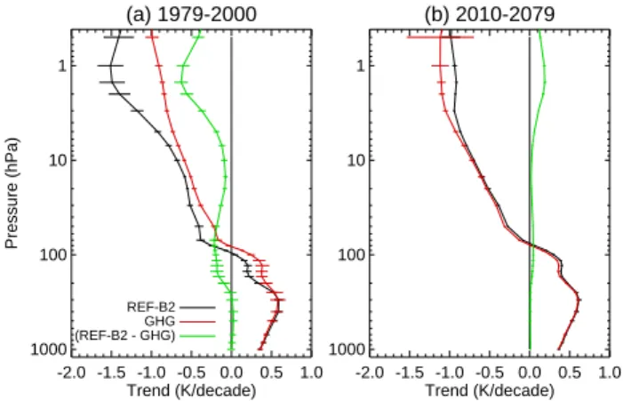
Fig. 1. Linear trends in global annual average temperature over the periods 1979–2000(a)and 2010–2079(b). Trends were calcu-lated from ensemble averages of the REF-B2 (black line) and GHG runs (red line). The trend attributed to ODSs, derived as (REF-B2– GHG), is given by the green line. The 95% confidence intervals of the trends are given by the horizontal bars.
B2 and the simulation with ODSs held constant at 1960 val-ues (the GHG simulation). The CHM simulation, with evolv-ing ODSs and constant radiative forcevolv-ing, is explored sepa-rately for the effects of long-term changes in the B-D circu-lation and CO2cooling on the chemistry of the stratosphere.
Note that the set of scenario runs analyzed have been sub-mitted to the CCMVal-2 model intercomparison and form part of the multi-model ensemble of scenario runs presented in Eyring et al. (2010).
3 Results
We begin with vertical profiles of trends in the global-average temperature from the different experiments shown in Fig. 1. The trends are presented for two time periods; for 1979– 2000, when the concentration of ODSs was rising rapidly, and for the period 2010–2079 during which the concentration of ODSs was more slowly decreasing. The trends are calcu-lated using least-squares estimation based on annual average temperatures of the ensemble mean of each experiment. The 95% confidence interval of the trend, accounting for auto-correlation in the time series using the “adjusted standard er-ror” method of Santer et al. (2000), is given by the horizontal bars on each vertical profile. The effects of ODSs on temper-ature are calculated by creating an annual time series of the differences between the ensemble means of the REF-B2 and GHG simulations and calculating trends from this data.
First, we note that the temperature trends of the REF-B2 and GHG runs are statistically identical through much of the troposphere for both time periods. This is as expected, since the radiative forcing from the long-lived GHGs for these two runs was constructed to be identical. Differences are found in the 1979–2000 global average trends between 200 and
100 hPa, reflecting the effects of stratospheric ozone deple-tion on temperature in the lowermost extra-tropical strato-sphere in the REF-B2 runs. Above the tropopause, given that globally averaged the stratosphere is close to radiative equilibrium, the global temperature trends shown in Fig. 1 largely reflect the effects of changing concentrations of ra-diatively active species. For the 1979–2000 time period the REF-B2 simulation reproduces the main features of the ob-served temperature trends over the recent past, with negative temperature trends throughout the stratosphere generally in-creasing with height and a maximum cooling of 1.5 K/decade around the stratopause (Randel et al., 2009). We note that the REF-B2 cooling trends for the recent past presented here are slightly larger than those shown for CMAM in Eyring et al. (2007), particularly through the mid- to upper-stratosphere, as an interpolation error in the CO2cooling parameterization
has been recently corrected (Jonsson et al., 2009).
The effect of ODSs on temperature is given by the trend in the difference (REF-B2–GHG) and is shown by the green line in Fig. 1. For the 1979–2000 period shown in panel a, the effect of ODSs on temperature is large in the lower strato-sphere, comes to a minimum around 10 to 20 hPa, then in-creases in the upper stratosphere. This pattern in the vertical distribution of differences in the temperature trends is a re-flection of the differences in ozone changes between these two runs (see below) and approximates the expected pattern of halogen-driven ozone loss (e.g., WMO, 2007). Further, we find that temperature trends in the REF-B2 and GHG ex-periments are statistically identical in the tropics (22◦
S to 22◦N) at all levels below 20 hPa (not shown), showing that
the effects of ODSs on global average temperature trends in the lower to mid-stratosphere are due to ozone changes at extra-tropical latitudes. This is a reflection of the fact that halogens play a relatively minor role in the chemistry of the tropical lower to mid stratosphere.
Cooling in the upper stratosphere is largely a result of decreases in ozone, decreasing the shortwave heating by ozone, and increases in longwave cooling from increasing CO2(Shine et al., 2003). Comparing temperature trends of
the REF-B2 and GHG simulations, we find that for the 1979– 2000 period CO2, with a small additional contribution from
increasing H2O, contributes a minimum of 60% of the total
cooling found in REF-B2 at the stratopause, with larger con-tributions above and below. The CO2contribution to cooling
defined in this manner implicitly includes a reduction of the cooling by the response of ozone to lower temperatures in this region. Following the argument of Shepherd and Jonsson (2008) that ozone is an internal property of the atmosphere, the cooling rate from CO2defined in this manner would then
be the most accurate estimate of the total effect of CO2on
mitiga-(a) REF−B2 to 1990−2009 (%)
−90 −60 −30 0 30 60 90
Latitude 100 10 1 Pressure (hPa) −16−12 −12 −8 −8 −8 −8 −6 −6 −6 −4 −4 −2 −2 0
2468 12 1620
(b) GHG to 1990−2009 (%)
−90 −60 −30 0 30 60 90
Latitude 100 10 1 −8 −6 −4 −2 0 0 2 2 2 4 4 6 8
(c) (REF−B2 − GHG) to 1990−2009 (%)
−90 −60 −30 0 30 60 90
Latitude 100 10 1 −16−12 −12 −8 −8 −6 −6 −4−2 −2
0 2 4 6 8
(d) REF−B2 to 2080−2099 (%)
−90 −60 −30 0 30 60 90
Latitude 100
10 1
Pressure (hPa) −20−16
−12 −8−6 −4−2 0 0 2 2 2 4 4 4 6 6 6 8 8 12 12 12 16 16 16 16 20 20 20 25 25
(e) GHG to 2080−2099 (%)
−90 −60 −30 0 30 60 90
Latitude 100 10 1 −20−16 −12 −8 −8 −6 −6 −4 −4 −2 −2 0 0 0 2 2 2 4 4 4 6 6 6 6 8 8 8 8 12 12 12 12 16 16 16
202530
(f) (REF−B2 − GHG) to 2080−2099 (%)
−90 −60 −30 0 30 60 90
Latitude 100
10 1
−6 −4−20 0 2 2 4 4 6 6 6 8 8 8 12 12 12 16
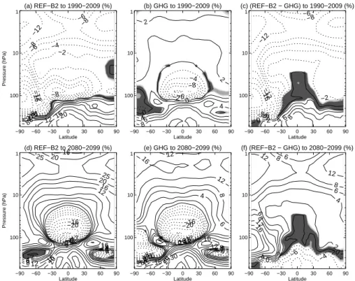
Fig. 2.The change in the zonal annual average ozone mixing ratio from 1960–1974 to 1990–2009 (top row) and the change from 1990–2009 to 2080–2099 (bottom row) for REF-B2, GHG and (REF-B2–GHG). All changes are expressed as percentages of the 1960–1974 average. Shading denotes regions where the differences are not statistically significant at the 98, 95 and 90% level as deduced from the student’s t-test accounting for lag-1 autocorrelation.
tion of the cooling from ODSs due to the internal response of ozone to additional cooling.
These results are broadly in agreement with previous es-timates of the relative contribution of ozone depletion and CO2 cooling to the upper stratospheric temperature trends
(Shine et al., 2003; Jonsson et al., 2009). The exact con-tribution assigned to ODSs will be sensitive to the magni-tude of ozone depletion in the model, though the decrease of ozone in these CMAM REF-B2 experiments is roughly in agreement with observations in the mid to upper stratosphere (Jonsson et al., 2009). We further note that these results are sensitive to the exact period over which the trends are calcu-lated, with the ODS contribution approaching 50% at 1.5 hPa when the trends are calculated over 1975–1995, for example, avoiding the late 1990s when the rate of increase of halogens in the upper stratosphere slowed markedly.
Temperature trends for the future period (panel b) show the dominant effect of increasing concentrations of CO2through
the 21st century. The recovery of ozone from halogens will take place at a much slower rate than the rapid depletion that occurred between 1980 and 2000 (e.g., Eyring et al., 2007) and we find that global temperature trends attributed to ozone recovery from ODSs are correspondingly smaller. For the period 2010–2079, temperature trends in the REF-B2 sim-ulation are very similar to those in the GHG runs, where
halocarbon concentrations were held constant at 1960 lev-els. The results show a small warming trend due to ozone increases from decreasing halogens in the lower stratosphere and a larger trend from approximately 5 to 1 hPa in the upper stratosphere.
3.1 Ozone changes: recent past
Changes of ozone in the recent past, during the period when stratospheric halogen concentrations were rapidly increas-ing, and during the period to the end of the 21st century over which ODSs are projected to more slowly decrease, are pre-sented in Fig. 2. Panels a–c of Fig. 2 present zonal cross-sections of the absolute change in the annual average ozone mixing ratio between the periods 1960–1974 and 1990–2009 for the REF-B2 and GHG simulations and, as above, the change attributed to ODSs derived from the difference be-tween the two simulations. The bottom three panels present a similar set of plots for changes between the periods 1990– 2009 and 2080–2099. All changes are expressed as a per-centage of the 1960–1974 average, when the REF-B2 and GHG experiments gave statistically identical distributions of ozone, so that changes can be compared between experi-ments and between time periods.
strato-sphere, with maximum losses toward the higher latitudes in each hemisphere, and a much smaller decrease in the mid-stratosphere, generally reproducing the pattern of observed changes in ozone over the recent past (Randel and Wu, 2007). These simulations also show the large observed decreases in the Southern Hemisphere lower stratosphere associated with PSC chemistry and Antarctic ozone depletion. We note one area of disagreement with observations over high latitudes in the Northern Hemisphere lower stratosphere. In this region observations show net changes of−4 to−8% from 1979 to
2005 between 50 and 200 hPa (Randel and Wu, 2007), while CMAM shows decreases of no more than 2% with statisti-cally significant increases below 150 hPa. As noted above, CMAM does not contain a parameterization of NAT or den-itrification and this may be contributing to the underestima-tion of ozone loss in this region. However, the exact role of NAT in polar heterogeneous chemistry is still uncertain (Drdla et al., 2002) and there remains no clear consensus on how best to parameterize NAT in models (WMO, 2007, Sect. 4.2.2), particularly given the computational constraints of CCMs. Decadal-scale dynamical variability may also have contributed to producing larger apparent trends in the obser-vations, particularly at levels below 18 km (∼65 hPa) (Yang
et al., 2006; WMO, 2007, Sect. 3.2.3.2). It is notable, in this respect, that most CCMs examined by CCMVal underpredict the observed Arctic ozone loss by roughly a factor of two (SPARC CCMVal, 2010, chapter 9), lending additional cre-dence to this hypothesis.
Between 1960–1974 and 1990–2009, the REF-B2 simu-lation produces decreases in ozone across the upper strato-sphere of 6 to more than 12% due, predominantly, to the combined effects of increasing halogens partly offset by cooling, while the GHG simulation with constant concen-trations of ODSs produces an increase in ozone of 2 to 3%. As before with temperature trends, we estimate the effects of ODSs on ozone by the difference between the REF-B2 and GHG experiments, shown in panel c of Fig. 2. The net change in ozone in the REF-B2 experiment is between 65% (around 10 hPa) and 85% (around 1 hPa) of the change that can be attributed to ODSs (not shown). The decrease in the apparent effect of ODSs on ozone in the REF-B2 simulation is due to increases in ozone due to cooling by CO2, with the
magnitude of the effect derived here being roughly in accord with the results from multiple linear regression analysis by Jonsson et al. (2009).
In the tropical lower stratosphere, both the REF-B2 and GHG simulations produce significant decreases in the con-centration of ozone. An increase in tropical upwelling is one aspect of the response of the B-D circulation to cli-mate change and is almost unanimously projected to occur by CCMs (Butchart et al., 2006, 2010). The more rapid tropical upwelling results in a decrease in the transport time of ozone-poor air from the troposphere, resulting in decreased ozone concentrations in the lower tropical stratosphere (Waugh et al., 2009; Eyring et al., 2010). The change in ozone found in
the model simulations is qualitatively similar to trends seen in observations (Randel and Wu, 2007), though the compari-son must be approached with caution. As discussed by Ran-del and Wu (2007) there remain a number of caveats to the observations of ozone in the lower tropical stratosphere in-cluding relatively low ozone concentrations and strong verti-cal gradients that make satellite observations difficult and the fact the SAGE satellite observations are in geometric height coordinates and may then be affected by geopotential height trends due to tropospheric warming. Further, the observed trends in the zonal mean ozone concentration would also im-ply decreasing trends in total column ozone, something that is not apparent in the independent observations of total col-umn, unless there are compensating increases in tropospheric ozone (Randel and Wu, 2007).
Although both the REF-B2 and GHG simulations display similar decreases in ozone in the tropical lower stratosphere related to changes in tropical upwelling, there are notable differences in the Southern Hemisphere that show the effect of ODS-driven ozone depletion at higher latitudes reaching to tropical latitudes. The GHG simulation shows decreases in ozone that extend across almost all latitudes where the residual vertical velocity is positive (approximately 35◦
S to 35◦
N) in the lower stratosphere, with decreases that are ap-proximately symmetric around the equator. The decrease in ozone in the REF-B2 run displays a local maximum around 20◦
S that results from the equator-ward mixing of ozone de-pleted air from higher latitudes. The pattern of the differ-ences can be seen more clearly in the (REF-B2–GHG) dif-ference, shown in panel c. Decreases of ozone of 2 to 4% are found at 70 hPa between 20 and 30◦S, while in the
North-ern Hemisphere at these latitudes changes in ozone are not statistically significant.
Both the REF-B2 and GHG simulations show significant positive trends in ozone in the troposphere, though these changes must be viewed with caution. These increases are likely related to increases in stratosphere-to-troposphere ex-change of ozone with ex-changes in the B-D circulation (Heg-glin and Shepherd, 2009). However, the version of CMAM used for these experiments does not calculate chemistry on model levels below 400 hPa and does not contain parameter-izations of processes such as ozone precursor emissions or wet deposition or other processes important for tropospheric chemistry and therefore, the magnitude of the response of ozone in the troposphere is likely incorrect.
3.2 Ozone changes: future
We now focus on changes from 1990–2009, the period en-compassing the peak ODS concentrations, to the end of the 21st century shown in the lower panels of Figure 2. While cooling from CO2 had only a small effect on ozone in the
upper stratosphere up to 1990–2009, cooling from increas-ing CO2becomes an important effect driving ozone increases
More than 50% of the increase in ozone above 10 hPa found in the REF-B2 run between 1990–2009 and 2080–2099 can be attributed to cooling from CO2, consistent with what was
inferred by linear regression in Jonsson et al. (2009). The contribution from ODSs (panel f) is, as would be expected from the temporal evolution of the concentration of ODSs, largely a reversal of the decreases found between 1960–1974 and 1990–2009 shown in panel c. The tropospheric concen-tration of halocarbons specified for 2080–2099 is similar to that specified for the early 1970s, therefore not all of the de-creases in ozone attributed to ODSs from the 1960–1974 ref-erence period have been recovered by 2080–2099. However, with the additional contribution from CO2 cooling, ozone
above 10 hPa in the REF-B2 run is from 5 to 15% higher in 2080–2099 than the 1960–1974 average.
Throughout the 21st century ozone concentrations in the low latitudes of the lower stratosphere decrease, reflecting the long-term increase in tropical upwelling and a decrease in the time for photochemical ozone production as tropospheric air enters the stratosphere. Maximum decreases of more than 40% are found in ozone between 1960–1974 and 2080–2099 around 80 hPa in both the REF-B2 and GHG simulations (not shown directly, but the sum of changes shown in panels a and d for REF-B2). The CMAM results are not unique, as al-most all of the CCMs that participated in CCMVal-1 and pro-vided results to 2050 displayed a similar decrease in ozone in the lower tropical stratosphere by 2050 (Eyring et al., 2007). While many CCMs project a qualitatively similar response of ozone in the lower tropical stratosphere, the magnitude of the response shown by CMAM should be placed in con-text relative to other CCMs. The annual average tropical up-welling mass flux in these REF-B2 simulations is approxi-mately 8.5×10⁹kg/s at 70 hPa for the year 2000, which is larger than that produced by many of the CCMVal-1 CCM simulations shown in Butchart et al. (2010). More relevant for changes in ozone, the rate of increase of tropical up-welling at 70 hPa in CMAM is found to be 2.0×10⁷kg/s/year (2.4%/decade) in the REF-B2 simulations, also at the upper end of estimates from the different CCMs in Butchart et al. (2010). That changes in tropical upwelling are towards the upper end of estimates from different CCMs implies that the trends in tropical ozone shown here are likely towards the upper end of CCM estimates (see also section 9.3.5, SPARC CCMVal (2010)).
We note that the upwelling mass flux is approximately 10% larger, and the rate of increase of tropical upwelling 60% larger, in these simulations than in those given by CMAM in previous simulations using specified SSTs for CCMVal-1. The origins of the changes in the residual cir-culation are not known at this time, but may be related to changes in the tropospheric climate as a result of parameter tuning to achieve radiative balance for coupling to the ocean model.
At higher latitudes in the lower stratosphere, the response of ozone to climate change alone (the GHG experiment in
panel e of Fig. 2) shows an asymmetrical response between the hemispheres, with increases between 80 and 200 hPa in the Northern Hemisphere and decreases in the lower strato-sphere at high southern latitudes. These changes in ozone follow changes in the residual circulation. As discussed by McLandress and Shepherd (2009), the CMAM response to climate change is to produce an increase in downwelling over the pole in the Northern Hemisphere and a decrease in downwelling over the southern polar cap. For the Northern Hemisphere the increased downwelling produces increases in ozone of between 6 and 15% in the lowermost stratosphere in the annual average. The absolute change in the ozone mix-ing ratio from 1990–2009 to 2080–2099 in this region max-imizes in early spring (February-March-April) and reaches a minimum in late fall, consistent with an increase in the dy-namical buildup of ozone over the winter. The response of the GHG run at high latitudes in the Southern Hemisphere is opposite of that found in the Northern Hemisphere, consis-tent with the decreased downwelling in the future. Although the seasonal cycle of ozone in the lowermost stratosphere over Antarctica is not as pronounced as over the north polar cap, the largest changes in the GHG run occur similarly in spring with decreases in 2080–2099 maximizing in October-November. Note as well, the GHG run shows a decrease in ozone centered around 250 hPa and poleward of 50◦
N that is associated with a decrease in the tropopause pressure with climate change (Son et al., 2009). A similar feature is evident in the Southern Hemisphere, though isolating the effects on ozone is more difficult given the general decreases of ozone in the lower stratosphere.
Changes in lower stratospheric ozone also show the effects of the steady decrease in halogen concentrations over the 21st century. The effect of ODSs on ozone between 1990– 2009 and 2080–2099, derived as the difference between the REF-B2 and GHG simulation and shown in panel f, is largely a reversal of the changes between 1960–1974 and 1990– 2009. Increases in annual mean ozone of more than 20% at high southern latitudes are attributed to ODSs, with changes in the annual mean driven by increases in ozone of more than 50% in October–November (not shown). Smaller in-creases attributed to ODSs are also found in the Northern Hemisphere mid and high latitudes. It is noteworthy that over 2080–2099 average ozone in the REF-B2 and GHG simula-tions are statistically identical below about 10 hPa, except for a region poleward of 60◦
S, and extending down to 150 hPa, where the REF-B2 run is from 2–4% lower than the GHG run (not shown).
3.3 The role of ODSs
(a)
-90 -60 -30 0 30 60 90
Latitude 100
10 1
Pressure (hPa)
0.10 0.10
0.20
0.20
0.20
0.40
0.40
0.40 0.60
0.60
0.60
0.80
0.80 0.90
0.90
0.90
0.95
0.95 0.95
0.98
0.98
(b) 16˚S - 16˚N at 5 hPa
1960 1980 2000 2020 2040 2060 2080 2100 Year
7.0 7.5 8.0 8.5 9.0 9.5
O3
VMR (ppmv)
-0.5 0.0 0.5
Difference (ppmv)
R2= 0.97
(c) 16˚S - 16˚N at 20 hPa
1960 1980 2000 2020 2040 2060 2080 2100 Year
6.6 6.8 7.0 7.2 7.4 7.6
O3
VMR (ppmv)
-0.2 -0.1 0.0 0.1 0.2 0.3
Difference (ppmv)
R2
= 0.82
(d) 60 - 90˚S at 50 hPa
1960 1980 2000 2020 2040 2060 2080 2100 Year
2.0 2.5 3.0 3.5
O3
VMR (ppmv)
-0.6 -0.4 -0.2 -0.0 0.2 0.4
Difference (ppmv)
R2
= 0.95
(e) 60 - 90˚N at 80 hPa
1960 1980 2000 2020 2040 2060 2080 2100 Year
1.6 1.8 2.0 2.2 2.4
O3
VMR (ppmv)
-0.2 -0.1 0.0 0.1 0.2
Difference (ppmv)
R2
= 0.55
Fig. 3.(a)presents the coefficient of determination from the fit of the smoothed (REF-B2–GHG) ozone timeseries to EESC. Shading denotes regions where the difference between the REF-B2 and GHG runs for 1990–2009 average ozone was not statistically significant at the 95% level. (b) through (e) present timeseries of the ensemble average ozone mixing ratio from the REF-B2 (black line) and GHG (red line) runs averaged over 16◦S–16◦N at 5 hPa(b), 16◦S–16◦N at 20 hPa(c), 60–90◦S at 50 hPa(d)and 60–90◦N at 80 hPa(e).
The orange solid line is the difference (REF-B2–GHG) in ozone and the blue dashed line the result of fitting the difference to the local EESC timeseries. All ozone timeseries display both the original annual averages (thin line) and the series after smoothing with a Gaussian filter with a width of 4 years (thick line).
(REF-B2–GHG) of the monthly and zonally averaged ozone mixing ratio and timeseries of the zonally and monthly av-eraged Equivalent Effective Stratosphere Chlorine (EESC) have been constructed. Following WMO (2007), EESC is defined as
EESC=Cly+60Bry (1)
though here [Cly] and [Bry] are the model calculated
con-centrations of total inorganic chlorine and bromine, respec-tively (note that while no single value ofα, the coefficient
on [Bry], is appropriate throughout the stratosphere, we have
performed the following analysis with values ofαof 5 and
60 and found the results to be very similar). Both time-series have been smoothed with a Gaussian filter with a width of 4 years to remove the annual cycle and some of the higher frequency inter-annual variability, and the first and last 10 years of the timeseries were dropped from the analysis to avoid periods where the filter is not fully immersed in the data. The resulting, smoothed (REF-B2–GHG) ozone time-series for 1970–2089 was then regressed on to the smoothed
EESC timeseries. The coefficient of determination of the re-gression (R2) is shown in Fig. 3a and, to delineate regions
where ODSs have only small effects on ozone, shading has been added to show regions where the 1990–2010 average ozone in the REF-B2 and GHG runs is not statistically dif-ferent at the 95% confidence interval. We find that the time-series of EESC can account for more than 80% of the vari-ance (R2>0.8) in the (REF-B2–GHG) ozone timeseries for
the period 1970–2090 over a large part of the atmosphere. The constructed EESC timeseries fits the (REF-B2–GHG) ozone particularly well for the mid to upper stratosphere, where the photochemical lifetime of ozone is short, and over a large part of the Southern Hemisphere stratosphere where the effects of Antarctic ozone depletion are large. TheR2
below approximately 70 hPa, where values of R2 are less
than 0.6. It should be noted that the exact values ofR2are
somewhat subjective, in that they depend on the amount of smoothing applied to the ozone timeseries that acts to reduce the contribution of interannual variability to the variance. Us-ing unsmoothed annual averages of the ensemble mean di-rectly yieldR2values of greater than 0.8 above 10 hPa and
in the Southern Hemisphere lower stratosphere, with values of 0.4 to 0.6 in the Northern Hemisphere middle stratosphere. Here, as we are focusing on the long-term evolution of ozone, theR2values from the smoothed timeseries are preferred.
More details of the EESC fit can be seen in panels b–e of Fig. 3, which present both the original and smoothed time-series of ozone along with the derived EESC fit for particular regions. In the upper stratosphere the interannual variability is small relative to the ODS perturbation andR2values are
quite large, while at high latitudes in the lower stratosphere the interannual variability, even with smoothing, is larger and contributes to variability that cannot be accounted for by the EESC fit and yields lower values ofR2. In general,
how-ever, one can see that the EESC fitting largely follows the long-term evolution of the (REF-B2–GHG) ozone difference – results that are similar to those of Waugh et al. (2009).
Closer inspection of the EESC fit to the (REF-B2–GHG) ozone at high southern latitudes (Fig. 3d) suggests some ten-dency of the ozone difference to fall below the EESC fit in the latter half of the 21st century. To analyse how well the EESC fit follows the evolution of ozone in the future, the av-erage residual of the ozone-EESC fit has been calculated for the period 2060–2089 and is shown in Fig. 4 expressed as a percentage of the 2060–2089 average ozone. By definition, the residuals to a least-squares fit should average to zero and we find that is the case over the entire 1970–2089 period for all points (not shown). As can be seen in Fig. 4, we find this also generally holds true over the shorter 2060–2089 pe-riod where, accounting for variability, the residuals are not statistically different from zero at even the 90% confidence level. We do find, however, two regions where the residuals are non-zero. Over the southern polar cap, south of 60◦
S and below approximately 40 hPa, the residuals are non-zero at the 98% confidence level and the EESC fit overestimates ozone by 1 to 3%. A second area in the upper stratosphere, centered around 55◦
S and 4 hPa, has average residuals that are non-zero at the 95% confidence level with the EESC fit underestimating ozone by approximately 0.25%.
The analysis of the residuals of the ozone-EESC fit sug-gests that ozone in the Southern Hemisphere polar lower stratosphere recovers more slowly than would be indicated by changes in halogens alone. Although we cannot offer any definitive explanation, temperatures in this region of the stratosphere in austral spring have cooled by between 1 and 4 K in the GHG simulation by the late 21st century. The small cooling may have increased the efficiency or duration of halogen activation by increasing the prevalence of PSCs, giving rise to slightly more photochemical ozone destruction
-90 -60 -30 0 30 60 90
Latitude 100
10 1
Pressure (hPa)
-2.00
-1.00
-1.00
-0.50 -0.50
-0.25 -0.25
-0.25
-0.10 -0.10
0.10 0.10
0.10
0.25 0.25
0.50
Fig. 4.The average of the residual of the fit of the (REF-B2 - GHG) ozone mixing ratio to EESC over the period 2060–2089, expressed as a percentage of the average ozone mixing ratio over the same time period. The shading indicates regions where the difference of the residual from zero is not statistically significant at the 98, 95 and 90% confidence level. The residual was calculated from the ensem-ble average annual average ozone mixing ratios (unsmoothed) and the calculation of statistical significance was based on a two-sided t-test accounting for lag-1 autocorrelation.
at comparable EESC levels. Another possibility is the delay in the breakdown of the Antarctic vortex which allows the ozone depleted air within the vortex to remain dynamically isolated for a longer period of time (see McLandress et al., 2010, for a discussion of the effects of ODSs and GHGs on the Antarctic vortex in these simulations).
3.4 Evolution of ozone under constant GHG forcing
The third experiment of the set was run with specified green-house gas radiative forcing held constant at 1960 levels and tropospheric halocarbon concentrations that evolved follow-ing the standard WMO A1 scenario used in the REF-B2 ex-periment. This experiment, the CHM run, has not been dis-cussed so far as the concentrations of chemical N2O and CH4
(distinct from the radiative effects of these species) evolved as in the REF-B2 experiment and complicate the interpreta-tion of the effects of ODSs on ozone. We analyze results from this experiment briefly here to illustrate other aspects of climate change on stratospheric ozone.
(a) CHM to 1990−2009 (%)
−90 −60 −30 0 30 60 90
Latitude 100
10 1
Pressure (hPa)
−16
−12 −12
−12
−8
−8
−6−4−2
024 6 8
(b) CHM to 2080−2099 (%)
−90 −60 −30 0 30 60 90
Latitude 100
10 1
0
2 2
2
4
4 4
6
6 6
8
8 8
12 12
16
Fig. 5.The net change in the ozone mixing ratio from the CHM ex-periment from 1960–1974 to 1990–2009(a)and from 1990–2009 to 2080–2099(b). As in Fig. 2, the change is expressed as a per-centage of the 1960–1974 average and can be directly compared to the results of the REF-B2 and GHG run shown in Fig. 2.
however, limited to the DJF season and is approximately one-half the rate of increase in the REF-B2 simulation. Trends in other seasons in the CHM simulation are not statistically different from zero. We find that the limited increase in trop-ical upwelling associated with ozone depletion is not suffi-cient to induce significant changes in annual average ozone in the lower tropical stratosphere, a finding that is consistent with the differences between the REF-B2 and GHG simula-tions shown above and the relatively small changes in age of air in the CHM simulation in this same region (not shown). We note the absence of a noticeable effect on lower strato-spheric tropical ozone is contrary to that found by Waugh et al. (2009), who show an effect of Antarctic ozone depletion on annual average ozone in the lower tropical stratosphere that is related to changes in tropical upwelling.
Changes in ozone over the 21st century, as the concentra-tion of ODSs decline, are shown in Fig. 5b. The recovery of ozone in the upper stratosphere in the CHM simulation shows the same general pattern as found in the (REF-B2– GHG) estimate of the effect of ODSs, however the increases are generally smaller. More strikingly, the CHM simulation shows a continued small net decrease in the mid-stratosphere after the peak in ODSs around the year 2000. The behaviour can be more clearly seen by looking at time series of ozone concentrations from the three experiments. Panel a of Fig. 6 presents the smoothed, ensemble average ozone concentra-tions averaged from 60◦S to 60◦N at 10 hPa for the
REF-B2, GHG and CHM experiments. As discussed above, the GHG experiment, shown by the red line, shows a contin-ual increase in ozone throughout the length of the exper-iments as the increasing concentration of CO2 produces a
long-term decrease in temperature. Both the REF-B2 and CHM runs display the effects of the peak in halogen concen-trations around the year 2000. The REF-B2 run recovers as halogen concentrations decrease. In fact, with the additional increase in ozone from CO2-driven cooling the
concentra-(a)
1960 1980 2000 2020 2040 2060 2080 2100
Year 7.0
7.5 8.0 8.5 9.0 9.5
O3
(ppmv)
(b)
1960 1980 2000 2020 2040 2060 2080 2100
Year 12
13 14 15 16 17
NO
y
(ppbv)
(c)
1960 1980 2000 2020 2040 2060 2080 2100
Year 80
100 120 140 160
N2
O (ppbv)
REF−B2 GHG CHM (REF−B2 − GHG)
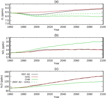
Fig. 6.Time series of the concentrations of O3(a), total reactive nitrogen, NOy(b), and N2O(c)from the REF-B2 (black line), GHG (red line) and CHM (green line) experiments. The concentrations are ensemble averages from 60◦S to 60◦N at 10 hPa
and have been deseasonalized by fitting an 8 term sinusoidal to the monthly averages and smoothed with a Gaussian filter with a width of four years. The first panel also includes the estimate of the ODS effect on ozone derived as (REF-B2–GHG), with the addition of the 1960–1974 average from the REF-B2 experiment (green dashed line).
tion of ozone in the REF-B2 run at 10 hPa returns to 1980 values around 2020, though halogens do not decrease back to 1980 values here until 2050. Ozone in the CHM run, hav-ing constant CO2concentrations, will not be affected by the
CO2-driven cooling in the mid- to upper stratosphere. There
are, however, clearly other effects at work as the concentra-tion of ozone in the CHM run remains well below 1980 val-ues out to 2100, even as halogens return to concentrations found in the mid-1970s. Also shown in panel a is the (REF-B2–GHG) ozone timeseries that, as discussed above, closely follows the concentration of halogens. The ozone timeseries from the CHM experiment steadily diverges from the derived (REF-B2–GHG) timeseries, with small differences apparent as early as the year 2000.
3.4.1 Interactions of nitrogen compounds with GHG-induced changes
The dominant effect explaining the different evolution of ozone in the CHM experiment is the increase in total reac-tive nitrogen (NOy), shown in panel b of Fig. 6, with NOy
concentrations 14% higher over 2080–2099 at 10 hPa than in the REF-B2 or GHG simulations. Note that the differ-ences between the simulations for NOx (NO+NO2) are
al-most identical (13.6%) (not shown). Recalling that all three experiments used identical lower boundary conditions for the chemical CH4and N2O, independent of the radiative effects
nitrogen compounds with GHG-induced changes. The in-teractions of changing GHGs and N2O have been extensively
explored with two-dimensional models (Rosenfield and Dou-glass, 1998; Randeniya et al., 2003; Chipperfield and Feng, 2003). We provide an analysis of the effects here both as an update of the previous studies with a full 3-D CCM, as well as to underline and quantify one other way in which the ef-fects of climate change have been implicitly included in the REF-B2 results.
One aspect of these interactions is illustrated in panel c of Fig. 6, which shows the time series of modelled N2O
at 10 hPa. From 1960–1974 to 2080–2099 the tropospheric concentration of N2O is specified to increase by 24.7% in
the A1B scenario used here. The concentration of N2O at
10 hPa in the CHM simulation closely follows the tropo-spheric change, increasing by 25.0%. However, the con-centration of N2O in the REF-B2 and GHG simulations
creases by 45.8% over the same time. The more rapid in-crease of N2O is a result of the faster B-D circulation in
these two experiments, producing a more rapid transport of air from the troposphere and less time for the photochemical decay of N2O. A lower concentration of reactive nitrogen,
produced as one product of the decay of N2O, is a result.
The rate of decay of N2O may also have changed
be-tween these simulations and may contribute to the observed changes in N2O. The age of air tracer gave an average
age of 4.2 years for all three experiments at 10 hPa for the 1960–1974 period. Given the modelled decay of N2O from
295 ppbv in the troposphere to 95.1 ppbv at 10 hPa, a strato-spheric lifetime of 3.7 years can be derived assuming a first-order decay. By 2080–2099, the average age of air at 10 hPa in the REF-B2 and GHG runs has decreased to 3.2 years and, using the previously derived lifetime, would translate to a N2O concentration at 10 hPa of 155 ppbv taking into
account the increased tropospheric N2O concentration. The
modelled N2O concentration at 10 hPa of 139 ppbv suggests
that the stratospheric lifetime of N2O has, in fact, decreased
(3.3 years) in the REF-B2 and GHG experiments. Therefore, the increase in the concentration of N2O with changes in the
B-D circulation would have been larger based on changes in the average age of air and are, in fact, moderated by a de-crease in the stratospheric lifetime. The dede-crease in lifetime is, to first-order, most likely related to a more rapid vertical transport of N2O to higher levels in the stratosphere where
the photochemical lifetime is shorter.
It is worth noting that with a faster B-D circulation the at-mospheric lifetime of N2O should decrease and, assuming
identical emissions, result in lower tropospheric N2O
con-centrations. The use of a specified concentration as a lower boundary condition (as currently used, to the best of our knowledge, by all CCMs for long-lived trace gases) will ar-tificially constrain the simulation. A similar constraint arises for the halocarbons. The effects on model simulations of re-moving this constraint, by specifying fluxes in place of con-centrations at the lower boundary, is not known.
0 100 200 300 400
N2O (ppbv) 0
5 10 15 20 25
NO
y
(ppbv)
REF−B2 GHG CHM
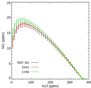
Fig. 7. The relationship between instantaneous concentrations of N2O and reactive nitrogen (NOy) between approximately 150 and
1.0 hPa and 15◦S to 15◦N for the years 2080 and 2083. Data is
taken from one member from each of the three experiments, sam-pled three times a month, and has been binned according to N2O
concentration. Each data point shows the mean concentration of NOyin each bin, with the vertical bars giving the 10th and 90th
per-centiles.
From the earlier 2-D modelling studies it is also well rec-ognized that the cooling of the upper stratosphere by in-creased CO2has important effects on atomic nitrogen and,
by extension, the photochemical loss of NOy. Cooling in the
upper stratosphere will slow the rate of the strongly temper-ature dependent reaction
N+O2→NO+O. (R1)
While the slowing of the rate of this reaction will have no net effect on NOy, it will increase the concentration of atomic N
while having only a very minor effect on the (much larger) concentration of NO. The net effect of the changes will be to increase the rate of loss of NOythrough the reaction
N+NO→N2+O. (R2)
The effects of changes in temperature on reactive nitrogen can be seen in Fig. 7, which presents the instantaneous con-centration of NOyas a function of N2O around the year 2080.
The two experiments with increasing CO2show lower
con-centrations of NOy at the same concentration of N2O than
does the CHM experiment with constant CO2. The
differ-ences are largest at N2O concentrations less than 100 ppbv,
which occur in the mid to upper stratosphere where NOx
−90 −60 −30 0 30 60 90 Latitude 100
10 1
Pressure (hPa)
(a) REF−B2 NOy (ppbv) 1960−1974
1
2 46 8
1012
12
14
(b) REF−B2 Change (ppbv)
−90 −60 −30 0 30 60 90 Latitude 100
10 1
−0.25
−0.25
0.00
0.00
0.00
0.25 0.25
0.50
0.75
(c) CHM Change (ppbv)
−90 −60 −30 0 30 60 90 Latitude 100
10 1
0.25
0.50 0.751.00
1.50
1.50
2.00
2.002.50
Fig. 8. The zonal average distribution of total reactive nitrogen (NOy) in the REF-B2 experiment averaged over 1960–1974(a)
along with the change in the zonal average concentration of NOy
between 1960–1974 and 2080–2099 in the REF-B2(b)and CHM experiments(c). All panels are expressed in ppbv. Note that all three experiments had a very similar distribution of NOyover the
1960–1974 period and that the changes in the GHG simulation are very similar to those shown for the REF-B2 experiment in (b).
with the differences increasing to 25% near the stratopause (not shown). The cooler stratospheric temperatures result-ing from increased CO2give an increase in the concentration
of atomic N and lower concentrations of reactive nitrogen through an increase in the loss rate of NOy.
The net effect of changes in the B-D circulation and the chemistry on the distribution of reactive nitrogen is shown in Fig. 8. Panel a shows the zonal average concentration of NOy
over the period 1960–1974 from the REF-B2 experiment, though the other two experiments show essentially identical distributions over this period. The changes between 1960– 1974 and 2080–2099 for the REF-B2 and CHM experiment are shown in panels b and c, respectively. As noted above, the concentration of N2O entering the stratosphere has increased
by nearly 25%, from 295 to 368 ppbv, between 1960–1974 and 2080–2099, though due to increased tropical upwelling the concentration of NOyin the REF-B2 experiment has
de-creased over much of the stratosphere below 20 hPa. Above 20 hPa, the region where reactive nitrogen chemistry domi-nates the ozone loss reactions, the REF-B2 experiment shows an increase in NOyof between 0.5 and 1.4 ppbv. However,
without the effects of CO2cooling on the upper stratosphere
and the strengthened B-D circulation the increased N2O
pro-duces increases in NOythat are more than twice as large in
the CHM experiment, from 1.5 to 3.0 ppbv, over the same region. These results help explain the finding by Oman et al. (2010) that, through multiple linear regression analysis, changes in NOxhave only a small effect on the future
evo-lution of ozone in simulations with the GEOSCCM model using the same REF-B2 scenario.
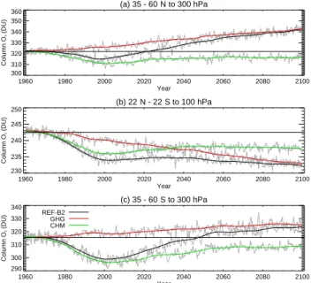
3.5 Column ozone
By comparing the behaviour of the REF-B2 experiment, which contains the effects of increasing ODSs and GHGs, with simulations where one of these forcings was held con-stant, we have explored the ways in which these separate
(a) 35 - 60˚N to 300 hPa
1960 1980 2000 2020 2040 2060 2080 2100
Year 300
310 320 330 340 350 360
Column O
3
(DU)
(b) 22˚N - 22˚S to 100 hPa
1960 1980 2000 2020 2040 2060 2080 2100
Year 230
235 240 245 250
Column O
3
(DU)
(c) 35 - 60˚S to 300 hPa
1960 1980 2000 2020 2040 2060 2080 2100
Year 290
300 310 320 330 340
Column O
3
(DU)
REF-B2 GHG CHM
Fig. 9. Time series of ensemble average column ozone from the REF-B2 (black lines), GHG (red lines) and CHM (green lines) ex-periments over the latitude bands 35–60◦N(a), 22◦N–22◦S (b)
and 35–60◦S(c). To avoid contributions from the troposphere, the
mid-latitude ozone columns are integrated down to 300 hPa and the tropical columns are integrated to 100 hPa. The grey lines give the seasonal anomalies from the deseasonalized data and the coloured lines are the data after smoothing by a Gaussian filter with a width of eight years. The black horizontal line shows the 1960–1974 av-erage from the three experiments.
forcings affect stratospheric ozone over the 21st century. We now look at the net effects on column ozone, the policy-relevant quantity that is directly related to UV radiation lev-els at the surface. Time series of column ozone amounts for the Northern and Southern Hemisphere mid-latitudes and the tropics are presented in Fig. 9. To avoid including changes in the troposphere, for which we have low confidence, column ozone has been calculated by integrating down to 300 hPa for mid-latitude columns and down to 100 hPa for the trop-ics. Column ozone in the GHG experiment shows a con-tinual increase over the length of the experiment in the mid-latitudes, with a considerably greater increase in the Northern than the Southern Hemisphere, and a steady decrease in the tropics. As was seen above, cooling from increasing CO2
ozone over the Northern Hemisphere mid-latitudes than over the Southern Hemisphere mid-latitudes, are consistent with those seen in the suite of CCMVal-2 models (Eyring et al., 2010; SPARC CCMVal, 2010, chapter 9).
As was seen above, the differences between the GHG and REF-B2 experiments are generally well described by the lo-cal concentrations of reactive chlorine and bromine and we thus expect the evolution of column ozone to reflect this. For all latitude bands column ozone in the REF-B2 run follows the longer-term trends of the GHG experiment, with the tran-sient effects of ODSs, peaking around the year 2000 and de-creasing towards 2100, superimposed. Recalling that for the GHG experiment the concentration of ODSs was held con-stant at 1960 values and that ODSs in the REF-B2 run have not completely returned to 1960 values by 2100, we expect column ozone in the REF-B2 run to remain slightly below that in the GHG experiment at 2100. For the period 2080– 2099, differences in column ozone between the REF-B2 and GHG experiments are statistically significant at more than the 99.5% confidence interval for the Southern Hemisphere mid-latitudes and the tropics, while the differences over 35– 60◦
N are only statistically significant at less than the 80% level. Comparing the Northern and Southern Hemisphere mid-latitudes, the variance in the annual column is compara-ble over 2080–2099 and the continued statistical significance of the REF-B2–GHG differences arises primarily from the magnitude of the differences. Earlier, we noted a statisti-cally significant tendency of the (REF-B2–GHG) difference in ozone to lag the trend derived from fitting to EESC in the second half of the 21st century. Referring back to the average residual of the EESC fit shown in Fig. 3, generally negative ozone residuals are found in the lower stratosphere over the 35–60◦
S latitude band, though most of these are not statistically significant. It is unclear, then, to what extent the continued statistically significant effect of ODSs on Southern Hemisphere mid-latitude column ozone over 2080–2099 is a result of the larger perturbation of column ozone by ODSs in the Southern Hemisphere relative to the Northern Hemi-sphere and what portion may be related to the tendency of ozone recovery to lag EESC in parts of the Southern Hemi-sphere.
It has also been shown that reactive nitrogen, driven by in-creasing concentrations of N2O, can have significant effects
on ozone – particularly in the CHM experiment where circu-lation and temperature changes do not moderate the effect of increasing N2O. For all three latitude bands, column ozone
in the CHM experiment initially decreases up to the time of the peak in ODS concentrations around the year 2000. In the absence of perturbations to NOy it could be
reason-ably expected that column ozone would return towards the 1960–1974 baseline as ODSs decrease. In fact, the N2
O-driven increase in NOylimits the recovery of column ozone,
with little additional increase apparent after 2050 and col-umn ozone at 2100 remaining considerably lower than the 1960–1974 average; an evolution much like that found in the
2-D modelling study of Chipperfield and Feng (2003) using a similar scenario. Estimating the contribution of ODSs to ozone changes in the CHM run from the difference (REF-B2–GHG), the increase in NOy(with some additional
con-tribution from H2O) in the CHM run produces a decrease in
column ozone of 4.9 DU in both the Northern and Southern Hemisphere mid-latitudes and a decrease of 3.7 DU in the tropics between 1960–1974 and 2080–2099. The effect of changing NOy on ozone in the REF-B2 and GHG
simula-tions are likely to be considerably smaller than this estimate as the increase in NOywas at most one-half of the increase
of NOyin the CHM experiment.
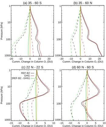
3.6 Vertical distribution of changes in column ozone
The vertical distribution of changes in column ozone is now analyzed to separate the contribution of CO2cooling in the
upper stratosphere from changes in the lower stratosphere. The change in ensemble average ozone relative to the 1960– 1974 average was integrated from 0.1 hPa downward and is shown in Fig. 10 for the periods 1990–2009 and 2080–2099 for the three latitude bands discussed above, in addition to a near-global average covering 60◦
N to 60◦
S. The changes to 1990–2009 (dashed lines) demonstrate the dominant in-fluence of ODSs on ozone, producing decreases in the ozone column above 20 hPa of 5 to 6 DU across the different lati-tude bands as given by the (REF-B2–GHG) difference. The decrease in column above 20 hPa attributed to ODSs is ap-proximately 30 to 35% larger than the decrease in ozone found in the REF-B2 simulation alone, as cooling from CO2
has acted to reverse some of the decrease. For the region of the stratosphere below 20 hPa, large additional decreases in column are found in the Southern Hemisphere mid-latitudes due to the effects of Antarctic ozone depletion, with a much weaker additional decrease in the Northern Hemisphere mid-latitudes. The simulations also demonstrate the effects of changes in the B-D circulation, with tropical ozone (panel c) between 20 and 100 hPa decreasing by 4 DU in the GHG simulation and small increases in the mid-latitude lowermost stratosphere below 100 hPa.
The changes to 2080–2099, given by the solid lines in Fig. 10, show that the effects of ODSs on column ozone in the REF-B2 simulation have generally decreased to less than 1–2 DU, reflecting the decreased concentration of halogens. The changes related to CO2cooling of the upper stratosphere
(a) 35 - 60˚S
-20 -10 0 10 20
Cumm. Change in Column O3 (DU)
1000 100 10 1
Pressure (hPa)
(b) 35 - 60˚N
-20 -10 0 10 20
Cumm. Change in Column O3 (DU)
1000 100 10 1
(c) 22˚N - 22˚S
-15 -10 -5 0 5 10
Cumm. Change in Column O3 (DU)
1000 100 10 1
Pressure (hPa)
REF-B2 GHG (REF-B2 - GHG)
(d) 60˚N - 60˚S
-15 -10 -5 0 5 10
Cumm. Change in Column O3 (DU)
1000 100 10 1
Fig. 10. The vertical integral, from 0.1 hpa downwards, of the change in ozone for the REF-B2 (black) and GHG (red) experi-ments, along with the effects of ODSs derived as the (REF-B2– GHG) difference (green). The changes are relative to the 1960– 1974 average and are shown for 1990–2009 (dashed lines) and 2080–2099 (solid lines) for the latitude bands 35–60◦S(a), 22◦N–
22◦S(b), 35–60◦N(c)and 60◦N–60◦S(d).
the Northern and Southern Hemisphere mid-latitude bands the ozone column shows little net change from 20 hPa down to 90 hPa, while between 90 and 300 hPa ozone increases by a further 10 DU in the Northern Hemisphere with only a 2 to 3 DU increase in the Southern Hemisphere. The large in-crease in ozone in the lowermost stratosphere of the North-ern Hemisphere, and the absence of a similar increase in the Southern Hemisphere, accounts for the differences in the evolution of the column ozone between the hemispheres seen above and is related to the changes in the residual circulation discussed above. Although not displayed here, changes in column ozone in the CHM run show only a small increase of 2 to 3 DU in the lowermost stratosphere, consistent with the more stable B-D circulation in the absence of changes in radiative forcing from long-lived GHGs
The contribution of changes in the tropical lower strato-sphere can also be quantified from panel c of Fig. 10. As for the mid-latitudes, the column amount of ozone above 20 hPa is approximately 7 DU larger in 2080–2099 than in 1960– 1974 in the REF-B2 and GHG experiments. However, the increase in tropical upwelling has reduced ozone between
20 and 100 hPa by approximately 17 DU so that the ozone column at 100 hPa is lower by 10 DU over 2080–2099. As before, though not shown here, we note that the CHM exper-iment shows no similar decreases in column ozone over the tropical lower stratosphere.
We now look at the near-global average of the changes in column ozone shown in panel d of Fig. 10. We have seen above that changes in the residual circulation are pro-jected to have significant effects on ozone in certain loca-tions, though by averaging over 60◦
N to 60◦
S the effects of latitudinal transport of ozone by the residual circulation will be largely removed. Focusing on the results from the GHG experiment, which does not contain the additional effects of ODSs, we see that the ozone column above 20 hPa has in-creased at both 1990–2009 and 2080–2099. Similarly, the ozone between 20 hPa and 200 to 300 hPa has decreased over both time periods. At 2080–2099, the increase above 20 hPa due to CO2cooling is approximately 7 DU and this is very
nearly balanced by decreases through the lower portion of the stratosphere so that column ozone above the tropopause remains little changed. The near-cancellation of changes in the mid to upper stratosphere and the lower stratosphere may be partly a result of “reverse self-healing”, where increases in ozone at higher levels in the atmosphere reduce the produc-tion of ozone at lower levels through increased absorpproduc-tion of solar radiation. Note that in the doubled CO2 experiments
of Fomichev et al. (2007) there was a significant decrease in ozone between about 50 and 20 hPa which could not be accounted for either by circulation changes or by changes in water vapour, so was presumably the result of “reverse self-healing”. Additional possible causes of the decrease seen here include changes in the net amount of ozone due to changes in the residual circulation or chemical effects from increased water vapour. Note that stratospheric water vapour has increased by 1.2 to 1.8 ppmv from 1960–1974 to 2080– 2099 in the REF-B2 and GHG experiments due both to tem-perature changes at the cold point and to increased methane.
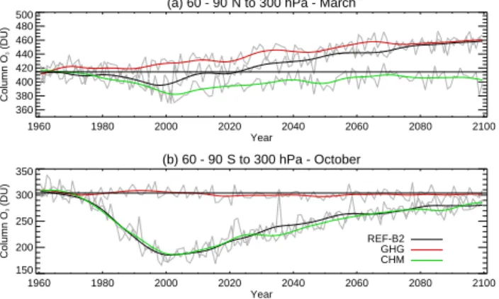
3.7 Column ozone: polar regions
Lastly, we look at polar ozone in the three experiments in Fig. 11, concentrating on the springtime period in each hemi-sphere when ozone depletion is most significant. The March average ozone over 60–90◦