RESEARCH ARTICLE
A Computationally Efficient Filter for
Reducing Shot Noise in Low S/N Data
Mami Okada1, Tomoe Ishikawa1, Yuji Ikegaya1,2*
1Graduate School of Pharmaceutical Sciences, The University of Tokyo, Tokyo, 113–0033, Japan, 2Center for Information and Neural Networks, National Institute of Information and Communications Technology, Suita City, Osaka, 565–0871, Japan
Abstract
Functional multineuron calcium imaging (fMCI) provides a useful experimental platform to simultaneously capture the spatiotemporal patterns of neuronal activity from a large cell populationin situ. However, fMCI often suffers from low signal-to-noise ratios (S/N). The main factor that causes the low S/N is shot noise that arises from photon detectors. Here, we propose a new denoising procedure, termed the Okada filter, which is designed to reduce shot noise under low S/N conditions, such as fMCI. The core idea of the Okada filter is to replace the fluorescence intensity value of a given frame time with the average of two values at the preceding and following frames unless the focused value is the median among these three values. This process is iterated serially throughout a time-series vector. In fMCI data of hippocampal neurons, the Okada filter rapidly reduces background noise and signifi-cantly improves the S/N. The Okada filter is also applicable for reducing shot noise in electrophysiological data and photographs. Finally, the Okada filter can be described using a single continuous differentiable equation based on the logistic function and is thus mathe-matically tractable.
Introduction
Functional multineuron calcium imaging (fMCI) is a promising optical technique that simulta-neously records suprathreshold activity from a large number of neurons [1–3]. An action potential evokes a transient elevation in intracellular calcium ions in the cell body of neurons. By taking advantage of this phenomenon, fMCI infers the times of action potentials from fluc-tuations in the fluorescence intensities in neurons that were loaded with calcium-sensitive fluo-rescent indicators [4]. Typically, an action potential elicits a rapid fluorescence increase that occurs within tens of millisecond, followed by a slow decrease that persists for up to a second [5]. The amplitude of the calcium transients is as small as 2–10% over the baseline intensity when Oregon green 488 BAPTA-1AM (OGB1-AM), the most widely used chemical calcium indicator, is used. Therefore, fMCI is vulnerable to signal-irrelevant noise and often suffers from low signal-to-noise ratios (S/N) [3].
Shot noise is dominant in under low-light intensity conditions during fMCI data acquisi-tion. A major source of shot noise in fMCI is the photodetectors. fMCI mainly uses photomul-tiplier tubes, charge-coupled devices, or complementary metal-oxide-semiconductors to detect
a11111
OPEN ACCESS
Citation:Okada M, Ishikawa T, Ikegaya Y (2016) A Computationally Efficient Filter for Reducing Shot Noise in Low S/N Data. PLoS ONE 11(6): e0157595. doi:10.1371/journal.pone.0157595
Editor:Thomas Abraham, Pennsylvania State Hershey College of Medicine, UNITED STATES
Received:December 13, 2015
Accepted:June 1, 2016
Published:June 15, 2016
Copyright:© 2016 Okada et al. This is an open access article distributed under the terms of the
Creative Commons Attribution License, which permits unrestricted use, distribution, and reproduction in any medium, provided the original author and source are credited.
Data Availability Statement:All relevant data are within the paper.
Funding:This work was supported by Grants-in-Aid for Science Research on Innovative Areas, "Mesoscopic Neurocircuitry" (22115003).
photons. Their signal is inevitably contaminated with internal noise due to the quantal nature of light and the probabilistic nature of photon detection [6]. Thus, the number of photons detected in a given time window could be larger and smaller than the true number, and these stochastic fluctuations cause shot noise.
In fMCI time-series data, shot noise is usually reduced throughpost hocfiltering using a moving window. The filters are classified into two types: linear and nonlinear filters. Most of the linear filters are moving-average low-pass filters with linearly weighted windows, such as rectangular, Gaussian, and Hann windows [7–9]. The basic idea of the linear filters is to replace the value at a focused time with the averaged value over the window. Unfortunately, the linear filters smooth sharply changing values, such as the rising phase of calcium transients, and hin-der the precise detection of the onset times of the calcium transients. Moreover, a single outlier due to shot noise affects nearby values within the window. This undesirable effect is relevant in fMCI data that are acquired at sampling rates as low as tens of hertz.
Nonlinear filters may overcome these problems [10]. A widely used nonlinear filter is the median filter [11]. A median filter replaces the value at a focused time with the median value within a moving window. This procedure tends to preserve the structure of a signal; however, unlike linear filters, a median filter selects the replaced values from a pool of values that already existed in the original data, thereby resulting in less efficient denoising.
In this study, we propose a novel nonlinear filter named the Okada filter, which employs the compromise strategies of linear and median filters. The Okada filter replaces the value at a focused time with the average of two values at both ends of a moving window unless the focused value is the median among values in the window. Therefore, the filtered data contain "more centered" values that did not exist in the original values (as in linear filter) and have a greater likelihood of preserving the structure of the putative signal because any values during a consecutive change are unlikely replaced (as occurs when using a median filter).
Materials and Methods
Animal ethics
Experiments were performed with the approval of the animal experiment ethics committee at the University of Tokyo (approval number: P24-6) and according to the University of Tokyo guidelines for the care and use of laboratory animals.
Functional multineuron calcium imaging
Hippocampal organotypic slices were prepared from Wistar/ST rats (SLC), as described else-where [12]. Rat pups were anaesthetized via hypothermia and isoflurane and then decapitated. The brains were removed and placed in ice-cold oxygenated Gey’s balanced salt solution sup-plemented with 25 mM glucose. The brains were sliced horizontally (300μm thick) using a
vibratome (DTK-1500, Dosaka). Then, entorhinal-hippocampal regions were trimmed using a surgical microknife. The slices were placed on Omnipore membrane filters (JHWP02500, Millipore) and incubated in 5% CO2at 35°C. The culture medium, which was composed of
50% minimal essential medium (Invitrogen), 25% Hanks’balanced salt solution, 25% horse serum (Gibco), and antibiotics, was changed every 3.5 days. Experiments were performed at 11
−19 days in vitro. Slices were transferred to a 35-mm dish that was filled with 2 ml of dye
solu-tion and incubated for 40 min in a humidified incubator at 37°C in 5% CO2with 0.0005%
OGB1-AM (Invitrogen), 0.01% Pluronic F-127 (Invitrogen), and 0.005% Cremophor EL (Sigma-Aldrich) [13]. The slices were then recovered for 30 min in oxygenated artificial cere-brospinal fluid (aCSF) that consisted of (in mM) 127 NaCl, 26 NaHCO3, 3.3 KCl, 1.24
CO2. A slice was mounted in a recording chamber and perfused with aCSF at a rate of 1.5–2.0
ml/min for 15 min. The hippocampal CA3 pyramidal cell layer was imaged at 10 Hz using a Nipkow-disk confocal microscope (CSU-X1, Yokogawa Electric) equipped with a cooled CCD camera (iXonEM+DV897, Andor Technology) and an upright microscope with a water-immersion objective lens (16×, 0.8 numerical aperture, Nikon) [14]. Fluorophores were excited at 488 nm with a laser diode and visualized with a 507-nm long-pass emission filter. The fluo-rescence change was measured as (Ft−F0)/F0, where,Ftis the fluorescence intensity at timet,
andF0is the fluorescence intensity averaged from–10 to 10 s relative tot.
Electrical physiological recording
Recordings were performed in a submerged chamber perfused at 6–8 ml/min with oxygenated aCSF at 35°C. Whole-cell patch-clamp recordings were obtained from hippocampal CA3 pyra-midal cells that were visually identified under an infrared-differential, interference-contrast microscope. For cell-attached recordings, glass pipettes (3–6 MO) were filled with aCSF [15]. For voltage clamp recordings, pipettes were filled with a cesium-based solution that consisted of (in mM) 130 CsMeSO4, 10 CsCl, 10 HEPES, 10 creatine phosphate, 4 Mg-ATP and 0.3 Na2
-GTP [16]. Excitatory postsynaptic currents (EPSCs) were recorded at a clamped voltage of–70 mV. Signals were amplified and digitized at a sampling rate of 2 kHz using a MultiClamp 700B amplifier and a Digidata 1440A digitizer that were controlled by pCLAMP 10.4 software (Molecular Devices).
Okada filter
The Okada filter is given by the following equation:
xt xtþ
xt 1þxtþ1 2xt
2ð1þe aðxt xt 1Þðxt xtþ1ÞÞ ;
wherext–1,xt, andxt+1denote theΔF/Fvalues at framest–1,t, andt+1, respectively. This
equa-tion is based on the logistic funcequa-tion. Therefore, whenαis sufficiently large, it can perform two
processes; (1) if (xt−xt–1)(xt−xt+1)0,xtis substituted withxtitself, and (2) if (xt−xt–1)(xt−xt+1)
>0,xtis substituted with (xt–1+xt+1)/2. This process is repeated subsequently from the second
frame to the penultimate frame, whereas the values from thefirst frame and the last frame are not changed. All routines were written in MATLAB (The MathWorks).
Median filter
Median filter replacesxtwith the median value withinxt–1,xtandxt+1. This process is repeated
subsequently from the second frame to the penultimate frame, whereas the values from the first frame and the last frame are not changed. Unlike the Okada filter, the median filter uses the originalxt–1before substitution asxt–1.
Binomial filter
Binomial filter replacesxtwith a binomial weighted convolution ofxt–1,xtandxt+1(here,xt
0.25xt–1+ 0.5xt+ 0.25xt+1). This replacement is repeated subsequently from the second frame
to the penultimate frame, whereas the values from the first frame and the last frame are not changed. Unlike the Okada filter, the binomial filter uses the originalxt–1before substitution as
xt–1.
Savitzky-Golay filter
Savitzky-Golay filter replacesxtwith the approximate value estimated by fitting a low order
polynomial to a series of {xt–1,xt,xt+1} using the least squared method. This process is repeated
subsequently from the second frame to the penultimate frame, whereas the values from the first frame and the last frame are not changed. Unlike the Okada filter, the Savitzky-Golay filter uses the originalxt–1before substitution asxt–1.
Photograph with shot noise
A portrait of Lenna was downloaded from the Standard Image Data-Base. Shot noise was added with a Poisson distribution as follows:
xi;j ¼
1
poissrndðxi;jÞ
;
wherexi,jrepresents the value of the pixel at rowiand linej. This process was applied to all
pix-els of the photograph.
Peak signal to noise ratio
The peak signal-to-noise ratio (PSNR) is defined using the mean squared error (MSE) as fol-lows:
PSNR¼ 10log p
2
MSE ;
wherepis the maximum luminance value,i.e., 255 for an 8-bit image or 65,025 for a 16-bit image. When the m×n original image (I) was compared to itsfiltered image (K), MSE is given by the following equation:
MSE¼ 1 mn
Xm
i¼1
Xn
j¼1ðIði;jÞ Kði;jÞÞ 2
:
Frequency response
The power spectrum is computed using the Fourier transformation function with a 10-s ham-ming window. The ratio of the power of the filtered trace to that of the original trace at a given frequency is defined as a frequency response.
Statistics
Summarized data are reported as the means ± standard deviations (SDs). For each cell, the log-arithm of the mean amplitude of calcium transients divided by the SD of the fluorescence intensities during baseline periods, except ± 0.5 s relative to the peak of calcium transient, was calculated as the S/N. Wilcoxon signed rank test and pairedt-test were performed to assess the significance of the differences.P<0.05 was considered statistically significant.
Results
Okada filter
The Okada filter is designed to remove outliers in a given time-series vector {xt} (tranges from
following values,xt–1andxt+1, respectively. Ifxtis the median amongxt–1,xt, andxt+1, that is, if
(xt−xt–1)(xt−xt+1)0, thenxtis not changed. Ifxtis not the median, that is, if (xt−xt–1)(xt−xt+1)
>0, thenxtis substituted with the average ofxt–1andxt+1,i.e., (xt–1+xt+1)/2 (Fig 1A). This
pro-cedure is conducted sequentially fromt= 2 to T–1 (Fig 1B). In each step, the value that was updated in the preceding step is used asxt–1. Notably, the substitution process can be expressed
by a single equation using a logistic function (Fig 1C). When the coefficientαis sufficiently large, the equation takes eitherxtor (xt–1+xt+1)/2, depending on the sign of (xt−xt–1)(xt−xt+1).
Specifically, if (xt−xt–1)(xt−xt+1) is negative, the equation substitutesxtwith the same valuext,
otherwise the equation substitutesxtwith (xt–1+xt+1)/2. This conditional substitution is aimed
to filter out a sudden outlier, such as shot noise, in the time-series vector {xt} without affecting
a continuous increase or decrease in {xt} because the latter might reflect signal, such as the
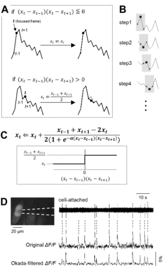
Fig 1. Introduction of the Okada filter. A.Schematic illustration for data processing of the Okada filter. At the focused timet,xtis compared with the preceding and following valuesxt–1andxt+1, respectively. Ifxtis
the median amongxt–1,xt, andxt+1, thenxtis not modified (top). Ifxtis not the median, thenxtis substituted
with the mean ofxt–1andxt+1,i.e., (xt–1+xt+1)/2 (bottom).B.The substitution procedure in A is serially
conducted fromt= 2 to the number of data points−1. In each step, the value updated in the preceding step is
used asxt–1.C.The Okada filter is expressed in a single equation based on the logistic function. The
coefficientαdetermines the steepness in the transition at (xt−xt–1) (xt−xt+1) = 0. Ifαis more than one order
of magnitude higher than the maximal value in {xt}, the transition can be regarded as a digital-like jump.D.
Simultaneous cell-attached unit recording (top) and fMCI from a CA3 pyramidal cell (middle). The fMCI trace was filtered using the Okada filter withα= 100 (bottom). Dashed lines represent the times of action potentials detected in cell-attached trace.
doi:10.1371/journal.pone.0157595.g001
onset of a calcium transient. This conditional process is important to preserve the waveform of signal; note that wildly used filters, such binomial and Savitzky-Golay filters, inevitably smooth the waveforms of sharp signal (e.g., calcium transients in fMCI data) and may lead to erroneous detections of the exact timings of signal onsets (Fig 2). Nonlinear filters, such as the Okada fil-ter and median filfil-ter preserve the true signal onsets (Fig 2).
Filtering fMCI data
We applied the Okada filter to fMCI data. The fluorescence intensities were measured from the cell bodies from CA3 neurons in organotypic hippocampal slice cultures loaded with
OGB1-AM. Because the amplitudes of calcium transients were maximally ~10%, the constant
αwas set to 100. The Okada filter reduced noise from the original calcium trace, embossing the waveforms of spike-evoked calcium transients (Fig 1D). Other examples are shown inFig 3A and 3B, in which the calcium traces of 20 representative neurons were filtered using the Okada filter.
We sought to quantify the denoising power of the Okada filter. We randomly sampled 100 cells from our laboratory data storage and applied the Okada filter. Then, the levels of signal and noise and their ratios (S/N) were compared before and after the filtering (Fig 3C–3E). The mean amplitudes of calcium transients (signal) were significantly reduced in the Okada-filtered traces compared to the original traces (Fig 3C,P= 3.9×10⁻¹⁸,Z= 8.68, Wilcoxon signed rank
test,n= 100 cells). This undesirable signal reduction resulted from substitutions of the peak valuesxtof calcium transients with (xt–1+xt+1)/2. Noise was quantified as the SD of the
fluctu-ations in fluorescence during the baseline periods without calcium transients. Noise was signif-icantly reduced in Okada-filtered trace (Fig 3D,P= 4.5×10⁻¹⁸,Z= 8.67). We calculated the S/
N by dividing the mean amplitudes of calcium transients (signal) by the SD of the baseline fluo-rescence fluctuations (noise). The S/N of the Okada-filtered traces was significantly higher than that of the original traces (Fig 3E,P= 9.6×10⁻¹⁸,Z= 8.58), indicating that the Okada filter
reduces noise to a greater degree than the signal.
Fig 2. The Okada filter does not burr the signal onsets.The original fMCI trace is shown in the top (black), and the black arrowhead indicates the true onset of the calcium transient. In the bottom, each trace after the Okada (orange), median (blue), binomial (red), or Savitzky-Golay (green) filter were superimposed onto the original trace (gray). The colored arrowheads indicate the "detected" onsets of the calcium transient in the filtered traces. Note that both the binomial and Savitzky-Golay filters caused an erroneous shift in the onset time.
Comparison of denoising power
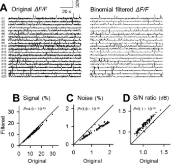
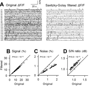
To estimate the merit of the Okada filter, we repeated the same analysis for the median, bino-mial and Savitzky-Golay filters (Figs4A,5Aand6A;n= 100 cells). To facilitate comparisons, the identical datasets were filtered. All these filters also reduced the signal and noise (Fig 4B,
P= 1.2×10⁻¹⁷,Z= 8.55;Fig 4C,P= 3.9×10⁻¹⁸,Z= 8.68;Fig 5B,P= 4.0×10⁻¹⁸,Z= 8.68;Fig 5C, P= 3.9×10⁻¹⁸,Z= 8.68;Fig 6B,P= 5.0×10⁻¹⁸,Z= 8.65;Fig 6C,P= 3.9×10⁻¹⁸,Z= 8.68) and
increased the S/N (Fig 4D,P= 3.9×10⁻¹⁸,Z= 8.68;Fig 5D,P= 5.1×10⁻¹⁸,Z= 8.65;Fig 6D, P= 5.1×10⁻¹⁸,Z= 8.65).
Fig 3. Application of the Okada filter to fMCI data. A.In a confocal image of the CA3 region of cultured hippocampal slices loaded with OGB1-AM (top), the cell bodies of neurons were identified (bottom).B.Left 20 traces are raw fluctuations in the OGB1 fluorescence intensities in the cell bodies numbered inAand were Okada-filtered (right).C.Comparison of the mean signal, the mean amplitude of calcium transients that occurred in individual cells, before (abscissa) and after Okada filtering (ordinary). Each dot indicates a single cell.D.The same asC, but for the background noise level, the SDs in fluorescence intensities during the baseline period in the absence of calcium transients.E.The same asC, but for the S/N ratio, the mean signal divided by the background noise level.Pwas determined using Wilcoxon signed rank test for 100 cells.
doi:10.1371/journal.pone.0157595.g003
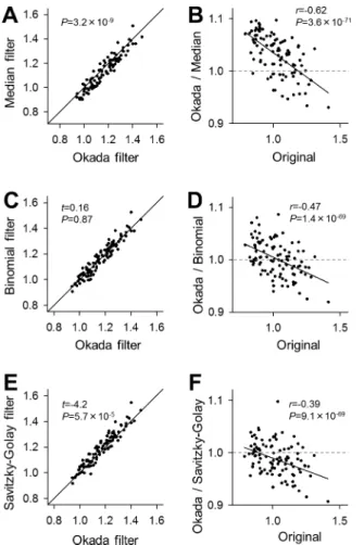
We compared the S/N of the Okada-filtered and median filtered traces (Fig 7A). The S/N varied among datasets; however, as a whole, the Okada filter produced significantly higher S/N than did the median filter (Fig 7A,P= 3.2×10⁻⁹,Z= 5.92). This difference appeared to be due Fig 4. Application of the median filter to fMCI data. A.Left 20 traces are raw fluctuations in the OGB1 fluorescence intensities in the cell bodies numbered inFig 3Aand were median-filtered (right).B-D.
Comparison of the signal (B), the background noise level (B) and its ratio (D) before and after median filtering. Each dot indicates a single cell.Pwas determined using Wilcoxon signed rank test for the same 100 cells as those used inFig 3C–3E.
doi:10.1371/journal.pone.0157595.g004
Fig 5. Application of the binomial filter to fMCI data. A. Left 20 traces are raw fluctuations in the OGB1 fluorescence intensities in the cell bodies numbered inFig 3Aand were binomial-filtered (right).B-D. Comparison of the signal (B), the background noise level (C) and its ratio (D) before and after binomial filtering. Each dot indicates a single cell.Pwas determined using Wilcoxon signed rank test for the same 100 cells as those used inFig 3C–3E.
to the greater ability of the Okada filter to remove baseline noise. Therefore, to examine whether the noise level affected the performance of these filters, we plotted the ratios of the S/N of Okada-filtered traces to those of median-filtered traces against the S/N of the original traces. These parameters exhibited a negative correlation (Fig 7B, Pearson’sr=−0.62,P= 3.6×10−71,
t98= 50), and the regression line crossedy= 1 at the S/N of 1.19 dB. Thus, the Okada filter
removed noise more efficiently from the lower S/N data. We also compared the S/N of the Okada-filtered traces with the binomial-filtered and Savitzky-Golay-filtered traces in the same manner. The Okada filter improved the S/N to a degree that was comparable to the binomial filter (Fig 7C,t= 0.16,P= 0.87, pairedt-test) but that was lower than the Savitzky-Golay filter (Fig 7E,t= 4.2,P= 5.7×10⁻⁵). The high performances of binomial and Savitzky-Golay filters
were presumably because these filters preserve the signal amplitude more than the Okada filter. However, like theFig 7Bplot, theFig 7D and 7Fplots also exhibited a negative correlation (Fig 7D, Pearson’sr=−0.47,P= 1.4×10−69,t98= 48;Fig 7F, Pearson’sr=−0.39,P= 9.1×10−69,
t98= 47). These results confirm that the Okada filter worked relatively efficiently in the lower
S/N data.
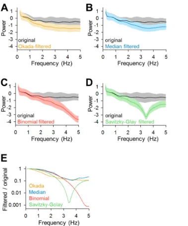
We computed the power spectra of the original traces and the traces that were filtered by the Okada, median, binomial and Savitzky-Golay filters (Fig 8A–8D,n= 100). Then we plotted the frequency responses, the ratios of the powers of the filtered traces to that of the original traces (Fig 8E). The Okada and median filters broadly reduced the power with a low-pass trend, whereas the binominal and Savitzky-Golay filters reduced the power in a more fre-quency-specific manner.
Comparison of computational speed
We next measured the computing speed of the Okada filter. We used a commercially available laptop computer equipped with Intel1Core™i5-3337U Processor (64 bit, 1.80 GHz) and 8.0
Fig 6. Application of the Savitzky-Golay filter to fMCI data. A. Left 20 traces are raw fluctuations in the OGB1 fluorescence intensities in the cell bodies numbered inFig 3Aand were Savitzky-Golay-filtered (right). B-D. Comparison of the signal (B), the background noise level (C) and its ratio (D) before and after Savitzky-Golay filtering. Each dot indicates a single cell.Pwas determined using Wilcoxon signed rank test for the same 100 cells as those used inFig 3C–3E.
doi:10.1371/journal.pone.0157595.g006
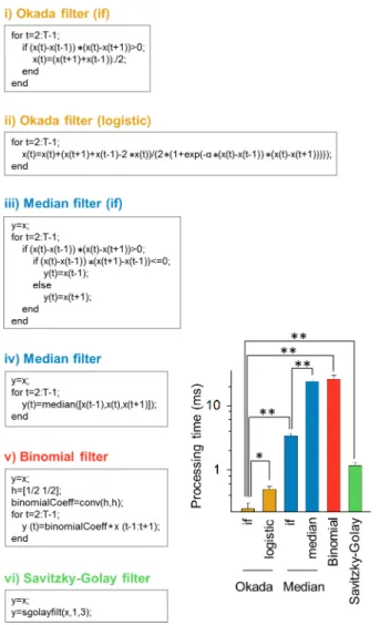
GB RAM. Using the MATLAB code based the 'if/else' statement inFig 9i), we filtered 100 cal-cium traces used above. These data were taken at 10 frames per second for 300 s and thus con-tained 3,000 data points. The computation time spent to filter a single trace was, on average, 247 ± 58μs (mean ± SD of 100 cells). The Okada filter can be expressed using the logistic
func-tion (Fig 9ii). That the commands executed inFig 9i) and9ii) are theoretically identical, but the computation time ofFig 9ii) was 499 ± 51μs and was twice longer than that ofFig 9i)
(P= 2.1×10⁻¹⁷,Z= 8.49, Wilcoxon signed rank test,n= 100). This difference is probably
because the exponential function demanded a higher computational cost. We also measured the computational speed of the median filter.Fig 9iii) uses the 'if' statement to examine whether
xtis the median. Its computational time was 3.76 ± 0.85 ms and was approximately 14 times
longer than that ofFig 9i) (P= 3.9×10⁻¹⁸,Z= 8.68). If we used a MATLAB function 'median',
the computational time increased further to 23.7 ± 1.6 ms. Moreover, we examined the compu-tational speed of the binomial and Savitzky-Golay filters using the MATLAB codes described
Fig 7. Comparison of S/N improved by the Okada and the median, binomial, and Savitzky-Golay filters. A.The S/N is compared between Okada-filtered (abscissa) and median-filtered traces (ordinary). Each dot represents a single cell. Wilcoxon signed rank test.n= 100 cells.B.The ratios of the S/N in the Okada-filtered traces to those in median-filtered traces are plotted against the S/N in the original raw traces. Pearson’s correlation coefficientrwas negative, and the regression line crossedy= 1 at the original S/N of 1.19.C. Same asA, but compared to the binomial-filtered traces.D. Same asB, but for binomial-filtered traces. Pearson’s correlation coefficientrwas negative, and the regression line crossedy= 1 at the original S/N of 1.04.E. Same asA, but compared to Savitzky-Golay-filtered traces.F. Same asB, but for Savitzky-Golay-filtered traces. Pearson’s correlation coefficientrwas negative, and the regression line crossedy= 1 at the original S/N of 0.90.
inFig 9v) and vi). Their computational times were 26.0 ± 3.4 ms and 1.17 ± 0.15 ms, respec-tively, and were both significantly longer than the Okada filter (bothP= 3.9×10⁻¹⁸,Z= 8.68).
Thus, the Okada filter is superior to the other filters in terms of computational speed. The rapid computation of the Okada filter is mainly due to the fact that it can skips the substituting process when the focused valuextis the median; note that the linear filter has to update all
val-ues in the vector.
Effect of the window length of Okada filter on denoising performance
In most of the denoising filters, the window length is modifiable. Therefore, we compared the performance of the Okada filters with different window lengths. To preserve the amplitude of signal, we changed the substitutional procedure of the Okada filter. Specifically, the focused valuextis not changed if it is the median among the values within the window, whereas ifxtis
not the median,xtis substituted with the average of three points around the median,i.e., the
median and two immediately higher and lower values (two nearest neighbor values) of the median within the window. We applied the Okada filters with different window lengths, three, five and seven frames, to fMCI data. In all cases, the filters reduced the noise of traces (Fig 10, left) and improved the S/N (Fig 10, middle, window = 3,P= 9.6×10⁻¹⁸,Z= 8.58, window = 5, P= 6.3×10⁻¹⁷,Z= 8.36, window = 7,P= 4.7×10⁻¹⁶,Z= 8.12, Wilcoxon signed rank test, n= 100). Compared to the window of three frames (the original Okada filter), the filter with
Fig 8. Comparisons of the frequency responses of the Okada, median, binomial, and Savitzky-Golay filters. A. The mean±SD power spectra of the 100 cells data same as used inFig 3are shown in black, where those of Okada-filtered traces are shown in color.B-D. Same asA, but for the median (B, blue), binomial (C, red) and Savitzky-Golay (D, green) filtered traces.E. The mean frequency response of each filter is shown relative to the mean powers of the original traces.
doi:10.1371/journal.pone.0157595.g008
longer window improved the S/N more effectively (Fig 10, right, window = 5,P= 1.8×10⁻¹⁰, Z= 6.38, window = 7,P= 1.3×10⁻⁸,Z= 5.68). Thus, the Okada filter with longer window
improved the S/N of fMCI data more efficiently.
Modified Okada filters
The mean filter can be modified to the binomial and Gaussian filters using appropriate weight-ing factors. Likewise, the Okada filter can also be modified by changweight-ing the coefficientβin the equation inFig 11A; higherβconditions preservextmore heavily in the replaced value. That is,
the modified Okada filter is expected to work more similarly to a binomial filter when the value replacement occurs. We thus tested the performance of the modified Okada filter with different values ofβ>2 (Fig 11B, left). Under allβconditions tested, the modified filter improved the S/ N of fMCI data (Fig 11B, middle,β= 2,P= 1.3×10⁻¹⁷,Z= 8.54;β= 3,P= 8.8×10⁻¹⁸,Z= 8.59;
β= 4,P= 8.3×10⁻¹⁸,Z= 8.60;β= 5,P= 9.3×10⁻¹⁸,Z= 8.58;β= 6,P= 6.1×10⁻¹⁸,Z= 8.63;β=
7,P= 5.3×10⁻¹⁸,Z= 8.63;β= 8,P= 6.1×10⁻¹⁸,Z= 8.63;β= 9,P= 6.1×10⁻¹⁸,Z= 8.63;β= 10, Fig 9. Comparison of computational speed of the Okada and median, binomial, and Savitzky-Golay filters.The statement of each left box is the MATLAB command lines executed in the corresponding filter. Note that the statements i) and ii) and the statements iii) and iv) are theoretically identical but are differently described. The bar graph indicates the mean±SD times spend in computing in these MATLAB codes.
*P= 2.1×10⁻¹⁷,**P= 3.9×10⁻¹⁸; Wilcoxon signed rank test.n= 100 cells.
P= 6.1×10⁻¹⁸,Z= 8.63, Wilcoxon signed rank test,n= 100). Compared to the original Okada
fil-ter (β= 2), the effect of the modified Okada filters with higherβvalues were less sufficient to the low S/N data (Fig 11B, right,β= 3, Pearson’sr= 0.41,P= 2.4×10−76,t
98= 56;β= 4,r= 0.22,
P= 1.8×10−65,t
98= 43;β= 5,r= 0.50,P= 5.5×10−57,t98= 35;β= 6,r= 0.51,P= 2.0×10−52,t98=
31;β= 7,r= 0.50,P= 1.6×10−47,t
98= 27;β= 8,r= 0.52,P= 4.0×10−46,t98= 26;β= 9,r= 0.52,
P= 3.6×10−44,t
98= 25;β= 10,r= 0.52,P= 1.2×10−42,t98= 24). As a result, the S/N of the filtered
traces were the highest atβ= 2 (the Okada filter) and were decreased with largerβ(Fig 11C).
Further applications of the Okada filter
Although we originally developed the Okada filter to denoise vector sequences with low S/N and with low temporal resolution, such as fMCI data, we finally tried to apply it to other forms of data.
We first filtered electrophysiological data acquired at a high temporal resolution (Fig 12). Excitatory postsynaptic currents were recorded at 2 kHz from CA3 pyramidal cells in a hippo-campal slice culture. The Okada filter and the median filter both reduced the baseline noise; however, there was still noise in the filtered traces. We thus repetitively applied the filters and found a critical difference in the denoising performance between the Okada filter and the median filter, particularly in later stages of the iterations. Noise was gradually reduced when the Okada filter was repeated, but the median filter did not show this effect. The Okada filter fundamentally substitutesxtwith a new value that is different fromxt–1,xt, orxt+1. Conversely,
the median filter necessarily selects a substituted value from eitherxt–1,xt, orxt+1, and thus, the
effect of iterative filtering is limited.
Fig 10. Application of the Okada filter with different window lengths to fMCI data.The original fMCI trace (top) was filtered by the Okada filters with window lengths of three, five and seven frames (left). The same fMCI data asFig 3were filtered. The S/Ns in the filtered traces were compared to the original S/Ns (middle), and the effect of the Okada filter with the windows of five and seven frames was compared to that with three frames (right).
doi:10.1371/journal.pone.0157595.g010
We also investigated the effect of the Okada filter on photo images with shot noise. The Okada filter compares values of three neighboring points in a one-dimensional vector {xt}, and
this idea cannot be applied to two-dimensional (2D) matrix {xi,j}. Therefore, we made a small
modification. The 2D-modified Okada filter substitutesxi,jwith the average of the vertically
and horizontally scanned Okada-filtered values. This process is expressed by the following
Fig 11. Application of the modified Okada filters to fMCI data. A. The modified Okada filter is expressed in the equation similar to that shown inFig 1C, but the coefficientβin the denominator can take a value different from 2.B. The original fMCI trace (top) was filtered by the Okada filter (β= 2) and the modified Okada filters (β= 3–10). The same fMCI data asFig 3were filtered. The S/Ns in the filtered traces were compared to the original S/Ns (middle), and the effect of the modified Okada filter was compared to the Okada filter (right).C. The mean±SEM S/Ns of the 100 filtered traces are
plotted as a function ofβ.
equation:
xi;j xi;jþ
xi 1;jþxiþ1;j 2xi;j
2f1þe aðxi;j xi 1;jÞðxi;j xiþ1;jÞgþ
xi;j 1þxi;jþ1 2xi;j
2f1þe aðxi;j xi;j 1Þðxi;j xi;jþ1Þg
=2:
One representative video frame of fMCI is shown inFig 13A, which contains shot noise because it was taken under low-light intensity conditions. Because the data were presented in the form of a 16-bit digital image,αwas set to 106. When the Okada filter and the median filter were applied to this image, shot noise was reduced and the contours of individual neurons could be more easily identified (Fig 13A). We also filtered a natural photograph (portrait) in which the shot noise was artificially added. The Okada filter and the median filter both success-fully smoothed out shot noise (Fig 13C). In both images, we calculated the PSNR to evaluate the denoising effect of the Okada and median filters. The PSNR of the fMCI image inFig 13A
and the photograph inFig 13Cwere both higher than the original image (Fig 13B, original ver-susOkada, originalversusmedian,P= 1.8×10⁻⁵,Z= 4.29, Wilcoxon signed rank test,F
23,23=
2.13, 2.20,F-test of equality of variances,n= 24 subregions;Fig 13D,P= 1.03×10⁻²⁰and
2.44×10⁻²¹,t
15= 32.5 and 34.6, pairedt-test,F15,15= 1.43 and 1.08, respectively,n= 16
com-partments.). In the fMCI image, the Okada filter was slightly inferior to the medial filter in terms of the PSNR evaluation (P= 4.5×10⁻¹²,t
23= 13.0, pairedt-test,F23,23= 1.03).
Discussion
In this study, we devised an Okada filter, a novel nonlinear filter that is optimized to data with low S/N and with low sampling rates. Indeed, the Okada filter reduces noise in fMCI data and
Fig 12. Application of the Okada and median filters to electrophysiological data.A raw EPSC trace acquired using whole-cell voltage-clamped recording at 2 kHz (top) was repeatedly filtered up to five times using the Okada (left) and median filters (right). Note that the background noise is reduced even more when the Okada filtering is repeated more.
doi:10.1371/journal.pone.0157595.g012
improves their S/N. We compared the performance of the Okada filter to that of the median fil-ter, binomial filter and Savitzky-Golay filter. The Okada filter surpassed the median filter in denoising and computational speed. Moreover, the Okada filter showed a higher computa-tional speed than the binomial and Savitzky-Golay filters. Therefore, the Okada filter is more suitable for practical use. The frequency response analysis revealed that the Okada filter broadly reduces high frequency components, suggesting that the Okada filter works more effectively for white noise-like background fluctuations, such as thermal noise. In addition, the modified Okada filter also improved the S/N of the fMCI data. One may be able to adjust the parameterβto a given purpose.
The S/N in fMCI has been improved by development of more sensitive calcium indicators and more optimized optical systems, such as objective lens and photodetectors [17]; however, their shot noise is stochastically emitted during the process of photon conversion and can
Fig 13. Application of the Okada and median filters to photographs. A.A single frame of fMCI (top) was Okada-filtered (middle) and median-filtered (bottom).B.The PSNR was compared between the original image and the Okada-filtered or median-filtered images shown inA.*P= 1.8×10⁻⁵,Z= 4.29, Wilcoxon signed rank test (F
23,23= 2.13, 2.20,F-test of equality
of variances);**P= 4.5×10⁻¹²,t
23= 13.0, pairedt-test (F23,23= 1.03,F-test of equality of variances), mean±SEM of 24
subregions.C. The same asA, but for a photograph to which shot noise was artificially added.D. The PSNR was compared between the original image and the Okada- or median-filtered images shown inC.*P= 1.03×10⁻²⁰and 2.44×10⁻²¹, respectively,t15= 32.5, 34.6, pairedt-test (F15,15= 1.43, 1.08,F-test of equality of variances), mean±SEM of 16
compartments.
come from cosmic rays. Thus, online removal of the shot noise during image acquisition is technically difficult. Therefore, fMCI data are usually denoised using offline filters that are employed in image processing and sound processing [10,18,19]. Each filter has advantages and disadvantages. Linear filters are usually effective in reducing high-frequency noise, including shot noise; however, because of their nature, they often blur the edges of the signal and thereby deform the shapes of the signal. Conversely, nonlinear filters have less influence on the edges, but their denoising powers may be insufficient. In this way, the Okada filter reduces noise by averaging values within a window, such as the linear filter, and leaves the putative signal, such as the median filter, thereby benefitting from the advantages of both types of filters. Further-more, we found that the Okada filter with longer windows improved the S/N of fMCI traces more efficiently. Because the amplitudes of signal tended to be more severely reduced when using longer windows (relatively to the frame rates), the Okada filters with long windows may be suitable for fMCI data recorded at higher temporal resolution. In the Okada filter, the parameterβis modifiable to optimize its denoising power depending on the S/N of the original data. Some of the recently developed calcium indicators are sensitive enough to exhibit the sig-nal amplitude larger than 50% over the baseline intensity. In such cases with excellent S/N, higherβvalues might be suitable.
Another disadvantage of nonlinear filters is, in general, the high cost for von Neumann computation; however, the Okada filter is a nonlinear filter that exhibits more rapid computa-tion than the median filter. Its computacomputa-tional speed is almost a match for that of simple linear filters. This efficient computation may be applicable to an immediate filter that works online during data sampling. Moreover, we packed the data processing of the Okada filter into a single mathematical formula, while the median filter cannot be formulated in a single algebraic equa-tion. The equation of Okada filter is a continuous, integrable, and differentiable funcequa-tion. Thus, it is not only arithmetically tractable but may be also applicable to development of elec-tric circuit-based denoising devices.
Acknowledgments
We thank Mr. Nariaki Uemura for his initial trials of the Okada filter and Mr. Tetsuya Sakagu-chi for optimizing MATLAB codes.
Author Contributions
Conceived and designed the experiments: MO YI. Performed the experiments: TI. Analyzed the data: MO. Contributed reagents/materials/analysis tools: YI. Wrote the paper: MO YI.
References
1. Takahashi N, Sasaki T, Usami A, Matsuki N, Ikegaya Y (2007) Watching neuronal circuit dynamics through functional multineuron calcium imaging (fMCI). Neurosci Res 58: 219–225. PMID:17418439 2. Namiki S, Ikegaya Y (2009) Current application and technology of functional multineuron calcium
imag-ing. Biol Pharm Bull 32: 1–9. PMID:19122272
3. Takahashi N, Oba S, Yukinawa N, Ujita S, Mizunuma M, Matsuki N, et al. (2011) High-speed multi-neuron calcium imaging using Nipkow-type confocal microscopy. Curr Protoc Neurosci 2: 14. doi:10. 1002/0471142301.ns0214s57PMID:21971847
4. Smetters D, Majewska A, Yuste R (1999) Detecting action potentials in neuronal populations with cal-cium imaging. Methods 18: 215–221. PMID:10356353
5. Sasaki T, Takahashi N, Matsuki N, Ikegaya Y (2008) Fast and accurate detection of action potentials from somatic calcium fluctuations. J Neurophysiol 100: 1668–1676. doi:10.1152/jn.00084.2008PMID: 18596182
6. Sjulson L, Miesenbock G (2007) Optical recording of action potentials and other discrete physiological events: a perspective from signal detection theory. Physiology (Bethesda) 22: 47–55.
7. Savitzky A, Golay MJE (1964) Smoothing and differentiation of data by simplified least squares proce-dures. Anal Chem 36: 1627–1639.
8. Little MA, Jones NS (2013) Signal processing for molecular and cellular biological physics: an emerging field. Philos Trans A Math Phys Eng Sci 371: 20110546. doi:10.1098/rsta.2011.0546PMID:23277603 9. Ikegaya Y, Aaron G, Cossart R, Aronov D, Lampl I, Ferster D, et al. (2004) Synfire chains and cortical
songs: temporal modules of cortical activity. Science 304: 559–564. PMID:15105494
10. Yaksi E, Friedrich RW (2006) Reconstruction of firing rate changes across neuronal populations by temporally deconvolved Ca2+imaging. Nat Methods 3: 377
–383. PMID:16628208
11. Arias-Castro E, Donoho DL (2009) Does median filtering truly preserve edges better than linear filter-ing? Annal Stat 37: 1172–1206.
12. Koyama R, Muramatsu R, Sasaki T, Kimura R, Ueyama C, Tamura M, et al. (2007) A low-cost method for brain slice cultures. J Pharmacol Sci 104: 191–194. PMID:17558179
13. Ishikawa T, Okamoto K, Ikegaya Y (2015) Homeostatic hippocampal activity against reduced glutama-tergic neurotransmission. Int J Pharmacol 11: 318–326.
14. Mizunuma M, Norimoto H, Tao K, Egawa T, Hanaoka K, Sakaguchi T, et al. (2014) Unbalanced excit-ability underlies offline reactivation of behaviorally activated neurons. Nat Neurosci 17: 503–505. doi: 10.1038/nn.3674PMID:24633127
15. Sasaki T, Matsuki N, Ikegaya Y (2011) Action-potential modulation during axonal conduction. Science 331: 599–601. doi:10.1126/science.1197598PMID:21292979
16. Takahashi N, Kitamura K, Matsuo N, Mayford M, Kano M, Matsuki N, et al. (2012) Locally synchronized synaptic inputs. Science 335: 353–356. doi:10.1126/science.1210362PMID:22267814
17. Grienberger C, Konnerth A (2012) Imaging calcium in neurons. Neuron 73: 862–885. doi:10.1016/j. neuron.2012.02.011PMID:22405199
18. Fiore L, Corsini G, Geppetti L (1996) Application of non-linear filters based on the median filter to exper-imental and simulated multiunit neural recordings. J Neurosci Methods 70: 177–184. PMID:9007757 19. Szymanska AF, Kobayashi C, Norimoto H, Ishikawa T, Ikegaya Y, Nenadic Z Accurate detection of low