www.clim-past.net/12/1739/2016/ doi:10.5194/cp-12-1739-2016
© Author(s) 2016. CC Attribution 3.0 License.
Bering Sea surface water conditions during Marine Isotope
Stages 12 to 10 at Navarin Canyon (IODP Site U1345)
Beth E. Caissie1, Julie Brigham-Grette2, Mea S. Cook3, and Elena Colmenero-Hidalgo4 1Iowa State University, Ames, Iowa, USA
2University of Massachusetts Amherst, Amherst, Massachusetts, USA 3Williams College, Williamstown, Massachusetts, USA
4Universidad de León, León, Spain
Correspondence to:Beth E. Caissie (bethc@iastate.edu)
Received: 8 December 2015 – Published in Clim. Past Discuss.: 19 January 2016 Revised: 4 July 2016 – Accepted: 31 July 2016 – Published: 1 September 2016
Abstract. Records of past warm periods are essential for understanding interglacial climate system dynamics. Marine Isotope Stage 11 occurred from 425 to 394 ka, when global ice volume was the lowest, sea level was the highest, and terrestrial temperatures were the warmest of the last 500 kyr. Because of its extreme character, this interval has been con-sidered an analog for the next century of climate change. The Bering Sea is ideally situated to record how opening or clos-ing of the Pacific–Arctic Ocean gateway (Berclos-ing Strait) im-pacted primary productivity, sea ice, and sediment transport in the past; however, little is known about this region prior to 125 ka. IODP Expedition 323 to the Bering Sea offered the unparalleled opportunity to look in detail at time peri-ods older than had been previously retrieved using gravity and piston cores. Here we present a multi-proxy record for Marine Isotope Stages 12 to 10 from Site U1345, located near the continental shelf-slope break. MIS 11 is bracketed by highly productive laminated intervals that may have been triggered by flooding of the Beringian shelf. Although sea ice is reduced during the early MIS 11 laminations, it remains present at the site throughout both glacials and MIS 11. High summer insolation is associated with higher produc-tivity but colder sea surface temperatures, which implies that productivity was likely driven by increased upwelling. Mul-tiple examples of Pacific–Atlantic teleconnections are pre-sented including laminations deposited at the end of MIS 11 in synchrony with millennial-scale expansions in sea ice in the Bering Sea and stadial events seen in the North At-lantic. When global eustatic sea level was at its peak, a se-ries of anomalous conditions are seen at U1345. We
exam-ine whether this is evidence for a reversal of Bering Strait throughflow, an advance of Beringian tidewater glaciers, or a turbidite.
1 Introduction
Predictions and modeling of future climate change require a detailed understanding of how the climate system works. Reconstructions of previous warm intervals shed light on in-terhemispheric teleconnections. The most recent interglacial period with orbital conditions similar to today was approxi-mately 400 ka, during the extremely long interglacial known as Marine Isotope Stage (MIS) 11. CO2 concentration av-eraged approximately 275 ppm, which is similar to pre-industrial levels (EPICA Community Members, 2004). The transition from MIS 12 into MIS 11 has been compared to the last deglaciation (Dickson et al., 2009), and extreme warmth during MIS 11 has been considered an analog for future warmth (Droxler et al., 2003; Loutre and Berger, 2003), al-though the natural course of interglacial warmth today has been disrupted by anthropogenic forcing (IPCC, 2013).
(De-ODP 884
GA AS
BS Nome
Kotzebue
Bering Sea
Chukchi Sea
SLI
P
B Lake
El’gygytgyn
U1345
Arci
c coastal pla
in
N
ANS BSC
Alaska
n Strea
m
KC
Eas t Siberian Sea
Beaufort Sea
U1343
U1340 U1341
140° W 160° W
180° 160° E
70° N
60° N
50° N
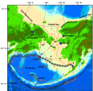
Figure 1.Map of Beringia with locations of cores mentioned in the text (U1345 (red dot), and U1340, U1341, U1343, and ODP Site 884 (grey dots)). Locations of place names from the text are labeled: Aleutian North Slope Current (ANS), Anadyr Strait (AS), Bristol Bay (B), Bering Strait (BS), Bering Slope Current (BSC), Gulf of Anadyr (GA), Kamchatka Current (KC), Navarin Canyon (N), Pribilof Islands (P), and St. Lawrence Island (SLI). The white-and-black dashed line is the maximum extent of sea ice (median over the period 1979–2013) (Cavalieri et al., 1996). Currents are in orange and are modified from Stabeno (1999). Base map is modified from Manley (2002).
Boer and Nof, 2004; Hu et al., 2010); however, there have been no tests of these modeling studies using proxy data older than 30 ka. Furthermore, the location of the Bering Sea marginal sea ice zone advanced and retreated hundreds of kilometers during the past three glacial–interglacial cycles (Caissie et al., 2010; Katsuki and Takahashi, 2005; Sancetta and Robinson, 1983); however, sea surface and intermediate water variability before MIS 5 is unknown.
This investigation of terrestrial–marine coupling at the shelf-slope break from MIS 12 to 10 is the first study of this interval in the subarctic Pacific (Fig. 1). We use a multi-proxy approach to examine orbital- and millennial-scale changes in productivity and sea ice extent. We demonstrate that insola-tion plays a major role in these changes but that sea ice also shows rapid, millennial-scale variability. Finally, we test the hypotheses that (1), in Beringia, tidewater glaciers advanced while sea level was high and (2) Bering Strait throughflow reversed shortly after the MIS 12 glacial termination (Termi-nation V). We find inconclusive evidence of a glacial advance but no evidence of Bering Strait reversal.
2 Background
2.1 Global and Beringian sea level during MIS 11 The maximum height of sea level during MIS 11 is an open question with estimates ranging from 6 to 13 m above present sea level (a.p.s.l.) (Dutton et al., 2015) to 0 m a.p.s.l. (Rohling et al., 2010; Rohling et al., 2014). The discrepancy may stem from large differences between global eustatic (Bowen, 2010) or ice-volume averages (McManus et al., 2003) and re-gional geomorphological or micropaleontological evidence (van Hengstum et al., 2009). Regional isostatic adjustment due to glacial loading and unloading is now known to be significant, and regional highstands may record higher than expected sea levels if glacial isostasy and dynamic topogra-phy have not been accounted for, even in places that were never glaciated (PAGES Past Interglacials Working Group, 2016; Raymo and Mitrovica, 2012; Raymo et al., 2011). For example, Raymo and Mitrovica (2012) suggest eustatic sea level during MIS 11 was 6–13 m a.p.s.l. globally and near 5 m a.p.s.l. locally in Beringia, yet MIS 11 shorelines are at+22 m today in northwestern Alaska (Kaufman and Brigham-Grette, 1993) due to these complex geophysics.
Regardless of the ultimate height of sea level, the transition from MIS 12 to MIS 11 records the greatest change in sea level of the last 500 ka (Rohling et al., 2014); sea level rose from perhaps−140 m to its present level or higher (Bowen, 2010; Dutton et al., 2015). Sea level history during MIS 11 may have been complex (Kindler and Hearty, 2000), but most records agree that sea level during this exceptionally long interglacial (30 kyr) was highest from 410 to 401 ka, coinci-dent with a second peak in June insolation at 65◦N. This long
highstand most likely requires partial or complete collapse of the Greenland Ice Sheet (up to 6 m) (de Vernal and Hillaire-Marcel, 2008; Reyes et al., 2014) and/or the West Antarctic Ice Sheet (Scherer et al., 1998), but not the East Antarctic Ice Sheet (PAGES Past Interglacials Working Group, 2016; Dutton et al., 2015; Raymo and Mitrovica, 2012). It has fre-quently been hypothesized that the West Antarctic Ice Sheet collapsed during MIS 11, and modeling studies confirm this (Pollard and DeConto, 2009); however, unconformities in the record prevent confirmation of a collapse (McKay et al., 2012). Yet, Teitler (2015) show that ice-rafted debris (IRD) during MIS 11 dropped as low as it was during MIS 31, when it is clear that the West Antarctic Ice Sheet had collapsed (Naish et al., 2009). With uncertainties, East Antarctic ice was stable; however, small changes in either sector of the Antarctic Ice Sheet may have contributed up to 5 m of sea level rise (PAGES Past Interglacials Working Group, 2016; EPICA Community Members, 2004).
160° W 140° W 180°
160° E 70° N
60° N
50° N (a)
160° W 140° W 180°
160° E
(b)
Glacial ice
Modern sea ice maximum
Seasonal sea ice Drift ice
Level of certainty:
High Intermediate Low
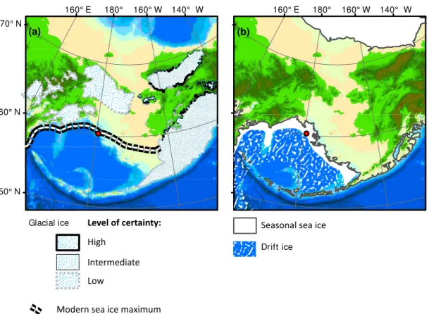
Figure 2.Maximum glacial and sea ice extents in Beringia. Panel(a)depicts the maximum glacial ice in Beringia as inferred from terminal and lateral moraines (Gualtieri et al., 2000; Heiser and Roush, 2001; Kaufman, et al., 2011; Barr and Clark, 2009). This is not intended to show the maximum extent during a particular glaciation but rather the maximum possible extent of glacial ice. These moraines are likely from several different major glaciations. The level of certainty is indicated by the thickness of the line at the moraine. The white-and-black dashed line is the maximum extent of sea ice (median over period 1979–2013) (Cavalieri et al., 1996). Panel(b)depicts the approximate pattern of sea ice during glacial stages (Katsuki and Takahashi, 2005). The dark-grey contour is−140 m a.p.s.l., the approximate sea level
during MIS 12 (Rohling et al., 2010). Base map is modified from Manley (2002).
East Siberian, Chukchi, and Beaufort seas (Fig. 1). On land, Beringia extends from the Lena River in Siberia to the Mackenzie River in Canada. Large portions of the Beringian shelf were exposed when sea level dropped below −50 m (Hopkins, 1959), and this subaerial expanse stretches more than 1000 km from north to south during most glacial periods (Fig. 2). In contrast, as sea level rises at glacial terminations, the expansive continental shelf is flooded rapidly once sea level reaches −60 m a.p.s.l. (Keigwin et al., 2006). This in-troduces fresh organic matter and nutrients into the southern Bering Sea (i.e., Bertrand et al., 2000; Shiga and Koizumi, 2000; Ternois et al., 2001), re-establishing at −50 m a.p.s.l. the connection between the Pacific and Atlantic oceans through Bering Strait (Keigwin et al., 2006). The late Ceno-zoic history of the depth of the Bering Strait sill is poorly known; hence, current oceanographic reconstructions (e.g., Knudson and Ravelo, 2015) assume that a sill depth of −50 m a.p.s.l. was temporally stable, which is probably not the case and requires future study. However, in this study, we also assume that a sill depth of −50 m a.p.s.l. controls
oceanographic communication between the Atlantic and Pa-cific oceans.
2.2 Site location and oceanographic setting
The Integrated Ocean Drilling Program’s (IODP) Expedition 323, Site U1345, is located on an interfluve ridge near the shelf-slope break in the Bering Sea (Fig. 1). Navarin Canyon, one of the largest submarine canyons in the world (Normack and Carlson, 2003), is located just to the northwest of the site. Sediments were retrieved from∼1008 m of water, plac-ing the site within the center of the modern-day oxygen min-imum zone (Takahashi et al., 2011). We focus on this site because of its proximity to the modern marginal ice zone in the Bering Sea and observed high sedimentation rates. Its sit-ing on top of an interfluve was chosen to reduce the influence of turbidites moving through Navarin Canyon.
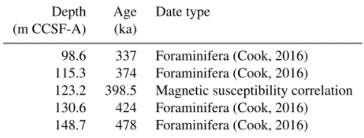
Table 1.Age–depth tie points used in the age model for U1345.
Depth Age Date type
(m CCSF-A) (ka)
98.6 337 Foraminifera (Cook, 2016)
115.3 374 Foraminifera (Cook, 2016)
123.2 398.5 Magnetic susceptibility correlation
130.6 424 Foraminifera (Cook, 2016)
148.7 478 Foraminifera (Cook, 2016)
Bering Sea through deep channels in the western Aleutian Islands. Once north of the Aleutian Islands, this water mass becomes the Aleutian North Slope Current (ANS), and flows eastward until it reaches the Bering Sea shelf. Interactions with the shelf turn this current to the northwest, where it becomes the Bering Slope Current (Stabeno et al., 1999). Tidal forces and eddies in the Bering Slope Current drive up-welling through Navarin Canyon and other interfluves along the shelf-slope break (Kowalik, 1999). The resulting cold wa-ter and nutrients brought to the sea surface, coupled with the presence of seasonal sea ice, drive the high productiv-ity found today in the so-called “Green Belt” (Springer et al., 1996) along the shelf-slope break. North of the site, low-salinity, high-nutrient shelf waters (Cooper et al., 1997) pri-marily flow north through the Bering Strait to the Arctic Basin (Schumacher and Stabeno, 1998).
3 Methods
3.1 Age model
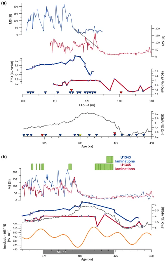
The age model (Fig. 3) is derived from the shipboard age model, which was developed using magnetostratigraphy and biostratigraphy. First and last appearance datums for diatoms and radiolarians make up the majority of the biostratigraphic markers used to place the record in the correct general strati-graphic position (Takahashi et al., 2011). Oxygen isotope measurements taken on the benthic foraminifera,Uvigerina peregrina,Nonionella labradorica, andGlobobulimina affi-nis(Cook et al., 2016) were then used to tune site U1345 to the global marine benthic foraminiferal isotope stack (LR04) (Lisiecki and Raymo, 2005) (Fig. 3; Table 1). Based on this combined age model, MIS 11 spans from 115.3 to 130.6 mbsf (Cook et al., 2016); however, the characteristic interglacial isotopic depletion was not found in U1345, which means that the exact timing of peak interglacial conditions is unknown.
The nearby core from Site U1343 of IODP Expedition 323 (Fig. 1) has an excellent oxygen isotopic record during MIS 11 (Asahi et al., 2016). We compared the two isotopic records and their magnetic susceptibilities (Fig. 3) and found that, even with only two tie points, there was good correla-tion between the timing of the onset of laminated intervals and also the interglacial increase in magnetic susceptibility (Fig. 3b). We added one additional tie point to connect the
in-flection points in magnetic susceptibility (Table 1). In U1343, this point occurred at 398.50 ka. U1345 was shifted 1.5 ka younger in order to align with U1343. The addition of this point allows us to have more confidence in the timing of peak interglacial conditions in U1345. However, given the oxygen isotope sampling resolution, as well as the stated error in the LR04 dataset (4 kyr), we estimate the error of the age model could be up to 5 kyr. Therefore, we urge caution when com-paring millennial-scale changes at this site with other sites that examine MIS 11 at millennial-scale resolution or finer.
Sedimentation rates during the study interval range from 29 to 45 cm kyr−1, with the highest sedimentation rates
oc-curring during glacial periods. Depths and ages of major cli-mate intervals referred to in the text are found in Table 2.
3.2 Sediment analyses
Details about sediment sampling can be found in the Sup-plement. Quantitative diatom slides were prepared (Scherer, 1994) and counted (Schrader and Gersonde, 1978) using published taxonomic descriptions and images (Hasle and Heimdal, 1968; Koizumi, 1973; Lundholm and Hasle, 2008, 2010; Medlin and Hasle, 1990; Medlin and Priddle, 1990; Onodera and Takahashi, 2007; Sancetta, 1982, 1987; Syvert-sen, 1979; Tomas, 1996; Witkowski et al., 2000). Diatom taxa were then grouped according to ecological niche (Ta-ble 3) based on biological observations (Aizawa et al., 2005; Fryxell and Hasle, 1972; Håkansson, 2002; Horner, 1985; Saito and Taniguchi, 1978; Schandelmeier and Alexander, 1981; von Quillfeldt, 2001; von Quillfeldt et al., 2003) and statistical associations (Barron et al., 2009; Caissie et al., 2010; Hay et al., 2007; Katsuki and Takahashi, 2005; Lopes et al., 2006; McQuoid and Hobson, 2001; Sancetta, 1982, 1981; Sancetta and Robinson, 1983; Sancetta and Silvestri, 1986; Shiga and Koizumi, 2000). In cases where a diatom species was reported to fit into more than one environmen-tal niche, it was grouped into the niche where it was most commonly recognized in the literature.
Eighteen quantitative calcareous nannofossil slides were prepared (Flores and Sierro, 1997) and counted using a Zeiss polarized light microscope at 1000×magnification. Samples were considered barren if no coccoliths were found in at least 165 randomly selected fields of view. All taxa were identified to the species or variety level (Flores et al., 1999; Young et al., 2003).
Grain size of both biogenic and terrigenous sediment was measured using a Malvern Mastersizer 3000 with the Hy-dro MV automated wet dispersion unit. The mineralogy of 10 samples was analyzed using a Siemens D-5000 X-ray diffractometer (Eberl, 2003).
0 5 4 5
2 4 0
0 4 5
7 3
Age (ka)
5 4.5 4 3.5 3
1
8O
(‰
VPDB)
0 50 100 150 200
MS
(SI)
460 470 480 490 500 510 520
In
so
la
io
n
(
6
5
° N
)
[W
m
]
-2
MIS 11
U1345 laminations
U1343
laminations 5.2
4.8 4.4 4 3.6 3.2
1
8O
(‰
VPDB)
5.2 4.8 4.4 4 3.6 3.2
1
8O
(‰
VPDB)
5.2 4.8 4.4 4 3.6 3.2
1
8O
(‰
VPDB)
0 50 100 150 200
MS
(SI)
0 50 100 150 200
MS
(SI)
0 5 4 5
2 4 0
0 4 5
7 3
Age (ka)
100 110 120 130 140
CCSF-A (m)
(a)
(b)
Figure 3.(a)Age model plotted by depth. Blue plots depict data from Site U1343, while red plots are from U1345. Magnetic susceptibility and benthic foraminiferalδ18O are plotted by depth for each site in the top half of the figure. The grey line joining the magnetic susceptibility
plots indicates the tie point that was added in this study. Inverted triangles indicate locations of tie points (red: U1345; blue: U1343; grey: magnetic susceptibility) between Bering Seaδ18O (Cook et al., 2016; Asahi et al., 2016) and the global marine stack (Lisiecki and Raymo,
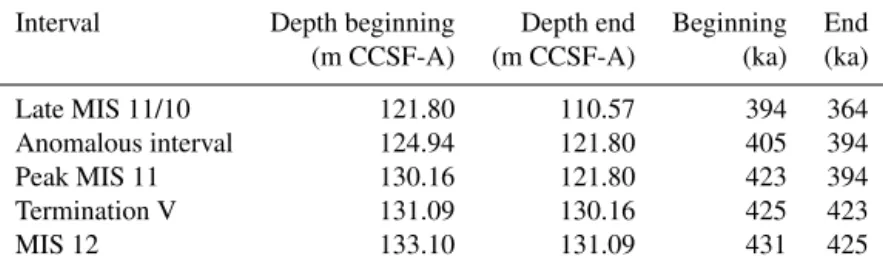
Table 2.Depths and ages of major climate intervals referred to in the text.
Interval Depth beginning Depth end Beginning End
(m CCSF-A) (m CCSF-A) (ka) (ka)
Late MIS 11/10 121.80 110.57 394 364
Anomalous interval 124.94 121.80 405 394
Peak MIS 11 130.16 121.80 423 394
Termination V 131.09 130.16 425 423
MIS 12 133.10 131.09 431 425
Table 3.Bering Sea diatom species grouped by environmental niche. In cases where a species appears in more than one niche, the grouping used in this study is highlighted in bold.
Modern seasonal succession
Epontic Marginal ice zone (MIZ) Both epontic and MIZ Summer bloom
Navicula transitrans Bacterosira bathyomphala Actinocyclus curvatulus Coscinodiscusspp.
Synedropsis hyperborea Chaetoceros furcellatus Fossula arctica Leptocylindrussp.
Chaetoceros socialis Fragilariopsis cylindrus Rhizosoleniaspp.
Leptocylindrussp. Fragilariopsis oceanica
Odontella aurita Fragilariopsis regina-jahniae
Paralia sulcata Navicula pelagica
Porosira glacialis Naviculoid pennates
Staurosirellacf.pinnata Nitzschiaspp.
Thalassionema nitzschioides Pinnularia quadratarea Thalassiosira angulata Thalassiosira antarcticaRS
Thalassiosira baltica Thalassiosira gravida
Thalassiosira decipiens Thalassiosira hyalina Thalassiosira hyperborea Thalassiosira nordenskioeldii
Thalassiosira pacifica
Water mass tracers Shelf to basin transport
Dicothermal High productivity Alaska stream Warmer water Neritic Fresh water
Actinocyclus curvatulus Chaetocerosspp. Neodenticula seminae Azpeitia tabularis Actinoptychus senarius Lindaviacf.ocellata Shionodiscus trifultus Odontella aurita Stellarimiastellaris Amphorasp. Lindavia stylorum
Thalassionema nitzschioides Thalassionema nitzschioides Lindavia stylorum Staurosirellacf.pinnata Thalassiosira pacifica Thalassiosira eccentrica Delphineisspp. Lindavia radiosa Thalassiosiraspp. small Shionodiscus oestrupii Detonula confervacea
Thalassiothrix longissima Thalassiosira symmetrica Diploneis smithii Naviculoid pennates Odontella aurita Paralia sulcata Rhaphoneis amphiceros Stephanopyxis turris Thalassiosira angulata Thalassiosira decipiens Thalassiosira eccentrica
Laboratory. The 1σprecision of stable isotope measurements and elemental composition of carbon is 0.2 ‰ and 0.03 %, respectively, and 0.2 ‰ and 0.002 %, respectively, for nitro-gen.δ13C values are reported relative to the Vienna Pee Dee
Belemnite (VPDB) andδ15N values are reported relative to
atmospheric N2. Percent CaCO3was calculated according to Schubert and Calvert (2001). More detailed methodology can be found in the Supplement.
4 Results
4.1 Sedimentology
or volcanogenic grains is highest during laminated intervals and lowest immediately preceding Termination V (∼425 ka). Vesiculated tephra shards were seen in every diatom slide an-alyzed. Several thin (< 1 cm) sand layers and shell fragments were visible on the split cores, especially during MIS 12. However, high-resolution grain size analyses show that the median grain size was lowest during MIS 12, increasing from approximately 14 to 21 µm at the start of Termination V at 424.5 ka (130.92 m b.s.f.). Median grain size peaks at 84 µm between 401 and 407 ka (125.42–123.62 m b.s.f.). This inter-val is also the location of an obvious sandy layer in the core. After this “anomalous interval”, median grain size remains steady at about 17 µm. Subrounded to rounded clasts (gran-ule to pebble) commonly occur on the split surface of the cores. We combined clast and sand layer data from all holes at Site U1345 when examining their distribution (Fig. 4).
A 3.5 m thick laminated interval, estimated to span 12 kyr (see Table 4 for depths and ages), is deposited beginning dur-ing Termination V. Although the termination is short-lived and the laminated interval quite long, we refer to it as the Termination V Laminations for the sake of clarity throughout this manuscript. The next laminated interval occurs at about 394 ka and lasts approximately 1.1 kyr. During the transition from late MIS 11 to MIS 10, a series of four thin laminated intervals are observed. Each interval lasts between 0.34 and 1.25 ka (Table 4). In general, the upper and lower boundaries of laminated intervals are gradational; however, the bound-aries between individual lamina are sharp (Takahashi et al., 2011). There are two types of laminations. The Termination V Laminations are type I laminations: millimeter-scale alter-nations of black, olive-grey, and light-brown triplets. In ad-dition to containing a high proportion of diatoms, this type of laminated interval also contains high relative proportions of calcareous nannofossils and foraminifera (Takahashi et al., 2011). The majority of laminations are parallel; how-ever, a 7 cm interval during the Termination V Laminations is highly disturbed in Hole A, showing recumbent folds in the laminations (Takahashi et al., 2011). This interval was not sampled. Type II laminations occur throughout the remain-der of MIS 11. These laminations have fewer diatoms and tend to be couplets of siliciclastic sediments with < 40 % di-atoms (Takahashi et al., 2011). Percent CaCO3also increases during these laminations though foraminifera and calcareous nannofossils are very rarely seen. None of these later lami-nated intervals contain any evidence of disturbance.
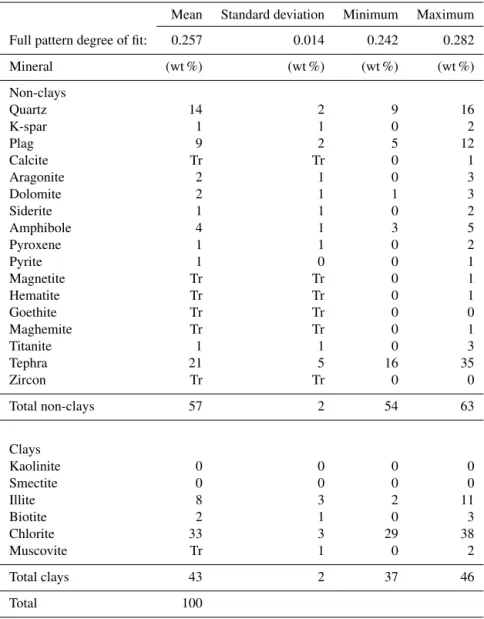
4.2 Mineralogy
We determined the weight percent of 23 common minerals in 10 samples across the study interval. Samples are primar-ily composed of quartz, plagioclase, tephra, illite, and chlo-rite with minor amounts of other clay and non-clay miner-als (Table 5). Downcore, the largest variability occurs in the weight percent of quartz, chlorite, and illite. In general, chlo-rite comprises nearly 35 % of the minerals present in the
sedi-440 430 420 410 400 390 380 370
Age
(k
a
BP)
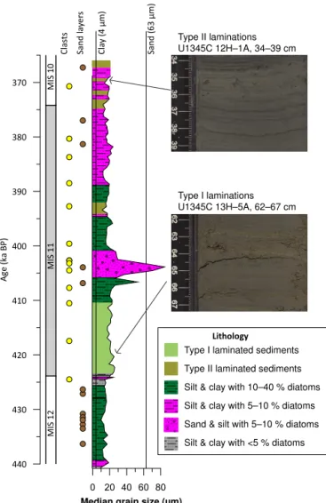
0 20 40 60 80
Median grain size (µm)
Lithology
Type I laminated sediments
Silt & clay with 5–10 % diatoms
Sand & silt with 5–10 % diatoms Silt & clay with 10–40 % diatoms
Silt & clay with <5 % diatoms
Clas
ts
Sand la
y
er
s
Sand (63
µm)
Cla
y (4
µm)
MIS 11
Type II laminated sediments Type I laminations
U1345C 13H–5A, 62–67 cm Type II laminations U1345C 12H–1A, 34–39 cm
MIS 10
MIS 12
Figure 4.Lithostratigraphic column for U1345A. Marine Isotope Stage 11 is depicted as a grey bar. Ice-rafted debris (yellow dots) and sand layers (brown dots) are a compilation of these features in all four holes at U1345. The width of the lithologic column varies according to median grain size. Vertical lines indicate the cut-off for clay- and sand-sized particles. Silt lies between the two lines. Colors depict varying amounts of diatoms relative to terrigenous grains in the sediment. Type I laminations are depicted as pale-green bars and type II laminations are depicted as olive-green bars. An example of each of the lamination types is shown in the images to the right.
Table 4.Distribution of laminated intervals during MIS 11. Note that the depth and age of laminated intervals encompasses all holes drilled, but the median duration is calculated using each of the holes that it is present in.
Lamination Type Depth Age Median Found
duration in holes
(mbsf) (ka) (kyr)
MIS 11.5 II 112.02–111.47 367.23–366.00 0.51 CDE
MIS 11.4 II 113.14–112.94 369.72–369.26 0.34 CD
MIS 11.3 II 114.28–113.95 372.25–371.52 0.73 D
MIS 11.2 II 115.59–114.69 374.75–373.17 1.23 ACE
MIS 11.1 II 121.84–121.18 394.12–392.09 1.10 CE
Termination V I 130.23–126.51 423.28–410.44 12.04 ACDE
4.3 Diatoms
4.3.1 Diatom assemblages
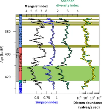
A total of 97 different diatom taxa were identified. Individ-ual samples include between 26 and 46 taxa each with an average of 37 taxa. Both types of laminated intervals con-tain fewer taxa than bioturbated intervals do. This decrease in diversity is confirmed using the Margalef, Simpson, and Shannon indices (Maurer and McGill, 2011), which all show similar downcore profiles (Fig. 5). The Margalef index is a measure of species richness. It shows a decrease in the num-ber of taxa during four out of five laminated intervals that are sufficiently well sampled. Between laminated intervals, there is also a noted decrease in taxa at 388 ka. The Simpson index measures the evenness of the sample. Values close to 1 indicate that all taxa contain an equal number of individ-uals, while values close to 0 indicate that one species domi-nates the assemblage. In general, the Simpson index is close to 1 throughout the core; however, during the Termination V Laminations and the most recent two laminations, the Simp-son index decreases reflecting the dominance byChaetoceros resting spores (RS) during these intervals (Fig. 5). The Simp-son index never approaches 0, which would likely indicate a strong dissolution signal. The Shannon diversity index mea-sures both species richness and evenness. Correspondingly, it is low during three of the laminated intervals and high during MIS 12, and peaks at 397 ka (Fig. 5).
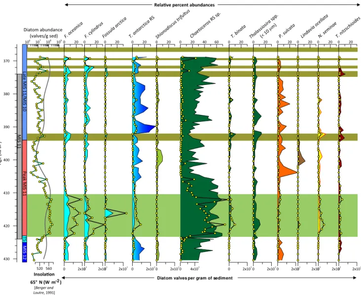
Absolute diatom abundances vary between 106 and 108 diatoms deposited per gram of sediment with values an or-der of magnitude higher during most laminated intervals than during massive intervals (Fig. 5). The diatom assemblage is dominated by Chaetoceros andThalassiosira antarctica RS, with lesser contributions fromFragilariopsis oceanica, F. cylindrus,Fossula arctica,Shionodiscus trifultus(=T. tri-fulta),T. binata, small (< 10 µm in diameter)T. species, Par-alia sulcata, Lindavia cf. ocellata, Neodenticula seminae, andThalassionema nitzschioides(Fig. 6).
420 400 380
Age
(k
a
BP)
0.5 0.75 1
Simpson index
2 3 4
Shannon diversity index
106 107 108 109
Diatom abundances (valves/g sed)
4 5 6 7 8
M argalef index
MI
S
1
1
T
5
MI
S
1
2
Pe
ak
MIS
11
Late
MI
S
11
/MI
S
1
0
Figure 5.The Margalef, Simpson, and Shannon diversity indices plotted with diatom abundances. Type I laminations are depicted as pale-green bars and type II laminations are depicted as olive-green bars. Colored vertical bars refer to the zones mentioned in the text.
4.3.2 Qualitative diatom proxies
Table 5.Summary statistics for X-ray diffraction.
Mean Standard deviation Minimum Maximum
Full pattern degree of fit: 0.257 0.014 0.242 0.282
Mineral (wt %) (wt %) (wt %) (wt %)
Non-clays
Quartz 14 2 9 16
K-spar 1 1 0 2
Plag 9 2 5 12
Calcite Tr Tr 0 1
Aragonite 2 1 0 3
Dolomite 2 1 1 3
Siderite 1 1 0 2
Amphibole 4 1 3 5
Pyroxene 1 1 0 2
Pyrite 1 0 0 1
Magnetite Tr Tr 0 1
Hematite Tr Tr 0 1
Goethite Tr Tr 0 0
Maghemite Tr Tr 0 1
Titanite 1 1 0 3
Tephra 21 5 16 35
Zircon Tr Tr 0 0
Total non-clays 57 2 54 63
Clays
Kaolinite 0 0 0 0
Smectite 0 0 0 0
Illite 8 3 2 11
Biotite 2 1 0 3
Chlorite 33 3 29 38
Muscovite Tr 1 0 2
Total clays 43 2 37 46
Total 100
niche show differing abundance patterns over time. On the other hand, changes in abundances may simply reflect differ-ent species filling the same niche at differdiffer-ent times.
Chaetoceros RS are the dominant taxa included in the high-productivity group (Table 3). Relative percent abun-dances of Chaetoceros RS are highest (up to 69 %) during the Termination V Laminations and follow the pattern of both diatom accumulation rate (Fig. 7c) and insolation at 65◦N (Berger and Loutre, 1991). The lowest relative
abun-dances (15–20 %) of Chaetoceros/high-productivity species occur between 403 and 390 ka (124.21 to 120.07 m b.s.f.), when both obliquity and insolation are low (Fig. 7h).
Epontic diatoms are those that bloom attached to the un-derside of sea ice or within brine channels in the ice (Alexan-der and Chapman, 1981). This initial bloom occurs below the ice as soon as enough light penetrates to initiate photosyn-thesis in the Bering Sea, which can occur as early as March
(Alexander and Chapman, 1981). A second ice-associated bloom occurs as sea ice begins to break up on the Bering Sea shelf. This bloom is referred to as the marginal ice zone bloom and many of its members are common species in the sediment assemblage. Several diatom species are present in both types of sea ice blooms, and so while they are indicators of ice presence, they cannot be used to distinguish between types of sea ice. These species are grouped under “both ice types” (Table 3).
430 420 410 400 390 380 370
Age
(ka BP)
0 20
F. o cean
ica
0 20
T. n itzsc
hioi des
0 20
T. a ntar
ctica RS
0 20 Shio
nodi scus
trifu ltus
0 20 Thal
assio sira
spp.
(< 1 0 m
)
0 20 N. se
min ae
0 20
Linda via oc
ella ta
0 20 T. b
inat a
0 20
P. su lcata
0 20 40 60
Chae toce
ros RS sp
.
0 20
F. cy lindr
us
0 20
Foss ula
arct ica
520 560 Insolaion
65° N (W m ) -2 [Berger and Loutre, 1991] 106
107 108
109
Diatom abundance (valves/g sed)
0 2x10⁷ 0 2x10⁷ 0 2x10⁷
0 4x10⁷
0 2x10⁷ 0 2x10⁷
0 2x10⁷ 0 2x10⁷
0 2x10⁷ 0 2x10⁷ 0 2x10⁷
0 2x10⁷
Relaive percent abundances
Diatom valves per gram of sediment
MIS 11
T
5
MIS 12
Pe
ak MIS 11
La
te
MI
S
11
/MI
S
1
0
Figure 6.Absolute and relative percent abundances of all diatoms that occur in abundances greater than 10 % of any assemblage. Colored vertical bars refer to the zones mentioned in the text. Line plots depict absolute abundance and area plots depict relative percent abundance. Species are color-coded according to the niche that they are grouped into: marginal ice zone (light blue), both ice types (dark blue to light blue), dicothermal (light green), high productivity (green), neritic (orange), freshwater (brown), North Pacific (yellow), and warm water (red). Insolation at 65◦N (light-grey line) is also shown. Type I laminations are depicted as pale-green bars and type II laminations are depicted as olive-green bars.
A cold layer of water found between seasonally warmer surface and warmer deep water characterizes dicothermal water. It is stable because of its very low salinity. In the Sea of Okhotsk and the Bering Sea today, the dicothermal layer is associated with melting sea ice. Genera present in the Bering Sea during late summer tend to covary with the dicothermal water indicators, so the two groups were merged for com-parison with other diatom groups.S. trifultusis the dominant species in the dicothermal group (Table 3). It is relatively high (∼4 %) during MIS 12, is virtually absent from the sediments during the Termination V Laminations, and then increases again until it peaks at 10 % relative abundance at 400 ka (123.22 m b.s.f.) (Fig. 6).
Neritic species maintain ∼10 % relative abundance throughout the core (Fig. 7m). The dominant species in the neritic group isParalia sulcata (Table 3), sometimes con-sidered an indicator of shallow, moving water (Sancetta, 1982). Neritic species are lowest during the Termination V Laminations and increase dramatically around 404 ka (124.61 m b.s.f.) to almost 50 % of the assemblage (Fig. 7n).
L. cf. ocellata is the dominant taxa in the freshwater group. This group is notably absent from much of the core but prevalent between 401 and 392 ka (123.70 m b.s.f. and 121.20 m b.s.f.); it reaches its highest relative percent abun-dance (12 %) at 401 ka (123.62 m b.s.f.) (Fig. 7n).
430 420 410 400 390 380 370
Age
(k
a
BP)
0 20 40 60 Upwelling/ Chaetoceros
0 20 N. seminae
0 Warmer
water 0 20
Fresh water 0 Neriic20 40
0 20
Summer &
dicothermal
106 107 108
109
Diatom
valves /g sed
420 440 460 Insolaion
65° N (W m )-2 [Berger and Loutre, 1991]
-120 -80 -40 0 Relaive sea level (mapsl) [Rohling et al., 2009]
0.5 1 1.5 TOC % U1345
3 4 5 6 7 8 9
15N bulk
(‰vs air) * 8 C/N*
-28 -26 -24 -22
13C ‰ *
0 104 Calcareous nannofossils
(per gram sediment)
0 1 2 3 4
CaCO3%
0 20
Eponic
0 20 M arginal
icezone
0 20 40 Both ice types
MI
S
1
1
Relative percent abundances of niche groupings
T
5
MI
S
1
2
Peak
MIS
11
Late
MI
S
11
/MI
S
1
0
a b c d e f g h i j k l m n o p
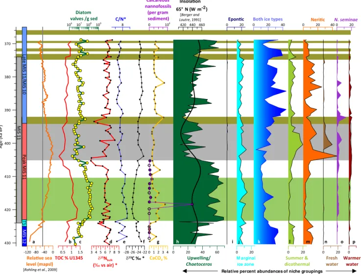
Figure 7.Summary of geochemistry and biological proxies. The grey vertical bar depicts the duration of MIS 11 and colored vertical bars refer to the zones mentioned in the text.(a)Global eustatic sea level (orange) is plotted for reference (Rohling et al., 2010). The sill depth of Bering Strait (−50 m a.p.s.l.) is shown as a vertical grey line. Total organic carbon (b, red) is plotted with the total diatom abundance (c, green line, yellow dots). Geochemical data are plotted asδ15N (d, red), C/N (e, blue),δ13C (f, black), and %CaCO3(g, yellow). Biological proxies include absolute abundance of calcareous nannofossils (g, purple). Open circles indicate barren samples; closed circles indicate samples that had calcareous nannofossils present. Relative percent abundances of diatoms are grouped by environmental niche.Chaetoceros
RS are green(h), epontic species are navy blue(i), marginal ice zone species are light blue(j), species that fall under both ice categories are shaded with a gradational blue(k), summer and dicothermal species are light green(l), neritic species are orange(m), freshwater species are brown(n),N. seminaeis purple(o), and warmer water species are maroon(p). Insolation at 65◦N (black) is overlain onChaetocerosRS relative percent abundances. Type I laminations are depicted as pale-green bars and type II laminations are depicted as olive-green bars. A grey bar indicates the anomalous interval.
2005). Absolute abundances begin to increase at 422 ka as global eustatic sea level rises above −50 m a.p.s.l. Abun-dance then decreases slowly over the course of the Termi-nation V LamiTermi-nations and peaks again at 392 and 382 ka. As sea level drops below −50 m a.p.s.l., N. seminae is no longer present at U1345. Relative percent abundances re-main stable at∼2 % relative percent abundance between 422 and 400 ka (129.62–123.62 m b.s.f.) and then peak at 13 % at 392 ka (121.22 m b.s.f.) (Figs. 6 and 7o).
Diatoms associated with warmer water or classified as members of temperate to subtropical assemblages (Table 3)
are quite low throughout the record (< 5 %), and are highest (3–4 %) during mid- to late MIS 11 at approximately∼410 to 391 ka (126.74–116.50 m b.s.f.) (Fig. 7p).
4.4 Calcareous nannofossils
midway through the Termination V Laminations when the di-atom assemblage is overwhelmingly dominated by Chaeto-cerosRS. SmallGephyrocapsa dominates (> 50 %) the cal-careous nannofossil assemblage. There are 35 % medium Gephyrocapsa, 9 %Coccolithus pelagicus, and 1 % Gephy-rocapsa oceanica.
4.5 Geochemistry
4.5.1 Organic and inorganic carbon content
Total organic carbon (TOC) roughly follows the trend of rela-tive percent abundances ofChaetocerosRS, with higher val-ues during the Termination V Laminations (Fig. 7b, 7h). The mean TOC value during MIS 12 is 0.76 %, and during the Termination V Laminations it is 1.11 %. TOC decreases be-tween 408 (125.82 m b.s.f.) and 404 ka (124.77 m b.s.f.), co-eval with a decrease inδ15N values. After 404 ka, it increases linearly to 374 ka (115.39 m b.s.f.). TOC is again high during the late MIS 11/MIS 10 laminations.
In contrast, inorganic carbon, calculated as % CaCO3, is less than 1 % for most of the record (Fig. 7g). However, it in-creases up to 3.5 % during the laminated intervals and also at 382 ka (117.87 m b.s.f.), 392 ka (110.00 m b.s.f.), and 408 ka (125.82 m b.s.f.).
4.5.2 Terrigenous vs. marine input indicators
Nitrogen, carbon, and their isotopes can be used to determine relative amounts of terrigenous vs. marine organic mater in-put. Total nitrogen (TN) is significantly correlated with total organic carbon (TOC) (Fig. 8a); however, they intercept of
a regression line through the data is 0.03 (Fig. 8a), indicat-ing that there is a significant fraction of inorganic nitrogen in the sediments (Schubert and Calvert, 2001). Inorganic nitro-gen can be adsorbed onto clay particles or incorporated into the crystal lattice of potassium-rich clays such as illite. This complicates interpretations of elemental nitrogen and its iso-topes because the presence of inorganic nitrogen will lower Corg/N ratios andδ15N values (Muller, 1977; Schubert and Calvert, 2001).
Bearing this bias in mind, the relative terrigenous contri-bution to the sediments can be estimated by examining where U1345 samples plot in relation to typical Corg/N,δ15N, and
δ13C values for marine phytoplankton, refractory soil organic
matter, and C3 vascular plants (Fig. 8). Note that we use N/Corg, the inverse of Corg/N, because we seek to derive
the terrigenous carbon fraction rather than the fraction of ter-rigenous nitrogen (Perdue and Koprivnjak, 2007). Through-out MIS 12–10, organic matter is comprised of a mixture of marine and terrigenous organic matter. There is a higher con-tribution of marine organic matter during MIS 12, 10, and between 394 and 405 ka, as well as a higher contribution of terrigenous organic matter during peak MIS 11 (Fig. 8). The N/Corgratio indicates that, during peak MIS 11, this
terrige-nous organic matter is likely refractory soil organic matter, rather than fresh vascular plant organic matter (Fig. 8b).
During MIS 12, Corg/N is highly variable, when sea level
is below−50 m a.p.s.l. (Fig. 7). As sea level rises during Ter-mination V, Corg/N values increase from 6 to more than 9. The highest Corg/N value occurs at the start of the Termina-tion V LaminaTermina-tions. Corg/N decreases as sea level rises until at 400 ka (123.62 m b.s.f.) it stabilizes near 7 for the remain-der of the record (Fig. 7).
Carbon isotopic values range between−22 and−26 ‰. No sample has high enough δ13C values to be comprised fully of typical Arctic Ocean marine phytoplankton (−22 to−19 ‰) or ice-related plankton (−18.3 ‰) (Schubert and Calvert, 2001); however, samples from MIS 10, MIS 12, and the “anomalous interval” all plot close to marine phy-toplankton values (Fig. 8b). At the onset of the Termination V Laminations,δ13C becomes more negative and then
grad-ually increases to a maximum of−22.33 at 404 ka (124.62). After 400 ka (123.5 m b.s.f.),δ13C is relatively stable around −23.5 ‰ (Fig. 7).
4.5.3 Nitrogen isotopes
The nitrogen isotopic composition of bulk marine sediments can be thought of as a combination of theδ15N of the source nitrate and the amount of nitrogen utilization by phytoplank-ton (Brunelle et al., 2007). Denitrification is common in the low-oxygen waters of the eastern tropical North Pacific (Liu et al., 2005) and in the Bering Sea during the Bølling–Allerød (Schlung et al., 2013), leading to enriched core-top δ15N
values between 8 and 9 ‰. When diatoms utilize nitrogen, they preferentially assimilate the lighter isotope,14N, which enriches surface waters with respect to15N (Sigman et al., 1999). Complete nitrogen utilization would result in δ15N
values identical to that of the source nitrate (Sigman et al., 1999). Sponge spicules (very lowδ15N values) and radiolar-ians (highly variableδ15N values) may contaminate theδ15N of bulk organic matter; therefore, we looked for and found no correlation between spicule abundance andδ15N in our samples.
δ15N is relatively stable but quite high throughout the study interval, fluctuating around an average value of 6.4 ‰ and reaching values greater than 7 ‰ and up to 8 ‰ sev-eral times (Fig. 7). There are sevsev-eral notable excursions from these high values. Coeval with sea level rise and in-creased relative percent Chaetoceros RS, δ15N decreased
-20 -22 -24 -26 13C ‰ *
0 0.04 0.08 0.12 0.16 0.2
N
C
-20 -22 -24 -26
13C ‰ * 0
2 4 6 8 10
1
5N
bul
k
(
‰
v
s.
a
ir
)
*
0 0.4 0.8 1.2 1.6
Total organic carbon 0
0.04 0.08 0.12 0.16 0.2
T
o
ta
l
n
it
ro
g
e
n
MIS 12 Terminaion V Peak MIS 11
MIS 10
Anomalousinterval y = 0.0922x + 0.0338
r2= 0.59
Marine phytoplankton
Marine phytoplankton
Soil/ vascular plants
Vascular plants Soil (a)
(c)
(b)
-1
Figure 8.Cross plots of(a)total nitrogen vs. total organic carbon,(b)N/Corgvs.δ13C, and(c)δ15N vs.δ13C. For each panel, the range of composition of each organic matter source is plotted in a grey box: marine phytoplankton (C/N: 5–7 – Redfield, 1963; Meyers, 1994;
δ13C:−19 to−22 ‰ – Schubert and Calvert, 2001;δ15N: 5 to 8 ‰ – Walinsky et al., 2009); Soil (C/N: 10–12,δ13C:−25.5 to−26.5 ‰, δ15N: 0 to 1 ‰ – Walinsky et al., 2009); C3 vascular plants (C/N: > 20 – Redfield, 1963; Meyers, 1994;δ13C:−25 to−27 ‰ – Schubert
and Calvert, 2001;δ15N: 0 to 1 ‰ – Walinsky et al., 2009).
5 Discussion
5.1 Orbital-scale changes in productivity and sea ice The observed changes in diatom assemblages and lithology (Fig. 7) allow us to break the sedimentary record into five zones: MIS 12, Termination V, peak MIS 11, anomalous in-terval, and late MIS 11 (Table 2). These zones reflect chang-ing sea ice, glacial ice, sea level, and sea surface temperature (SST) and correspond to events recognized elsewhere in ice cores and marine and lake sediments.
5.1.1 Marine Isotope Stage 12 and early deglaciation (431–425 ka)
N/Corg) and isotopic (δ13C,δ15N) indicators of terrigenous
and marine carbon pools indicate that the organic matter dur-ing MIS 12 is a diverse mix of marine phytoplankton and soil detritus (Fig. 8) likely derived from in situ, but low, pro-ductivity and transport by several methods including large, oligotrophic rivers and downslope transport. Glacial ice was likely restricted to mountain-valley glaciers, similar to the Last Glacial Maximum (e.g., Glushkova, 2001). These small, distant glaciers would not have produced large amounts of icebergs though occasional glacial IRD may have come from the Koryak Mountains, the Aleutians, or Beringia. Consistent with this, sediments typical of glacial IRD, such as drop-stones, are sparse but present. In addition, sea ice rafting tends to preferentially entrain clay and silt (Reimnitz et al., 1998) and is likely to be an important contributor of terrige-nous sediments.
5.1.2 Termination V (425–423 ka)
Termination V is the transition from MIS 12 to MIS 11. Worldwide, it is a rapid deglaciation that is followed by a long (up to 30 kyr) climate optimum (Milker et al., 2013). At U1345, gradually increasing productivity coupled with decreasing nutrient utilization and sea ice occurs between 425 and 423 ka. This is seen as an increase in absolute di-atom abundances and relative percent abundance of Chaeto-ceros RS and a decrease in sea ice diatoms andδ15N
val-ues (Fig. 7). It is plausible that increased nitrogen availability drove higher primary productivity as floods scoured fresh or-ganic matter from the submerging continental shelf (Bertrand et al., 2000). Rapid input of bioavailable nitrogen as the shelf was inundated has been suggested to explain increasing pro-ductivity during the last deglaciation in the Sea of Okhotsk (Shiga and Koizumi, 2000) and during MIS 11 in the North Atlantic (Poli et al., 2010) and also may have contributed to dysoxia by ramping up nutrient recycling, bacterial respira-tion, and decomposition of organic matter in the Bering Sea.
5.1.3 Peak MIS 11 (423–394 ka)
Globally, peak interglacial conditions (often referred to as MIS 11.3 or 11c) are centered around 400 to 410 ka (Dut-ton et al., 2015; Raymo and Mitrovica, 2012), though the ex-act interval of the temperature optimum varies globally and lasted anywhere from 10 to 30 kyr (Kandiano et al., 2012; Kariya et al., 2010; Milker et al., 2013). At U1345, peak in-terglacial conditions begin during the Termination V Lam-inations at 423 ka and continue until 394 ka, lasting nearly 30 kyr, consistent with the synthesis of the PAGES Past In-terglacials Working Group (2016).
Laminations (423–410 ka)
A 3.5 m thick laminated interval is deposited during early MIS 11, beginning at 423 ka (Fig. 7), when insolation was
high at 65◦N (Berger and Loutre, 1991). Its presence
indi-cates that the bottom water at 1000 m in the Bering Sea was dysoxic for more than 12 kyr. These laminations are char-acterized as type I laminations with a high diatom content (Fig. 4). Several lines of evidence point towards high produc-tivity among multiple phytoplankton groups as opposed to simply a change in preservation. First, we see an increase in diatom abundances by 2 orders of magnitude increase since MIS 12; second, a low-diversity diatom assemblage domi-nated byChaetocerosRS; third, an abrupt increase in percent organic carbon; and fourth, high percent CaCO3 and abun-dant calcareous nannofossils dominated by small Gephyro-capsa. Furthermore, enrichedδ15N values indicate either
in-creased nitrogen utilization that likely led to this inin-creased productivity or localized denitrification in low-oxygen wa-ters (Fig. 7).
Sea ice extent decreases during this interval, with no epon-tic diatoms present and reduced amounts of sea ice diatoms found in both epontic and marginal ice (Fig. 7). Geochem-ical cross plots indicate a high contribution from soil de-tritus and C3 plant organic matter (Fig. 8). At the onset of the laminated interval (423 ka),δ13C decreases and Corg/N increases rapidly (Fig. 7) as the tundra-covered Bering Sea shelf is flooded.
However, the diatom record during the laminated interval has the lowest contribution of neritic diatoms and virtually no freshwater diatoms (Fig. 7), suggesting that although ter-rigenous organic matter was an important input at the site, coastal, river, or swamp/tundra diatoms were not carried out to U1345 with this terrigenous organic matter.
Post-laminations (410–394 ka)
Both high N/Corgandδ13C indicate that input of terrigenous
430 420 410 400 390 380 370
Age
(k
a
BP)
0 20 40 Upwelling/
Chaetoceros
0 20
S. trifultus 0 8 16
Opal (wt %) U1345
0 20 40 All sea ice
diatoms 10 20 30
Opal (wt %) U1343
0 20 40 60 Opal (wt %)
U1341
-80 0
0 0.4 Δδ13C
U1342-849
24 32 40 Chlorite (wt %)
32 40 48 Illite (wt %)
U1343
0 4 8 12 Illite (wt %)
U1345
MI
S
1
1
T
5
M
IS
1
2
Peak
MIS
11
Late
MI
S
11
/MI
S
1
0
N
. A
tla
n
tic
st
a
d
ia
ls
I
II
III
IV
Weaker NPIW vent ilat ion
U1345
U1343
Figure 9.Comparison of Site U1345 with other Bering Sea (U1340, U1341, U1343) and global sites. The grey vertical bar depicts the duration of MIS 11, colored vertical bars refer to the zones mentioned in the text, and dark-grey bars show the timing of North Atlantic stadials (I–IV) (Voelker et al., 2010). Global eustatic sea level (orange) is plotted for reference (Rohling et al., 2010). The sill depth of Bering Strait (−50 m a.p.s.l.) is shown as a vertical grey line. Weight % opal from sites U1345, U1343, and U1341 (Kanematsu et al., 2013) is
plotted withChaetocerosRS relative percent abundances, and relative percent abundances of all sea ice diatoms. The difference in benthic foraminiferalδ13C between the Bowers Ridge (U1342) and the North Pacific (ODP 849), a proxy for North Pacific Intermediate Water ventilation, is plotted with relative percent abundances ofShionodiscus trifultus, an indicator of highly stratified water. Note that ventilation increases to the left. The weight percent of the clay minerals, chlorite, and illite are plotted for sites U1343 (Kim et al., 2015) and U1345 (this study). Type I laminations are depicted as pale-green bars and type II laminations are depicted as olive-green bars. A grey bar indicates the “anomalous interval”.
5.1.4 Late MIS 11 to MIS 10 (younger than 394 ka) After 394 ka, diatom productivity indicators are the lowest in the record but linearly increase to the top of the record. This is in contrast to a slight increase in diatom abundance, which increases at 393 ka and then remains relatively stable into MIS 10. Sea ice indicators also remain relatively high from 392 to the top of the record and dicothermal species reflect moderately stratified waters. Warm water species de-crease from 390 ka to the top of the record (Fig. 7). The sum of this evidence indicates that, at the end of MIS 11, summers were warm and sea ice occurred seasonally, perhaps lasting a bit longer than at other times in the record.
Eustatic sea level decreased beginning about 402 ka (Rohling et al., 2010), but sea level remained high enough to allowN. seminaeto reach the shelf slope break until about 380 ka (Fig. 7).
5.2 The Bering Sea in the context of regional and global variability
Biogenic opal increases during early MIS 11 at sites U1343 and U1345 (Kanematsu et al., 2013). At U1345, it mimics the pattern of relative percent abundance of Chaeto-cerosRS, the most abundant productivity indicator (Fig. 9). Although diatom data from other cored sites are low reso-lution (1–4 samples during MIS 11) (Kato et al., 2016; On-odera et al., 2016; Stroynowski et al., 2015; Teraishi et al., 2016), they provide a snapshot of diatom assemblages dur-ing MIS 11. Sea ice diatoms contribute approximately 30 % of the diatom assemblages at the two slope sites, U1345 (this study) and U1343 (Teraishi et al., 2016), and between 10 and 20 % of the assemblage at the eastern Bowers Ridge site (U1340) (Stroynowski et al., 2015), but less than 2 % of the assemblage on the western flanks of Bowers Ridge (U1341) (Onodera et al., 2016). In the North Pacific (ODP Site 884), no sea ice diatoms are present during MIS 11 (Kato et al., 2016). Site U1341 contained an assemblage high in dicother-mal indicators such as Shionodiscus trifultusand Actinocy-clus curvatulus, oceanic front indicators such as Rhizosole-nia hebetata, and N. seminae(Onodera et al., 2016), while the North Pacific (Site 884) assemblage is dominated by di-cothermal indicators during MIS 11 (Kato et al., 2016). Per-cent opal declines at Bowers Ridge during early MIS 11 at the same time as it increases at the slope sites (Iwasaki et al., 2016) (Fig. 9) when sea ice is reduced and upwelling along the shelf-slope break is increased. This implies that the rela-tionship between productivity and sea ice in the Bering Sea is perhaps more complex than the simple idea that sea ice inhibits productivity (Iwasaki et al., 2016; Kim et al., 2016). The region is strongly influenced by winter sea ice through-out MIS 11, with seasonal sea ice present farther sthrough-outh along the slope than today and also in the eastern Bering Sea. Highly stratified waters, perhaps due to the seasonal expan-sion and retreat of sea ice, extended across the entire basin and even into the North Pacific.
Local ventilation of North Pacific Intermediate Water de-creased as the Bering Strait opened during Termination V with the weakest ventilation occurring around 400 ka (Knud-son and Ravelo, 2015). This is coeval with the highest rel-ative percent abundances of dicothermal diatoms, indicating highly stratified water (Fig. 9).
5.2.1 Temperature and aridity during MIS 11
When sea level was low during glacial periods such as MIS 12 (Rohling et al., 2010), U1345 was proximal to the Beringian coast (Fig. 2). With the Bering land bridge ex-posed, the continent was relatively cold and arid (Glushkova, 2001). In western Beringia, Lake El’gygytgyn was perenni-ally covered with ice, summer air temperatures were warm-ing in sync with increaswarm-ing insolation from 4 to 12◦C, but
annual precipitation was low (200–400 mm) (Vogel et al., 2013).
As sea level rose, and global ice volume reached the lowest amount for the past 500 kyr (Lisiecki and Raymo,
2005), the generally continental temperatures in the Northern Hemisphere increased (D’Anjou et al., 2013; de Vernal and Hillaire-Marcel, 2008; Lozhkin and Anderson, 2013; Lyle et al., 2001; Melles et al., 2012; Pol, 2011; Prokopenko et al., 2010; Raynaud et al., 2005; Tarasov et al., 2011; Tzedakis, 2010; Vogel et al., 2013), with a northward expansion of bo-real forests in Beringia (Kleinen et al., 2014). However, the marine realm does not reflect this warming as strongly. At U1345, the relative percent of warm-water species suggests that SSTs during peak MIS 11 were only slightly warmer than during MIS 12. Indeed, MIS 11 is not the warmest in-terglacial in most marine records (Candy et al., 2014); rather, MIS 5e is the warmest in many places (PAGES Past Inter-glacials Working Group, 2016). This is especially evident in the Nordic Seas, where MIS 11 SSTs were lower than Holocene values (Bauch et al., 2000). However, MIS 11 is unique because it was much longer than MIS 5e in all records (PAGES Past Interglacials Working Group, 2016). One ex-ception to this is the Arctic Ocean, which was warm enough during MIS 11 to imply increased Pacific water input through Bering Strait (Cronin et al., 2013).
With elevated sea level, peak MIS 11c was very humid in many places. In the Bering Sea, modeling studies esti-mate up to 50 mm more precipitation than today at 410 ka (Kleinen et al., 2014). The most humid, least continental pe-riod recorded in the sediments at Lake Baikal occurs from 420 to 405 ka (Prokopenko et al., 2010), and extremely high precipitation is recorded at Lake El’gygytgyn on the nearby Chukotka Peninsula from 420 to 400 ka (Melles et al., 2012).
5.2.2 Millennial-scale laminations and changes in sea ice
Globally, late MIS 11 is characterized as a series of warm and cold cycles (Candy et al., 2014; Voelker et al., 2010), though there is no agreement on the timing of these cycles. At Site U1345, laminations are deposited intermittently between 394 and 392 ka and again after 375 ka (Fig. 4) as the climate tran-sitioned into MIS 10. These laminations are quite different from the Termination V Laminations due to their shorter du-ration and lack of obvious shift in terrigenous vs. marine car-bon source. In addition, these type II laminations have higher diatom abundances and CaCO3, but lack increased upwelling indicators. Primary production during these laminations is likely not driven by nutrient upwelling along the shelf-slope break. Instead, most of these laminations show an increase in sea ice diatoms and roughly correspond to millennial-scale stadial events that occurred during late MIS 11 in the North Atlantic (Fig. 9) (Voelker et al., 2010) as well as carbonate peaks at Blake Ridge (Chaisson et al., 2002). This suggests teleconnections between the Bering Sea and the North At-lantic at this time and places an indirect constraint on the depth of the Bering Strait sill.
430 420 410 400 390 380 370
Age
(k
a
BP
)
0 10 20 30
P. sulcata
0 10
Fresh water
106 107
108 40 60 80
Silt vol % 0 4 8 12 16 Clay vol %
4 6 8
15N (
bulk ‰vs. air) * 6 7 8 9 10
C/N*
-26 -24 -22 13C ‰ * 0 20 40 60
Sand vol %
0 4 8 12 16 150–250 μm vol %
0 2 4 6 8 > 250 μm vol %
0 2x10⁶ 0 2x10⁶
Clasts Relaive % abundance
Diatom valves/g Sed
Sand
MI
S
1
1
Anomalous int erval
Late
MIS
11/MIS
10
Pe
ak
MIS
11
T5
MI
S
1
2
Figure 10.Proxy indicators of shelf to basin transport. The grey vertical bar depicts the duration of MIS 11; colored vertical bars refer to the zones mentioned in the text. Total diatom absolute abundances are plotted next to absolute (line plots) and relative percent abundance ofP. sulcata(orange area plot) and freshwater species (brown area plot). High-resolution grain size includes % clay (red), silt (black), sand (red),
150–250 µm (black) and greater than 250 µm (red). Yellow circles indicate isolated clasts (IRD), maroon circles indicate sand layers for all holes at U1345. Geochemical data are plotted asδ15N (red), C/N (black), andδ13C (black). The grey bar spans 405–394 ka, the so-called
“anomalous interval”.
Bering Strait (−50 m a.p.s.l.) (Rohling et al., 2010) (see grey line at−50 m in Fig. 9). When sea level fluctuates near this level, Bering Strait modulates widespread climate changes that see-saw between the Atlantic and Pacific regions on millennial-scale time frames (Hu et al., 2010). Moreover, when Bering Strait is closed, North Pacific Intermediate Wa-ter formation increases (Knudson and Ravelo, 2015). Further study will elucidate these connections.
A “Younger Dryas-like” temperature reversal is seen mid-way through Termination V in the North Atlantic (Voelker et al., 2010), in Antarctica (EPICA Community Members, 2004), and at Lake El’gygytgyn (Vogel et al., 2013); how-ever, there is no evidence for such an event in the Bering Sea.
5.2.3 Anomalous interval (405-394 ka)
The interval between 405 and 394 ka contains a number of unusual characteristics. Diatom assemblages are similar to those found in nearshore sediments from the Anvillian Transgression 800 km northeast of U1345 in Kotzebue Sound (Fig. 1) (Pushkar et al., 1999). A large peak in neritic species occurs at 404 ka followed by the highest relative percentages of freshwater species at the site and a slight increase in sea ice diatoms from 400 to 394 ka (Fig. 7, grey bar). Primary pro-ductivity was low during this interval with the highestδ15N values of MIS 11, likely indicating denitrification. However, two large depletions inδ15N bracket this interval and occur
as Chaetoceros RS decrease in relative percent abundance (Fig. 10). The organic matter is primarily sourced from ma-rine phytoplankton, similar to the organic matter found dur-ing the two glacial intervals and distinctly different from the organic matter found during the rest of peak MIS 11 (Fig. 8). Detailed grain size analysis shows a fining-upward trend of clay-sized grains as well as a broad increase in sand sized grains and in particular grains greater than 250 µm (Fig. 10). All samples are poorly to very poorly sorted (see Supple-ment). Shipboard data show an increase in the presence of pebbles, several sand layers (Fig. 10), and a thick interval of silty sand (Takahashi et al., 2011) at 404 ka (Fig. 4). While the presence of coarse material implies a terrestrial source for the sediments during this interval, this terrestrial matter must have been largely devoid of organic matter. The sum of this evidence leads us to further investigate three different interpretations of the interval highlighted in grey in Fig. 10: a reversal of flow through Bering Strait, a tidewater glacial advance, and a turbidite.
Reversal of Bering Strait throughflow
Atlantic to flow into the Arctic Ocean and then flow south through the Bering Strait, thus preventing a shut-down in thermohaline circulation (DeBoer and Nof, 2004).
On St. Lawrence Island (Fig. 1), evidence for Arctic mol-lusks entering the Gulf of Anadyr suggests that flow through Bering Strait was reversed at some point during the Mid-dle Pleistocene (Hopkins, 1972). Unfortunately, this event is poorly dated.
If flow were reversed due to a meltwater event (DeBoer and Nof, 2004), we would expect a temporary reduction in North Atlantic Deep Water (NADW) formation and an in-crease in southerly winds from Antarctica (DeBoer and Nof, 2004). In the Bering Sea, we would expect to see an increase in common Arctic or Bering Strait diatom species and a de-crease in North Pacific indicators. In addition, the clay min-erals in the Arctic Ocean are overwhelmingly dominated by illite (Ortiz et al., 2012), which tends to adsorb large amounts of ammonium (Schubert and Calvert, 2001). Thus, if net flow were to the south, one might expect to find increased illite and decreased Corg/N andδ15N values.
Proxy evidence for NADW ventilation indicates that, be-tween 412 and 392 ka, NADW formation decreased for short periods (< 1 ka) (Poli et al., 2010). In contrast, Antarctic Bot-tom Water (AABW) formation appears to have drastically slowed around 404 ka, suggesting a decrease in sea ice and winds from around Antarctica as the Southern Hemisphere warmed (Hall et al., 2001).
At U1345, diversity is highest around 400 ka, due to the multiple contributions of Arctic species (freshwater, shelf, coastal, sea ice) and common pelagic diatoms, while the North Pacific indicator N. seminae maintains low relative abundances and does not change throughout this interval. No marked increase in illite is observed during this interval in either U1345 or elsewhere on the Bering Slope (Kim et al., 2016) (Fig. 9). However, chlorite, which dominates North Pacific sediments (Ortiz et al., 2012), decreases at 399 ka (Fig. 9), suggesting a reduced Pacific influence. Corg/N val-ues began decreasing linearly starting at 409 ka, productivity sharply decreases at 406 ka, and δ15N values are the most depleted at 405 ka, just 1 kyr before a conspicuous peak inP. sulcata, a common diatom found in the Bering Strait. Be-cause there is conflicting evidence of both northward and southward flow, we reject the hypothesis of reversed flow through Bering Strait during MIS 11.
Glacial advance
At its maximum, the Nome River Glaciation is the most ex-tensive glaciation in central Beringia and is dated to Middle Pleistocene. Although it has not been precisely dated, it is likely correlative with late MIS 11 or MIS 10 (Kaufman et al., 1991; Miller et al., 2009). Nome River glaciomarine sed-iments recording the onset of rapid tidewater glacial advance are found in places such as St. Lawrence Island (Gualtieri and Brigham-Grette, 2001; Hopkins, 1972), the Pribilof Islands
(Hopkins, 1966), the Alaskan Arctic coastal plain (Kaufman and Brigham-Grette, 1993), Kotzebue (Huston et al., 1990), Nome (Kaufman, 1992), and Bristol Bay (Kaufman et al., 2001) (Fig. 1). At these sites glaciers advanced, in some cases more than 200 km, and reached tidewater while eustatic sea level was high (Huston et al., 1990).
Although global sea level was near its maximum, and much of the world was experiencing peak MIS 11 condi-tions (Candy et al., 2014), there is evidence that the high lat-itudes were already cooling. At 410 ka, insolation at 65◦N
began to decline (Berger and Loutre, 1991), and cooling be-gan at 407 ka in Antarctica, expressed both isotopically and as an expansion of sea ice (Pol, 2011). Millennial-scale cool-ing events were recorded at Lake Baikal (Prokopenko et al., 2010). By 405 ka, there was some evidence globally for ice sheet growth (Milker et al., 2013) as Lake Baikal began to shift towards a dryer, more continental climate (Prokopenko et al., 2010) and productivity declined at Lake El’gygytgyn (Melles et al., 2012).
Solar forcing coupled with a proximal moisture source, the flooded Beringian shelf, drove snow buildup (Brigham-Grette et al., 2001; Huston et al., 1990; Pushkar et al., 1999) and glacial advance from coastal mountain systems. Precip-itation at Lake El’gygytgyn, just west of the Bering Strait, was 2 to 3 times higher than today at 405 ka (Melles et al., 2012). A similar “snow gun” hypothesis has been invoked for other high-latitude glaciations (Miller and De Vernal, 1992); however, Beringia is uniquely situated. Once sea level began to drop, Beringia became more continental and arid (Prokopenko et al., 2010) and the moisture source for these glaciers was quickly cut off.
Subaerial and glaciofluvial deposits below the Nome River tills and correlative glaciations indicate that Beringian ice, especially from the western Brooks Range, advanced as the climate grew colder. Ice wedges and evidence of permafrost are common (Huston et al., 1990; Pushkar et al., 1999) in sand and gravel deposits later overridden by Nome River till. If evidence of the Nome River glaciation in central Beringia was present at U1345, we might expect to see ev-idence of glacial ice rafting. Previous work has suggested that sediments deposited by icebergs should be poorly sorted and skew towards coarser sediments (Nürnberg et al., 1994). Sediments greater than 150 µm are likely glacially ice-rafted (St. John, 2008); however, it is not possible to distinguish sediments deposited by glacial versus sea ice on grain size alone (St. John, 2008). Both types of ice commonly carry sand-sized or larger sediments (Nürnberg et al., 1994). Sea ice diatoms should not be found in glacial ice; instead, we would expect glacial ice either to be barren or to carry fresh-water diatoms from ice-scoured lake and pond sediments. At U1345, there is a brief coarse interval (405–402 ka) followed by deposition of freshwater diatoms until 394 ka.