Technical Note: Using wavelet analyses on water depth time series to detect glacial influence in high-mountain hydrosystems

(1)

HESSD

10, 4369–4395, 2013

Detecting glacial influence in hydrosystems with

wavelet analyses

S. Cauvy-Frauni ´e et al.

Title Page

Abstract Introduction

Conclusions References

Tables Figures

◭ ◮

Back Close

Full Screen / Esc

Printer-friendly Version Interactive Discussion

Discussion

P

a

per

|

Dis

cussion

P

a

per

|

Discussion

P

a

per

|

Discussio

n

P

a

per

|

Hydrol. Earth Syst. Sci. Discuss., 10, 4369–4395, 2013 www.hydrol-earth-syst-sci-discuss.net/10/4369/2013/ doi:10.5194/hessd-10-4369-2013

Geoscientiic Geoscientiic

Hydrology and Earth System

Sciences

Open Access

Discussions

This discussion paper is/has been under review for the journal Hydrology and Earth System Sciences (HESS). Please refer to the corresponding final paper in HESS if available.

Technical Note: Using wavelet analyses

on water depth time series to detect

glacial influence in high-mountain

hydrosystems

S. Cauvy-Frauni ´e1,2,3, T. Condom4, A. Rabatel5, M. Villacis6, D. Jacobsen7, and O. Dangles1,2,3

1

IRD, Institut de Recherche pour le D éveloppement, UR 072, Laboratoire Evolution, G énomes et Sp éciation, UPR9034, Centre National de la Recherche Scientifique (CNRS), 91198 Gif-sur-Yvette Cedex, France et Universit é Paris-Sud 11, 91405 Orsay Cedex, France 2

Pontificia Universidad Cat ´olica del Ecuador, Facultad de Ciencias Exactas y Naturales, Quito, Ecuador

3

Instituto de Ecolog´ıa, Universidad Mayor San Andr ´es, Cotacota, La Paz, Bolivia 4

IRD/UJF-Grenoble 1/CNRS/Grenoble-INP, Laboratoire d’ ´etude des Transferts en Hydrologie et Environnement (LTHE), UMR5564, Grenoble, 38041, France

5

UJF-Grenoble 1/CNRS, Laboratoire de Glaciologie et G ´eophysique de l’Environnement (LGGE), UMR5183, Grenoble, 38041, France

6

(2)

HESSD

10, 4369–4395, 2013

Title Page

Tables Figures

◭ ◮

Back Close

Full Screen / Esc

Discussion

P

a

per

|

Dis

cussion

P

a

per

|

Discussion

P

a

per

|

Discussio

n

P

a

per

|

7

Freshwater Biological Section, Department of Biology, University of Copenhagen, Helsingørsgade 51, 3400 Hillerød, Denmark

Received: 21 March 2013 – Accepted: 23 March 2013 – Published: 5 April 2013

Correspondence to: S. Cauvy-Frauni ´e ([email protected])

(3)

HESSD

10, 4369–4395, 2013

Title Page

Tables Figures

◭ ◮

Back Close

Full Screen / Esc

Discussion

P

a

per

|

Dis

cussion

P

a

per

|

Discussion

P

a

per

|

Discussio

n

P

a

per

|

Abstract

Worldwide, the rapid shrinking of glaciers in response to ongoing climate change is currently modifying the glacial meltwater contribution to hydrosystems in glacierized

catchments. Assessing the contribution of glacier run-offto stream discharge is

there-fore of critical importance to evaluate potential impact of glacier retreat on water quality 5

and aquatic biota. This task has challenged both glacier hydrologists and ecologists over the last 20 yr due to both structural and functional complexity of the glacier-stream system interface. Here we propose a new methodological approach based on wavelet analyses on water depth time series to determine the glacial influence in glacierized catchments. We performed water depth measurement using water pressure loggers 10

over ten months in 15 stream sites in two glacier-fed catchments in the Ecuadorian

Andes (>4000 m). We determined the global wavelet spectrum of each time series

and defined the Wavelet Glacier Signal (WGS) as the ratio between the global wavelet power spectrum value at a 24 h-scale and its corresponding significance value. To test the relevance of the WGS we compared it with the percentage of the glacier cover in 15

the catchments, a metric of glacier influence often used in the literature. We then tested

whether one month data could be su_fficient to reliably determine the glacial influence.

As expected we found that the WGS of glacier-fed streams decreased downstream with the increasing of non-glacial tributaries. We also found that the WGS and the per-centage of the glacier cover in the catchment were significantly positively correlated 20

and that one month data was sufficient to identify and compare the glacial influence

between two sites, provided that the water level time series were acquired over the same period. Furthermore, we found that our method permits to detect glacial sig-nal in supposedly non-glacial sites, thereby evidencing glacial meltwater infiltrations. While we specifically focused on the tropical Andes in this paper, our approach to 25

determine glacier influence would be applicable to temperate and arctic glacierized

(4)

HESSD

10, 4369–4395, 2013

Title Page

Tables Figures

◭ ◮

Back Close

Full Screen / Esc

Discussion

P

a

per

|

Dis

cussion

P

a

per

|

Discussion

P

a

per

|

Discussio

n

P

a

per

|

understand the hydrological links between glaciers and hydrosystems and assess the consequences of rapid glacier melting.

1 Introduction

In view of accelerated glacier melting worldwide (Lemke et al., 2007; Rabatel et al., 2013; Sakakibara et al., 2013), coupling glacier and glacier-fed hydrosystems evolu-5

tions is a timely research thematic (Bradley et al., 2006; Jacobsen et al., 2012). While at the early stages of glacier retreat the reduction in ice volume would yield a

signifi-cant increase in annual runo_ff(see the conceptual model presented by Baraer et al.,

2012), after a critical threshold (depending on the glacier size) the annual discharge would decrease up to the end of the glacial influence on outflow (Huss et al., 2008). 10

These modifications in water regimes would have significant consequences on water quality, aquatic biota and water security of human populations (Barnett et al., 2005; Brown et al., 2010; Kaser et al., 2010).

In this context, detecting the influence of glacier runoffto stream discharge have

be-come a key challenge for a broad community of researchers, including glaciologists, 15

hydrologists, water managers and ecologists (Brown et al., 2010; Baraer et al., 2012;

Jacobsen et al., 2012). Several methodologies have been developed by different

sci-entific communities to measure glacier meltwater influence on alpine streams. In

geo-sciences, efforts have focused on the study of water source contribution in glacierized

river basins (e.g. glacier melt, snow melt, and groundwater) using methods ranging 20

from thermal and discharge balances to stable isotope analyses (Huss et al., 2008; Kaser et al., 2010; Dahlke et al., 2012) or hydro-glaciological model (Condom et al., 2012). In parallel, life scientists have been interested in creating “glacier indices” to assess the influence of glacial meltwater on stream biota, such as: (1) the glacial index (Jacobsen and Dangles, 2012) calculated from glacier size and distance from 25

(5)

HESSD

10, 4369–4395, 2013

Title Page

Tables Figures

◭ ◮

Back Close

Full Screen / Esc

Discussion

P

a

per

|

Dis

cussion

P

a

per

|

Discussion

P

a

per

|

Discussio

n

P

a

per

|

classification (ARISE, Brown et al., 2009) based on hydrochemical analyses of water samples and statistical mixing models; and (4) the “glaciality index” (Ilg and Castella, 2006) based on four physico-chemical habitat variables (water temperature, channel stability, conductivity, and suspended sediment concentration).

A major challenge for these methodologies based on glacier indices is the need to in-5

corporate the high spatio-temporal variability of the different water source contributions

in glacierized catchments (Brown et al., 2009). This requires extensive measurement campaigns (e.g. glacier area measurement, water sampling, and stream habitat mea-surements), the building of water monitoring structures (e.g. hydrological and climato-logical stations) or costly analyses (e.g. water chemistry over long time period). While 10

these factors may not appear as major constraints in temperate regions where many monitoring field stations have been established over the last 50 yr, most glacierized

catchment in the world (e.g. tropical mountains) remain poorly studied due to difficulties

of access and monitoring costs over long time periods (Baraer et al., 2012). However, the global scale of the glacier melting issue calls for the development of methods that 15

allow the hydrological studies of as many glacierized catchments as possible.

Here, we propose using wavelet analyses as a simple yet powerful method to assess glacial influence in hydrosystems located in glacierized catchments. Wavelet analysis is a time-dependent spectral analysis that decomposes a data series in time-frequency

space and enables to identify repeated events at di_fferents temporal scales (Lafreneire

20

and Sharp, 2003). This method has a long tradition in climatology and hydrology (e.g. Smith et al., 1998; Labat, 2005) and has been used for a variety of purposes ranging from the description of hydroclimatic regions (Smith et al., 1998), the study of karstic system functioning (Mathevet et al., 2004), the impact of climate variability on regional hydrological cycle (Jiang et al., 2007) or the prediction of exceptional high flood events 25

(Schaefli et al., 2007). Surprisingly, only a handful of studies used wavelet analyses on glacier-fed stream discharge time series, with, to our knowledge, only one study (Lafreneire and Sharp, 2003) using wavelet transforms on discharge time series to

(6)

HESSD

10, 4369–4395, 2013

Title Page

Tables Figures

◭ ◮

Back Close

Full Screen / Esc

Discussion

P

a

per

|

Dis

cussion

P

a

per

|

Discussion

P

a

per

|

Discussio

n

P

a

per

|

water sources (e.g. snow, glacier ice, rain and groundwater). However, because glacier-fed streams are characterized by diurnal variations in flow caused by daily glacier melt, wavelet analyses represent potentially powerful methods to detect glacial influence in hydrological time series. Indeed, wavelet analyses allow decomposing a data series in time-frequency space which is not possible with classical signal process analyses (e.g. 5

Fourier transform; Torrence and Compo, 1998).

Using water level time series from 15 stream sites in two tropical glacierized catch-ments, our study shows that wavelet analyses may be used to determine the glacial influence in alpine hydrosystems. We propose a new glacier index based on the global power spectrum of the wavelets and test its relevance with regards to one of the most 10

widely used index: the percentage of glacier cover in the catchment (GCC). We then show that our index can be applied even with a limited amount of data (one month of water level measurement, time-step: 30 min), therefore strengthening its potential application at a broad scale. While we specifically focused on the tropical Andes in this paper, our approach to determine glacier influence would be applicable to a much 15

wider geographical range (see Sect. 5).

2 Study sites

The study was conducted in 15 stream sites belonging to two glacier-fed catchments in

the Ecological Reserve of Antisana, Ecuador (0◦29′06′′S, 78◦08′31′′W). In order to

as-sess the wavelet signals of a broad range of glacial contributions, ten of the 15 stream 20

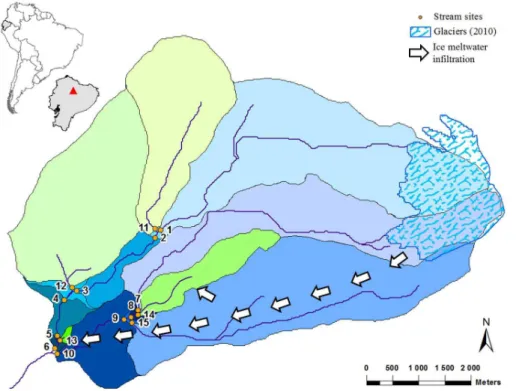
sites (no. 1–10; Fig. 1) were localized along two glacier-fed streams and five on their respective superficial tributaries (no. 11–15; Fig. 1). Among the studied tributaries, four stream sites (no. 11–14) were considered non-glacial as they had no glacier cover in their catchment (see Fig. 1) and did not present physico-chemical features generally

observed in glacier-fed streams (Brown et al., 2003), e.g. high turbidity (>30 NTU),

25

low conductivity (<10 µS cm−1) (see Table 1), and one site (no. 15) was partially fed

(7)

HESSD

10, 4369–4395, 2013

Title Page

Tables Figures

◭ ◮

Back Close

Full Screen / Esc

Discussion

P

a

per

|

Dis

cussion

P

a

per

|

Discussion

P

a

per

|

Discussio

n

P

a

per

|

a.s.l., one from the snout of the “Crespo” Glacier, which covered an area of about

1.82 km2at the time of the study in 2010; and the second from the snout of the Glacier

“14”, which covered an area of about 1.24 km2 (Rabatel et al., 2013). Stream sites

were all located between 4040 and 4200 m a.s.l., between 5.9 and 9.6 km away from

the glacier snouts. At the glacier snout, both streams had high turbidity (>285 NTU)

5

and low conductivity (<9 µS cm−1), which decreased and increased downstream,

re-spectively, in particular after confluences with tributaries (see Jacobsen et al., 2010; Kuhn et al., 2011 for details). Contrastingly, non-glacial tributaries presented high

con-ductivity (>60 µS cm−1) and low turbidity (<10 NTU, see Table 1 for details on the

physico-chemical characteristics of each stream site). 10

Field measurementsThe location of each stream site was measured using the UTM-WGS84 coordinates system with a GPS (Garmin Oregon 550, Garmin International Inc., Olathe, USA). In January 2010, 15 water pressure loggers were installed (Hobo water pressure loggers, Onset Computer Corp., USA) into the water at each stream site and recorded water pressure every 30 min over 10 months, i.e. from January to October 15

2010. Water pressure loggers were previously protected in plastic tubes placed verti-cally on the stream side where the sections were deep enough to avoid overflowing during the glacial flood and with homogeneous shapes among stream sites. One more logger was fixed on a rock at 4100 m a.s.l. to measure the atmospheric pressure every 30 min over the same 10 month period. Water level and height between the stream bot-20

tom and the Hobo sensor were measured twice, when the loggers were installed and removed.

3 Materials and methods

3.1 Wavelet transform analyses of water depth data

Our method proposes to use wavelet transform analyses on water depth time series to 25

(8)

HESSD

10, 4369–4395, 2013

Title Page

Tables Figures

◭ ◮

Back Close

Full Screen / Esc

Discussion

P

a

per

|

Dis

cussion

P

a

per

|

Discussion

P

a

per

|

Discussio

n

P

a

per

|

repeated cyclic fluctuations at the daily time-scale during the ablation period (Hannah et al., 1999, 2000), we aim to detect corresponding variations in daily water depth at 24 h scale and to determine the occurrence of these variations.

Previous works have reviewed in detail the concepts of wavelet analysis for different

applications (Daubechies, 1990; Torrence and Compo, 1998; Cazelles et al., 2008). 5

Here, we list some important concepts with special attention to properties used in this study. The wavelet transform analysis is a time-dependent spectral analysis that de-composes a data series in time-frequency space. The wavelet transforms therefore express a time series in a three-dimensional space: time (x), scale/frequency (y), and power (z). The power matches the magnitude of the variance in the series at a given 10

wavelet scale and time. Various types of wavelet functions (e.g. Morlet, Mexican hat, Paul) can be used for the signal transform, depending on the nature of the time se-ries and the objectives of the study. Here, we chose the Morlet wavelet, a nonorthog-onal, continuous, and complex wavelet function (with real and imaginary parts), be-cause it is particularly well adapted for hydrological time series analyses (Torrence 15

and Compo, 1998; Labat et al., 2000; Lafreneire and Sharp, 2003). Nonorthogonal continuous wavelet transforms are indeed more robust to noise than other decom-position schemes and are robust to variations in data length (Cazelles et al., 2008). Moreover complex wavelet functions are well suited for capturing oscillatory behavior whereas real wavelet functions do better to isolate peaks or discontinuities (Torrence 20

and Compo, 1998). Finally the Morlet wavelet function has a high resolution in fre-quency compared to other continuous wavelets (Cazelles et al., 2008), which was fun-damental in our method as we intended to detect the repeated water depth variations at the 24 h scale.

The continuous wavelet transform W_n(s) of a discrete time series x_n (n being the

25

time position) at scalesis defined as the convolution ofxnwith a scaled and translated

(9)

HESSD

10, 4369–4395, 2013

Title Page

Tables Figures

◭ ◮

Back Close

Full Screen / Esc

Discussion

P

a

per

|

Dis

cussion

P

a

per

|

Discussion

P

a

per

|

Discussio

n

P

a

per

|

W_n(s)= N−1 X

n′₌₀ x_n′ψ∗

_(n′₋_n)δt

s

(1)

whereN is the number of points in the time series, ψ∗(t) is the complex conjugate of

wavelet function (the Morlet wavelet in our case) at scalesand translated in time byn,

δtis the time step for the analysis (Torrence and Compo, 1998). The Morlet wavelet is

defined as: 5

ψ(t)=π−1/4ei6te−t2/2 (2)

wheretis a nondimensional “time” parameter.

In order to quantify the magnitude of the variance in the series at a given wavelet scale and location in time, we determined the local wavelet power spectrum (Torrence and Compo, 1998), defined as the squared absolute value of the wavelet transform 10

(|Wn(s)|2) and calculated as follows:

|Wn(s)|2=Wn(s)Wn∗(s) (3)

whereW_n∗(s) is the complex conjugate ofW_n(s).

To compare the spectral power of di_fferent stream sites, it was necessary to

deter-mine the global wavelet spectrum, which is the average of the local wavelet spectrum 15

at every scale over the whole time series (Torrence and Compo, 1998). The result is a graph of wavelet power versus scale, analogous to the Fourier power spectrum (see Cazelles et al., 2008), in which localization in time is lost. The global wavelet spectrum

|Wn(s)|2is defined as

|Wn(s)|2=

1 N

N−1 X

n=0

|Wn(s)|2 (4)

20

(10)

HESSD

10, 4369–4395, 2013

Title Page

Tables Figures

◭ ◮

Back Close

Full Screen / Esc

Discussion

P

a

per

|

Dis

cussion

P

a

per

|

Discussion

P

a

per

|

Discussio

n

P

a

per

|

3.2 Glacial signal determination

As glacier-fed streams are characterized by daily flood events, with discharge depend-ing on the rate of glacier melt (Milner et al., 2009), we determined the glacial influence on water depth time series as the occurrence of the daily glacial flood. As the global wavelet spectrum presents the average value of the wavelet power over the whole time 5

series at all scales, this measure provides an unbiased and consistent estimation of the true power spectrum of a time series (Percival, 1995). Therefore, we determined the glacial influence as the global wavelet power spectrum value at the 24 h scale, corrected by the corresponding significance level.

To use the wavelet power spectrum as a descriptor of glacial influence we needed to 10

test its significance in comparison to the expected spectrum of the background func-tion (Lafreneire and Sharp, 2003). Usually, the background (or noise) spectrum is either white noise (constant variance across all scales or frequencies) or red noise

(increas-ing variance with increas(increas-ing scale or decreas(increas-ing frequency, Schiff, 1992; Torrence and

Compo, 1998). When the wavelet power of the time series exceeds the power of the 15

background (at the chosen confidence level), the time series variance can be deemed significant (see Torrence and Compo, 1998; Lafreneire and Sharp, 2003 for background spectrum calculation details). Here, we chose the white-noise spectrum (at 95 % con-fidence level) as we were particularly interested in measuring the significance of the wavelet power spectrum at one specific scale, namely 24 h. The wavelet scale is often 20

expressed in terms of its equivalent Fourier period (Lafreneire and Sharp, 2003). How-ever, for the Morlet function the wavelet scale and Fourier period are almost equal

(pe-riod=1.03×scale), so the terms period and scale will hereafter be used

interchange-ably.

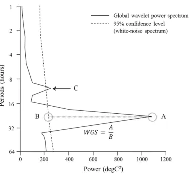
Based on the previous calculations, we defined the Wavelet Glacier Signal (WGS) 25

as the ratio between the global wavelet power spectrum value and its corresponding 95 % confidence level (white-noise spectrum) at the 24 h period (see Fig. 2: the glacier

(11)

HESSD

10, 4369–4395, 2013

Title Page

Tables Figures

◭ ◮

Back Close

Full Screen / Esc

Discussion

P

a

per

|

Dis

cussion

P

a

per

|

Discussion

P

a

per

|

Discussio

n

P

a

per

|

3.3 Application

To determine the WGS of water pressure time series obtained from the 15 stream sites we first transformed water pressure values into water depth values by subtract-ing the atmospheric variations from the water pressure data. Time series were cen-tered on their means and normalized by their standard deviations prior to wavelet 5

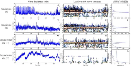
transform calculation to allow across-site and across-month comparison of our re-sults. We then used a code developed by C. Torrence and G. Compo (available at: http://paos.colorado.edu/research/wavelets) that we ran in MATLAB, version R2009a (The Mathworks Inc., Natick, MA, USA). This code allowed to produce three types of figures: (1) the water depth time series which presents the water depth variation 10

throughout the year; (2) the local wavelet spectrum which gives the magnitude (nor-malized by their standard deviations) and the occurrence of the variance in the series at a given wavelet scale and location time; and (3) the global wavelet spectrum which presents the average of the wavelet power and the white-noise spectrum over the whole time series, at all scales. For illustrative purposes, Fig. 3 presents in (A-L) the outputs 15

of our wavelet analyses for four stream sites (no. 1, 7, 12, and 14) with contrasting

time series patterns (resulting from different glacial influence): a glacier-fed stream site

without superficial tributaries (no. 7, Fig. 3a–c), a glacier-fed stream site with one non-glacial superficial tributary (no. 1, Fig. 3d–f), and two groundwater fed stream sites (no. 12 and 14, Fig. 3g–l). Then we determined the global wavelet spectrum value at 20

24 h period and its corresponding significance value to calculate the WGS for all stream sites.

3.4 Use and relevance of the WGS

3.4.1 WGS vs. percentage of the glacier cover in the stream catchment

The percentage of glacier cover in the catchment (hereafter GCC) is an index com-25

(12)

HESSD

10, 4369–4395, 2013

Title Page

Tables Figures

◭ ◮

Back Close

Full Screen / Esc

Discussion

P

a

per

|

Dis

cussion

P

a

per

|

Discussion

P

a

per

|

Discussio

n

P

a

per

|

2012). We therefore assessed the relevance of our WGS with regard to the percentage of GCC.

To measure the percentage of GCC, we first created the hydraulic channel network of our two study catchments using a 40 m resolution Digital Elevation Model (DEM) in SAGA GIS (System for Automated Geoscientific Analyses, version 2.0.8). The DEM 5

was created using 40 m resolution contour line from the Ecuadorian Military Geograph-ical Institute (available at: http://www.igm.gob.ec/site/index.php) in ARCGIS (10.0). We verified each created channel with our GPS point measurements and field observa-tions, and determined for each stream site the corresponding watershed using SAGA GIS (Olaya and Conrad, 2009).

10

Glacier outlines were first automatically extracted from LANDSAT satellite images

(30 m pixel size) using the common Normalized Difference Snow Index (NDSI). The

glacier outlines were then manually checked and adjusted by overlaying the glacier outline shapefile on the satellite images for which a spectral band combination associ-ating the shortwave infrared, the near infrared, and the green bands had been applied 15

(such a combination facilitates the distinction between snow, ice and rock, see Fig. 4 in Rabatel et al., 2012). We finally merged the glacier outlines and watershed contours shapefiles using ARCGIS 10.0. This enabled to compute the percentage of the glacier cover in the catchment basin of each stream site by dividing the glacier area by the total catchment basin area.

20

WGS data were plotted against the percentage of GCC and fitted with linear and curvilinear models in Table Curve 5.01 (Systat Software, Chicago, Illinois). Based on lowest Akaike Informatio Criteria values, the best model fitting the data was a linear model. The strength of the GCC vs. WGS correlation was measured using Spearman

correlation coefficients and associatedP values.

25

3.4.2 Comparison between 1 and 10 months water depth time series

(13)

HESSD

10, 4369–4395, 2013

Title Page

Tables Figures

◭ ◮

Back Close

Full Screen / Esc

Discussion

P

a

per

|

Dis

cussion

P

a

per

|

Discussion

P

a

per

|

Discussio

n

P

a

per

|

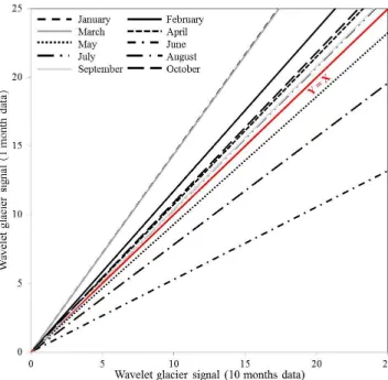
broken or stolen. It was therefore interesting to test whether WGS values calculated from short water depth time series (e.g. over one month) could be reliable surrogates of WGS values calculated over longer time periods (ten months in our case). To ad-dress this issue, we plotted for each stream site the WGS calculated from 10 months vs. the WGS calculated with one month data and then tested the significance of the 5

relationship using Spearman correlation coefficients. Between-month differences in the

slope of linear relationships were tested using an analysis of covariance (ANCOVA).

4 Results and discussion

4.1 Wavelet transform analyses

Most of the variance in the local and global wavelet spectra of sites 1 to 10 was concen-10

trated at the 24 h period (Fig. 3b, c, e and f). This diurnal wavelet power represented the daily glacial flood (Lafreneire and Sharp, 2003). At all sites along the two glacier-fed streams, the power of the local wavelet spectra at the 24 h period was statistically significant over the ten months (see Fig. 3b, e Table 1). Indeed glacial floods occur all year round in equatorial glacier-fed streams due to the absence of a perennial snow 15

cover outside the glaciers, daily diurnal melting, and nocturnal freezing (Favier et al., 2008; Jacobsen et al., 2010). However, the WGS decreased downstream in the two glacier-fed streams, from 19.9 (site 1) to 2.9 (site 6) and from 25.8 (site 7) to 8.0 (site 10, see Table 1). This decrease was more pronounced at sites located after a conflu-ence with a groundwater tributary (except for site 8, see discussion below), a pattern 20

already observed by Jacobsen and Dangles (2012) using their glacier index. Site 15, located on a tributary partially fed by glacial meltwater, also presented a significant (i.e.

>1) glaciar signal (WGS=2.2).

Although the diurnal wavelet power was significant in glacier-fed streams over the whole year, our data also showed that, at a few sites (e.g. site 7, Fig. 3a, b), gener-25

(14)

HESSD

10, 4369–4395, 2013

Title Page

Tables Figures

◭ ◮

Back Close

Full Screen / Esc

Discussion

P

a

per

|

Dis

cussion

P

a

per

|

Discussion

P

a

per

|

Discussio

n

P

a

per

|

between January and May while it was seldom significant after May. This phenomenon could be related to strongest ablation rates on the glaciers during this period of that year. Indeed, Rabatel et al. (2013) showed that during the period from January to April 2010 the Antisana glaciers experimented high ablation rates related to El Ni ˜no condi-tions (see Fig. 9 in Rabatel et al., 2013), which favored glacier melting. Contrastingly, 5

ablation is generally reduced under La Ni ˜na conditions (Francou et al., 2004).

As expected, sites 11 and 12, two non-glacial tributaries did not present any

sig-nificant power at the 24 h period (WGS<1, see Fig. 3k,l and Table 1), confirming the

relevance of WGS as a purely glacier signal (as all sites received a similar amount of precipitation, Villacis, 2008). Surprisingly, significant glacier signals were identified at 10

two supposedly non-glaciar sites (site 13 and 14, see Fig. 3h, i and Table 1). While these sites presented no glacier cover in their catchment and non-glaciar

characteris-tics (turbidity<9 NTU, conductivity>90 µS cm−1; see Fig. 1 and Table 1), our wavelet

analysis revealed a significant influence of the glacier all year round (see discussion below). The significant WGS at site 14 increased the WGS value at site 8 (located after 15

the confluence) when compared to upstream site (no. 7).

4.2 Comparison with the percentage of glacier cover in the catchment

We found a significant positive relationship between WGS and the percentage of

glacier cover in the catchment (Spearman rank test,r =0.761, F =19.13, p <0.001).

This strongly supports that our WGS could be used as a surrogate of the percentage of 20

glacier cover in the stream catchment. Figure 4 also shows that one WGS value (from sites no. 14) laid far above the correlation line. This site presented a highly significant WGS (20.4) while having no glacier cover in its catchment. This was also the case for

site no. 13 which presented a low but significant WGS value (WGS=1.5) although the

% GCC=0. These unexpected WGS values (black dots in Fig. 4) suggest infiltrations

25

(15)

HESSD

10, 4369–4395, 2013

Title Page

Tables Figures

◭ ◮

Back Close

Full Screen / Esc

Discussion

P

a

per

|

Dis

cussion

P

a

per

|

Discussion

P

a

per

|

Discussio

n

P

a

per

|

the whole watershed. The wavelet method allowed identifying such infiltrations using only data of water levels, making the WGS a powerful index to understand glacier in-fluence in watersheds with complex geological structure (which is more often the rule than the exception). Note that removing site 13 and 14 from the relationship between

WGS and % GCC increased markedly the correlation coe_fficient (r=0.94,F =98.92,

5

p <0.001). This confirmed that calculating the WGS may be a much better alternative to the % GCC as this latter does not permit to detect glacial meltwater reemergence, contrary to the WGS.

4.3 Relevance of WGS using short time series

For each month of the study period, we found significant relationships between WGS 10

calculated based on 30 day time series of water level and those based on 10 month time

series (Spearman rank test, 9.72< F <63.13, 0.48< r <0.87,p <0.01, see Fig. 5). In

other words, performing our wavelet methodology with data obtained over only one month was enough to detect the influence of glacier meltwater at each site of our study catchments, at a given period of the year. However, the slope of the 10 curves 15

presented in Fig. 5 significantly differed from each other in 84 % of cases (44 out of

56 potential pair comparisons, ANCOVA, df =24, F >4.10, p <0.05). Overall, WGS

from January to April, July, September and, October were higher than the “annual” WGS (1 : 1 line in Fig. 5) while those in May, June and, August were smaller than the “annual” WGS. This result suggests that any comparison of the glacial influence 20

among di_fferent sites should be realized with water level time series acquired over the

same time period. Indeed, the seasonality in weather conditions influences the relative contributions of water sources (e.g. ice, snow, rain, and groundwater, Ilg and Castella,

2006; Brown et al., 2009) with effects on discharge characteristics (Milner et al., 2009)

(16)

HESSD

10, 4369–4395, 2013

Title Page

Tables Figures

◭ ◮

Back Close

Full Screen / Esc

Discussion

P

a

per

|

Dis

cussion

P

a

per

|

Discussion

P

a

per

|

Discussio

n

P

a

per

|

5 Conclusions

Although wavelet analyses were used in climatology and hydrology since the end of the nineties (Smith et al., 1998), our study is one of the first to use this method to de-tect glacier influence in hydrosystems draining glacierized catchments. It is important to remember that wavelet analyses on water level time series do not allow quantify-5

ing the glacier contribution to the catchment runoff. While our WGS index determine

semi-quantitatively the influence of glaciers on glacier-fed hydrosystems (i.e. the WGS increases linearly with increasing glacier cover in the catchment), continuous stream

discharge time series would be necessary to quantify the relative contribution of diff

er-ent water sources at a given site. In this context, our method could be easily applicable 10

to discharge time series.

To conclude, we would like to highlight two key areas of novelty of our methodological approach. First, wavelet analyses present several advantages over methods that have been previously developed. Unlike many glacier indices (e.g. Milner and Petts, 1994; Brown et al., 2003, 2009; Ilg and Castella, 2006) our index does not include water 15

physico-chemical variables, which, in many cases, are not a reliable descriptors of glacial influence as they can be modified by many factors such as climate, bedrock substrates, and altitude (Nelson et al., 2011; Zhu et al., 2012). In particular, when glacial meltwater infiltrations occur, water chemistry is likely to be considerably modified during the underground flow routing, depending on the residence time underground, 20

the distance of the underground flow routing and the bedrock substrates (Hindshaw et al., 2011; Nelson et al., 2011). Importantly, our method allows detecting easily the influence of glacial meltwater reemergence on hydrosystems, a key improvement when compared to most existing methods.

Second, while we specifically focused on 10 month water level data in the tropical 25

(17)

HESSD

10, 4369–4395, 2013

Title Page

Tables Figures

◭ ◮

Back Close

Full Screen / Esc

Discussion

P

a

per

|

Dis

cussion

P

a

per

|

Discussion

P

a

per

|

Discussio

n

P

a

per

|

daily river discharge fluctuations (Milner at al., 2009). This pattern has been observed

in many di_fferent regions worldwide such as the tropical Andes (Rabatel et al., 2013),

the Himalayas (Sorg et al., 2012), the European Alps (Schutz et al., 2001), the North American Rockies (Lafreneire and Sharp, 2003), and the Arctic (Dahlke et al., 2012). Consequently, as daily floods always occur during the ablation season in any glacier-5

fed streams worldwide, our method is relevant not only in the tropics but also in tem-perate and arctic regions. Also, while we focused on daily fluctuations in our study, the WGS index could be easily calculated to detect glacier influence at higher time scale (seasonal, inter-annual), if longer time series are available. It could therefore

be a simple and cost-effective tool to track climate change impact on hydrosystems

10

draining glacierized catchments. Overall, our hope is that our WGS index may provide a testable and applicable methodological framework to better understand the complex interactions between glacier and glacier-fed hydrosystems in a warming world.

Acknowledgements. We thank Patricio Andino and Rodrigo Espinosa for technical support in

the field and Ma ¨elle Collet for the glacier outlines of Antisana. The funding by an Ecofondo 15

grant no. 034-ECO8-inv1 to O. D. and by a WWF-Novozymes grant 2008 to D. J. are greatly appreciated.

References

Baraer, M., Bryan, G., McKenzie, J. M., Condom, T., and Rathay, S.: Glacier recession and water resources in Peru’s Cordillera Blanca, J. Glaciol., 58, 134–150, 2012.

20

Barnett, T. P., Adam, J. C., and Lettenmaier, D. P.: Potential impacts of a warming climate on water availability in snow-dominated regions, Nature, 438, 303–309, 2005.

Bradley, R. S., Vuille, M., Diaz, H. F., and Vergara, W.: Threats to water supplies in the tropical Andes, Science, 312, 1755–1756, 2006.

Brown, L. E., Hannah, D. M., and Milner, A.: Alpine stream habitat classification: an alternative 25

(18)

HESSD

10, 4369–4395, 2013

Title Page

Tables Figures

◭ ◮

Back Close

Full Screen / Esc

Discussion

P

a

per

|

Dis

cussion

P

a

per

|

Discussion

P

a

per

|

Discussio

n

P

a

per

|

Brown, L. E., Hannah, D. M., and Milner, A. M.: ARISE: a classification tool for alpine river and stream ecosystems, Freshwater Biol., 54, 1357–1369, 2009.

Brown, L. E., Milner, A. M., and Hannah, D. M.: Predicting river ecosystem response to glacial meltwater dynamics: a case study of quantitative water sourcing and glaciality index ap-proaches, Aquat. Sci., 72, 325–334, 2010.

5

Cazelles, B., Chavez, M., Berteaux, D., M ´enard, F., Vik, J. O., Jenouvrier, S., and Stenseth, N. C.: Wavelet analysis of ecological time series, Oecologia, 156, 287–304, 2008. Condom, T., Escobar, M., Purkey, D., Pouget, J. C., Suarez, W., Ramos, C.,

Apaestegui, J.,Tacsi, A., and Gomez, J.: Simulating the implications of glaciers’ retreat for water management: a case study in the Rio Santa basin, Peru, Water Int., 37, 442–459, 10

2012.

Dahlke, H. E., Lyon, S. W., Jansson, P., Karlin, T., and Rosqvist, G.: Isotopic investigation of runo_ffgeneration in a glacierized catchment in northern Sweden, Hydrol. Process., online first, doi:10.1002/hyp.9668, 2012.

Daubechies, I.: The wavelet transform, time-frequency localization and signal analysis, IEEE T. 15

Inform. Theory, 36, 961–1005, 1990.

Favier, V., Coudrain, A., Cadier, E., Francou, B., Ayabaca, E., Maisincho, L., Praderio, E., Vil-lacis, M., and Wagnon, P.: Evidence of groundwater flow on Antizana ice-covered volcano, Ecuador/Mise en évidence d’ écoulements souterrains sur le volcan englac é Antizana, Equa-teur, Hydrolog. Sci. J., 53, 278–291, 2008.

20

Francou, B., Vuille, M., Favier, V., and C ´aceres, B.: New evidence for an ENSO impact on low-latitude glaciers: Antizana 15, Andes of Ecuador, 0 28′S, J. Geophys. Res, 109, D18106, doi:10.1029/2003JD004484, 2004.

F ¨ureder, L.: Life at the edge: habitat condition and bottom fauna of alpine running waters, Int. Rev. Hydrobiol., 92, 491–513, 2007.

25

Hannah, D. M., Gurnell, A. M., and McGregor, G. R.: A methodology for investigation of the seasonal evolution in proglacial hydrograph form, Hydrol. Process., 13, 2603–2621, 1999. Hannah, D. M., Gurnell, A. M., and Mcgregor, G. R.: Spatio–temporal variation in microclimate,

the surface energy balance and ablation over a cirque glacier, Int. J. Climatol., 20, 733–758, 2000.

30

(19)

HESSD

10, 4369–4395, 2013

Title Page

Tables Figures

◭ ◮

Back Close

Full Screen / Esc

Discussion

P

a

per

|

Dis

cussion

P

a

per

|

Discussion

P

a

per

|

Discussio

n

P

a

per

|

water chemistry in a glacial catchment (Damma Glacier, Switzerland), Chem. Geol., 285, 215–230, 2011.

Huss, M., Farinotti, D., Bauder, A., and Funk, M.: Modelling runofffrom highly glacierized alpine drainage basins in a changing climate, Hydrol. Process., 22, 3888–3902, 2008.

Ilg, C. and Castella, E.: Patterns of macroinvertebrate traits along three glacial stream continu-5

ums, Freshwater Biol., 51, 840–853, 2006.

Jacobsen, D. and Dangles, O.: Environmental harshness and global richness patterns in glacier-fed streams, Global Ecol. Biogeogr., 21, 647–656, 2012.

Jacobsen, D., Dangles, O., Andino, P., Espinosa, R., Hamerlik, L., and Cadier, E.: Longitudi-nal zonation of macroinvertebrates in an Ecuadorian glacier-fed stream: do tropical glacial 10

systems fit the temperate model?, Freshwater Biol., 55, 1234–1248, 2010.

Jacobsen, D., Milner, A. M., Brown, L. E., and Dangles, O.: Biodiversity under threat in glacier-fed river systems, Nature Climate Change, 2, 361–364, 2012.

Jiang, Y., Zhou, C. H., and Cheng, W. M.: Streamflow trends and hydrological response to climatic change in Tarim headwater basin, J. Geogr. Sci., 17, 51–61, 2007.

15

Kaser, G., Grosshauser, M., and Marzeion, B.: Contribution potential of glaciers to water avail-ability in different climate regimes, P. Natl. Acad. Sci. USA, 107, 20223–20227, 2010. Kuhn, J., Andino, P., Calvez, R., Espinosa, R., Hamerlik, L., Vie, S., Dangles, O., and

Jacob-sen, D.: Spatial variability in macroinvertebrate assemblages along and among neighbouring equatorial glacier fed streams, Freshwater Biol., 56, 2226–2244, 2011.

20

Labat, D.: Recent advances in wavelet analyses: Part I: A review of concepts, J. Hydrol., 314, 275–288, 2005.

Labat, D., Ababou, R., and Mangin, A.: Rainfall-runoffrelations for karstic springs. Part II: Con-tinuous wavelet and discrete orthogonal multiresolution, J. Hydrol., 238, 149–178, 2000. Lafreneire, M. and Sharp, M.: Wavelet analysis of inter-annual variability in the runoffregimes 25

of glacial and nival stream catchments, Bow Lake, Alberta, Hydrol. Process., 17, 1093–1118, 2003.

Lemke, P., Ren, J., Alley, R. B., Allison, I., Carrasco, J., Flato, G., Fujii, Y., Kaser, G., Mote, P., Thomas, R. H., and Zhang, T.: Observations: changes in snow, ice and frozen ground, in: Climate Change 2007: The Physical Science Basis, edited by: Solomon, S., Qin, D., Man-30

(20)

HESSD

10, 4369–4395, 2013

Title Page

Tables Figures

◭ ◮

Back Close

Full Screen / Esc

Discussion

P

a

per

|

Dis

cussion

P

a

per

|

Discussion

P

a

per

|

Discussio

n

P

a

per

|

Mathevet, T., Lepiller, M. l., and Mangin, A.: Application of time-series analyses to the hydro-logical functioning of an Alpine karstic system: the case of Bange-L’Eau-Morte, Hydrol. Earth Syst. Sci., 8, 1051–1064, doi:10.5194/hess-8-1051-2004, 2004.

Milner, A. M. and Petts, G. E.: Glacial rivers: physical habitat and ecology, Freshwater Biol., 32, 295–307, 1994.

5

Milner, A. M., Brown, L. E., and Hannah, D. M.: Hydroecological response of river systems to shrinking glaciers, Hydrol. Process., 23, 62–77, 2009.

Nelson, M. L., Rhoades, C. C., and Dwire, K. A.: Influence of bedrock geology on water chem-istry of slope wetlands and headwater streams in the southern Rocky Mountains, Wetlands, 31, 251–261, 2011.

10

Olaya, V. and Conrad, O.: Geomorphometry in SAGA, Dev. Soil Sci., 33, 293–308, 2009. Percival, D. P.: On estimation of the wavelet variance, Biometrika, 82, 619–631, 1995.

Rabatel, A., Bermejo, A., Loarte, E., Soruco, A., Gomez, J., Leonardini, G., Vincent, C., and Sicart, J. E.: Relationship between snowline altitude, equilibrium-line altitude and mass bal-ance on outer tropical glaciers: Glaciar Zongo – Bolivia, 16◦S and Glaciar Artesonraju – 15

Peru, 9◦S, J. Glaciol., 58, 1027–1036, 2012.

Rabatel, A., Francou, B., Soruco, A., Gomez, J., C áceres, B., Ceballos, J. L., Basantes, R., Vuille, M., Sicart, J.-E., Huggel, C., Scheel, M., Lejeune, Y., Arnaud, Y., Collet, M., Con-dom, T., Consoli, G., Favier, V., Jomelli, V., Galarraga, R., Ginot, P., Maisincho, L., Men-doza, J., M én égoz, M., Ramirez, E., Ribstein, P., Suarez, W., Villacis, M., and Wagnon, P.: 20

Current state of glaciers in the tropical Andes: a multi-century perspective on glacier evolu-tion and climate change, The Cryosphere, 7, 81–102, doi:10.5194/tc-7-81-2013, 2013. Rott, E., Cantonati, M., F ¨ureder, L., and Pfister, P.: Benthic algae in high altitude streams of the

Alps – a neglected component of the aquatic biota, Hydrobiologia, 562, 195–216, 2006. Sakakibara, D., Sugiyama, S., Sawagaki, T., Marinsek, S., and Skvarca, P.: Rapid retreat, ac-25

celeration and thinning of Glaciar Upsala, Southern Patagonia Icefield, initiated in 2008, Ann. Glaciol., 54, 131–138, 2013.

Schaefli, B., Maraun, D., and Holschneider, M.: What drives high flow events in the Swiss Alps? Recent developments in wavelet spectral analysis and their application to hydrology, Adv. Water Resour., 30, 2511–2525, 2007.

30

(21)

HESSD

10, 4369–4395, 2013

Title Page

Tables Figures

◭ ◮

Back Close

Full Screen / Esc

Discussion

P

a

per

|

Dis

cussion

P

a

per

|

Discussion

P

a

per

|

Discussio

n

P

a

per

|

Schutz, C., Wallinger, M., Burger, R., and Fureder, L.: Effects of snow cover on the benthic fauna in a glacier-fed stream, Freshwater Biol., 46, 1691–1704, 2001.

Smith, L. C., Turcotte, D. L., and Isacks, B. L.: Stream flow characterization and feature detec-tion using a discrete wavelet transform, Hydrol. Process., 12, 233–249, 1998.

Sorg, A., Bolch, T., Stoffel, M., Solomina, O., and Beniston, M.: Climate change impacts on 5

glaciers and runoffin Tien Shan (Central Asia), Nature Climate Change, 2, 725–731, 2012. Torrence, C. and Compo, G. P.: A practical guide to wavelet analysis, B. Am. Meteorol. Soc.,

79, 61–78, 1998.

Villacis, M.: Ressources en eau glaciaire dans les Andes d’Equateur en relation avec les vari-ations du climat: le cas du volcan Antisana, Ph.D thesis, Universit ´e Montpellier II, France, 10

250 pp., 2008.

(22)

HESSD

10, 4369–4395, 2013

Title Page

Tables Figures

◭ ◮

Back Close

Full Screen / Esc

Discussion

P

a

per

|

Dis

cussion

P

a

per

|

Discussion

P

a

per

|

Discussio

n

P

a

per

|

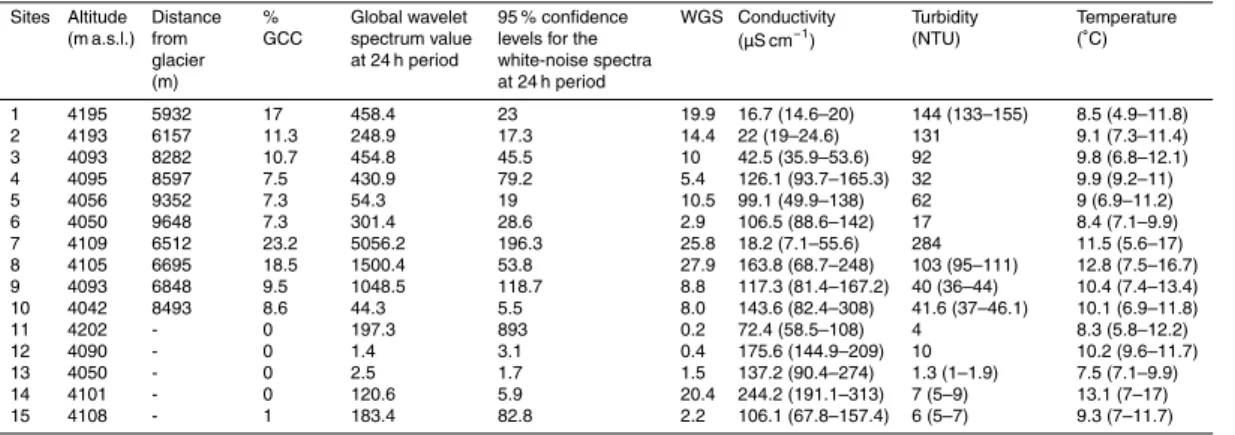
Table 1. Physico-chemical attributes of the study stream sites (see location of the sites on

Fig. 1). Conductivity, turbidity, and temperature are means with min–max values given in brack-ets (n=2 to 10 for conductivity and temperatures;n=1 to 3 for turbidity). Stream sites no. 11 to 15 have no visible connection to the glacier. GCC=glacier cover in the catchment. WGS

=wavelet glacier signal (see Methods). WGS is significant for values above 1 (see Methods). For details on the calculation of global wavelet spectrum and 95 % intervals see the text in the Methods and Fig. 2.

Sites Altitude (m a.s.l.)

Distance from glacier (m)

% GCC

Global wavelet spectrum value at 24 h period

95 % confidence levels for the white-noise spectra at 24 h period

WGS Conductivity

(µS cm−1₎ Turbidity_(NTU) Temperature₍◦_C)

1 4195 5932 17 458.4 23 19.9 16.7 (14.6–20) 144 (133–155) 8.5 (4.9–11.8) 2 4193 6157 11.3 248.9 17.3 14.4 22 (19–24.6) 131 9.1 (7.3–11.4) 3 4093 8282 10.7 454.8 45.5 10 42.5 (35.9–53.6) 92 9.8 (6.8–12.1) 4 4095 8597 7.5 430.9 79.2 5.4 126.1 (93.7–165.3) 32 9.9 (9.2–11)

5 4056 9352 7.3 54.3 19 10.5 99.1 (49.9–138) 62 9 (6.9–11.2)

6 4050 9648 7.3 301.4 28.6 2.9 106.5 (88.6–142) 17 8.4 (7.1–9.9) 7 4109 6512 23.2 5056.2 196.3 25.8 18.2 (7.1–55.6) 284 11.5 (5.6–17) 8 4105 6695 18.5 1500.4 53.8 27.9 163.8 (68.7–248) 103 (95–111) 12.8 (7.5–16.7) 9 4093 6848 9.5 1048.5 118.7 8.8 117.3 (81.4–167.2) 40 (36–44) 10.4 (7.4–13.4) 10 4042 8493 8.6 44.3 5.5 8.0 143.6 (82.4–308) 41.6 (37–46.1) 10.1 (6.9–11.8)

11 4202 - 0 197.3 893 0.2 72.4 (58.5–108) 4 8.3 (5.8–12.2)

12 4090 - 0 1.4 3.1 0.4 175.6 (144.9–209) 10 10.2 (9.6–11.7)

(23)

HESSD

10, 4369–4395, 2013

Title Page

Tables Figures

◭ ◮

Back Close

Full Screen / Esc

Discussion

P

a

per

|

Dis

cussion

P

a

per

|

Discussion

P

a

per

|

Discussio

n

P

a

per

|

Fig. 1.Study area at the Antisana Volcano, Ecuador. Stream sites are represented by orange

(24)

HESSD

10, 4369–4395, 2013

Title Page

Tables Figures

◭ ◮

Back Close

Full Screen / Esc

Discussion

P

a

per

|

Dis

cussion

P

a

per

|

Discussion

P

a

per

|

Discussio

n

P

a

per

|

Fig. 2.Theoretical illustration of the wavelet glacier signal (WGS) calculation. Black line

(25)

HESSD

10, 4369–4395, 2013

Title Page

Tables Figures

◭ ◮

Back Close

Full Screen / Esc

Discussion

P

a

per

|

Dis

cussion

P

a

per

|

Discussion

P

a

per

|

Discussio

n

P

a

per

|

Fig. 3.Wavelet analysis outputs at four stream sites (7, 1, 14, and 12) with contrasting glacial

(26)

HESSD

10, 4369–4395, 2013

Title Page

Tables Figures

◭ ◮

Back Close

Full Screen / Esc

Discussion

P

a

per

|

Dis

cussion

P

a

per

|

Discussion

P

a

per

|

Discussio

n

P

a

per

|

Fig. 4.Scatter plot of the wavelet glacier signal (WGS) vs. the percentage of glacier cover in the

(27)

HESSD

10, 4369–4395, 2013

Title Page

Tables Figures

◭ ◮

Back Close

Full Screen / Esc

Discussion

P

a

per

|

Dis

cussion

P

a

per

|

Discussion

P

a

per

|

Discussio

n

P

a

per

|

Fig. 5.Scatter plot of “monthly” wavelet glacier signal vs. “annual” wavelet glacier signal for