Simulation Model of Hydro Power Plant Using Matlab/Simulink

Simulation Model of Hydro Power Plant Using Matlab/Simulink

Mousa Sattouf*

*(Department of Electrical Power Engineering, Brno University of Technology, Czech Republic)

ABSTRACT

Hydropower has now become the best source of electricity on earth. It is produced due to the energy provided by moving or falling water. History proves that the cost of this electricity remains constant over the year. Because of the many advantages, most of the countries now have hydropower as the source of major electricity producer. The most important advantage of hydropower is that t is green energy, which mean that no air or water pollutants are produced, also no greenhouse gases like carbon dioxide are produced which makes this source of energy environment-friendly. It prevents us from the danger of global warming. This paper describes a generalized model which can be used to simulate a hydro power plant using MATLAB/SIMULINK. The plant consists of hydro turbine connected to synchronous generator, which is connected to public grid. Simulation of hydro turbine and synchronous generator can be done using various simulation tools, In this work, SIMULINK/MATLAB is favored over other tools in modeling the dynamics of a hydro turbine and synchronous machine. The SIMULINK program in MATLAB is used to obtain a schematic model of the hydro plant by means of basic function blocks. This approach is pedagogically better than using a compilation of program code as in other software programs .The library of SIMULINK software programs includes function blocks which can be linked and edited to model. The main objectives of this model are aimed to achieve some operating modes of the hydro plant and some operating tests.

Keywords

–

I.

INTRODUCTION

This paper describes the dynamic model of the two main components of hydro power plants, the synchronous generator and the hydro turbine governor.

The synchronous machine’s dynamic model

equations in the Laplace domain can be created by connecting appropriate function blocks. In order to simulate the detailed transient analysis of the synchronous machine, addition of new sub-models is needed to model the operation of various control functions. These sub-models are used in the calculation of various values related to the synchronous machine such as the steady state, exciter loop, turbine governor model and the currents.

Detailed mathematical representation of the hydraulic turbine-penstock also presented in this paper.. The dynamic performance of the hydraulic system is studied using time domain and frequency domain methods. The introduced mathematical representation of a hydraulic system is including both turbine-penstock and the governing system. The primary source for the electrical power provided by utilities is the kinetic energy of water which is converted into mechanical energy by the prime movers. The electrical energy to be supplied to the end users is then transformed from mechanical energy by the synchronous generators. The speed governing system adjusts the generator

speed based on the input signals of the deviations of both system frequency and interchanged power with respect to the reference settings. This is to ensure that the generator operates at or near nominal speed at all times.

Simulation of the three-phase synchronous machine and hydro turbines is well documented in the literature and a digital computer solution can be performed using various methods. This paper discusses the use of SIMULINK software of MATLAB, in the dynamic modeling of the hydro plant components. The main advantage of SIMULINK over other programming software is that, instead of compilation of program code, the simulation model is built up systematically by means of basic function blocks. To be able to model the dynamics of the hydro power plant, dynamic behavior or differential equations of the synchronous machine as well as hydro turbine need to be considered.

II.

S

M

M

This section describes a generalized model which can be used to simulate a three-phase. P-pole, symmetrical synchronous machine in rotating qd reference frame.

2.1THE D–QMODEL OF SYNCHRONOUS MACHINE

A model of synchronous generator in q-d rotating reference frame was developed. The main

aim of the d–q model is to eliminate the dependence of inductances on rotor position. To do so, the system of coordinates should be attached to the machine part that has magnetic saliency- the rotor for synchronous generators.[1]

The d–q model should express both stator and rotor equations in rotor coordinates, aligned to rotor d and q axes because, at least in the absence of magnetic saturation, there is no coupling between the two axes. The rotor windings f, D, Q are already aligned along d and q axes.

It is only the stator voltages, VA, VB, VC,

currents IA, IB, IC, and flux linkages ΨA, ΨB, ΨC

that have to be transformed to rotor orthogonal coordinates. The transformation of coordinates ABC to d–q-0, known also as the Park transform, valid for voltages, currents, and flux linkages as well, it is as follows:

(1)

Then will be:

(2)

(3)

(4)

The phase quantites, as phase currents IA, IB, IC are recovered from Id, Iq, I0 by:[2] (5)

the q and d axis for The d–q model of synchronous machine are shown in Fig. 1[1] Fig.1 d and q axises of synchronous machine 2.2VOLTAGE EQUATIONS OF THE SYNCHRONOUS MACHINE We shall next show the Voltage Equations of a threephase, P-pole, symmetrical synchronous machine in the rotating qd reference frame. Figure 2 showes the equivelant circuit of synchronous machine in qd axises. The following sets of equations (6),(7),(8),(9),(10),(11),(12),(13),(14) describe the general model of synchronous generator:[3] (6) (7)

(8)

(9)

(10)

(11)

(12)

(14)

The resistances and inductances are illustrated in the q and d equivalent circuits of synchronous machine. in Fig.2.

Fig.2 The q and d equivalent circuits of synchronous machine

Where:

, flux linkages among d and q axes.

, mutual flux linkages among d and q axes , d and q currents.

, flux linkages of damper coils among d and q axes

, currents of damper coils among a and q axes

2.3TORQUE EQUATION

The equation of motion of the rotor is obtained by equating the inertia torque to the accelerating torque, that is:

(15)

Where J is the inertia torque of the rotor, is the electromagnetic torque, is the externally-applied torque in the direction of the rotor speed and

is the damping torque in the direction opposite to rotation. The value of will be negative for the motoring condition.[1]

The electromagnetic torque is given by (16) as:

(16)

Where P is poles number.

III.

H

T

M

Power system performance is a acted by dynamic characteristics of hydraulic governor-turbines during and following any disturbance, such as occurrence of a fault, loss of a transmission line or a rapid change of load. Accurate modeling of hydraulic governor-turbines is essential to characterize and diagnose the system response during an emergency. Simple hydraulic systems governed by proportional-integral-derivative and proportional-integral controllers are modeled. This model examines their transient responses to disturbances through simulation in Matlab/Simulink.[4]

Fig.3 block diagram of the hydraulic governor-turbine system

Fig.3 shows a block diagram of the hydraulic governor-turbine system connected to a power system network. The primary source for the electrical power provided by utilities is the kinetic energy of water which is converted into mechanical energy by the prime movers. The electrical energy to be supplied to the end users is then transformed from mechanical energy by the synchronous generators. The speed governing system adjusts the generator speed based on the input signals of the deviations of both system frequency and interchanged power with respect to the reference settings. This is to ensure that the generator operates at or near nominal speed at all times. The hydraulic unit characteristic of a single penstock is:

(17)

(18)

Where q is turbine flow, is initial steady-state head, h is hydraulic head at gate, is head losses due to friction in the conduit, is gravity acceleration, A ispenstock cross section area, L is conduit length, is ideal gate opening based on the change from the no load to full load being equal to 1 per unit.[5]

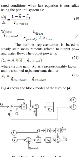
rated conditions when last equation is normalized using the per unit system as:

(19)

Where:

(20)

The turbine representation is based on steady state measurements related to output power and water flow. The output power is:

(21)

where turbine gain is a proportionality factor and is assumed to be constant, that is:

(22)

Fig.4 shows the block model of the turbine.[4]

Fig.4 Hydraulic turbine block diagram

IV.

E

S

M

An excitation system model is described. Type DC excitation systems without the exciter's saturation, which utilize a direct current generator with a comutmator as the source of excitation system power.

This model, described by the block diagram of Fig 4, is used to represent field controlled dc commutator exciters with continuously acting voltage regulators.

Fig. 4 Excitation system block diagram

The principal input to this model is the output, , from the terminal voltage transducer and load compensator model. At the summing junction, terminal voltage transducer output, , is subtracted from the set point reference, . The stabilizing feedback, , is subtracted, and the power system stabilizing signal, , is added to produce an error voltage. In the steady-state, these last two signals are zero, leaving only the terminal voltage error signal. The resulting signal is ampliÞed in the regulator. The major time constant, , and gain, , associated with the voltage regulator, These voltage regulators utilize power sources that are essentially unaffected by brief transients on the synchronous machine or auxiliaries buses. The time constants, and may be used to model equivalent time constants inherent in the voltage regulator; but these time constants are frequently small enough to be neglected, and provision should be made for zero input data.[6]

The voltage regulator output, , is used to control the exciter, The exciter is represented by the following transfer function between the exciter voltage and the regulator's output :[6]

(23)

A signal derived from field voltage is normally used to provide excitation system stabilization, , via the rate feedback with gain, , and time constant, .

V.

S

R

Fig.5 Synchronous machine model

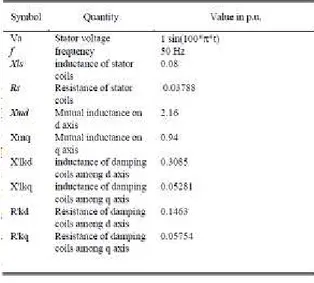
Using this model with hydraulic turbine model and excitation system model, which are presented previously in this paper, using those models we can easily simulate hydro power plant. Table 1 shows the synchronous machine parameters used in simulation.

Table 1 Synchronous machine parameters

The headings and subheadings, starting with "1. Introduction", appear in upper and lower case letters and should be set in bold and aligned flush left. All headings from the Introduction to Acknowledgements are numbered sequentially using 1, 2, 3, etc. Subheadings are numbered 1.1, 1.2, etc. If a subsection must be further divided, the numbers 1.1.1, 1.1.2, etc.

The font size for heading is 11 points bold face

Table 2 shows turbine parameters, while Table 2 shows excitation system parameters.

Table 2 hydro turbine model parameters

Table 3 excitation system parameters

Fig.6 per unit stator currents Iabc, stator voltage Va, excitation voltage Vf

Fig.7 per unit speed, output mechanical power of the turbine Pm

Fig.8 and Fig.9 show the system response for three phase fault at the generator terminals in time 2 to 2.2, where Fig.8 shows stator volages and currents before, during and after the fault, while Fig.9 shows the mechanical power and speed changes becuase of the fualt.

Fig.8 stator voltage Va, stator currents Iabc

Fig.9 Output mechanical power of the turbine Pm, Speed per unit.

VI.

C

SIMULINK is a powerful software package for the study of dynamic and nonlinear systems. Using SIMULINK, the simulation model can be built up systematically starting from simple sub-models. The hydro power plant model developed may be used alone, as in the direct-on-line starting example presented, or it can be incorporated in an advanced drive system. Several tests and operating conditions can be applied on the model. In this paper a three phase fault case was shown, many other faults or operating conditions as over load conditions can be applied and examined by this model. The author believe that SIMULINK will soon become an indispensable tool for the teaching and research of electrical machine drives.

REFERENCES

[1] C.M. Ong, Dynamic Simulation of Electric

Machinery Using Matlab/Simulink (A

[2] A.A. ANSARI, D.M. DESHPANDE, Mathematical Model of Asynchronous Machine in MATLAB Simulink,

International Journal of Engineering

Science and Technology, 2(5), 2010,

1260-1267.

[3] T. Kano, T. Ara, and T. Matsumura, A method for calculating equivalent circuit constants of a synchronous generator with damper using a dc decay test with open and shorted field windings, Proceedings of the 2008 International Conf. on Electrical

Machines, IEEE, 2008,

978-1-4244-1736-0.

[4] Y. C. choo, K. M. Muttaqi, and M. Negnevitsky, Modeling of hydraulic povernor-turbine for control stabilization,

Anzima Journal, 49(EMAC2007), 2008,

681-698.

[5] W.li, L. Vanfretti, and Y. Chompoobutrgool, Development and implementation of hydro turbine and governor models in a free and open source software package, Simulation Modeling Practice and Theory, 24, 2012, 84-102. [6] IEEE Standards Board, IEEE

Recommended Practice for Excitation System Models for Power System Stability Studies, IEEE Std 421.5-1992.

BIBLOGRAPHY