www.hydrol-earth-syst-sci.net/18/3095/2014/ doi:10.5194/hess-18-3095-2014
© Author(s) 2014. CC Attribution 3.0 License.
Using similarity of soil texture and hydroclimate to enhance soil
moisture estimation
E. J. Coopersmith1, B. S. Minsker1, and M. Sivapalan1,2
1Department of Civil & Environmental Engineering, University of Illinois at Urbana-Champaign, Urbana, IL 61801, USA 2Department of Geography and Geographic Information Science, University of Illinois at Urbana-Champaign, Urbana, IL 61801, USA
Correspondence to:E. J. Coopersmith ([email protected])
Received: 17 January 2014 – Published in Hydrol. Earth Syst. Sci. Discuss.: 25 February 2014 Revised: 7 July 2014 – Accepted: 12 July 2014 – Published: 20 August 2014
Abstract. Estimating soil moisture typically involves cali-brating models to sparse networks of in situ sensors, which introduces considerable error in locations where sensors are not available. We address this issue by calibrating parame-ters of a parsimonious soil moisture model, which requires only antecedent precipitation information, at gauged tions and then extrapolating these values to ungauged loca-tions via a hydroclimatic classification system. Fifteen sites within the Soil Climate Analysis Network (SCAN) contain-ing multiyear time series data for precipitation and soil mois-ture are used to calibrate the model. By calibrating at 1 of these 15 sites and validating at another, we observe that the best results are obtained where calibration and valida-tion occur within the same hydroclimatic class. Addivalida-tionally, soil texture data are tested for their importance in improv-ing predictions between calibration and validation sites. Re-sults have the largest errors when calibration–validation pairs differ hydroclimatically and edaphically, improve when one of these two characteristics are aligned, and are strongest when the calibration and validation sites are hydroclimati-cally and edaphihydroclimati-cally similar. These findings indicate con-siderable promise for improving soil moisture estimation in ungauged locations by considering these similarities.
1 Introduction
Soil moisture estimates are needed routinely for many prac-tical applications, such as irrigation scheduling and opera-tion of farm machinery. They are typically produced either through remote sensing or sparse networks of in situ
sen-sors. Although recent remote sensing studies have confirmed that such measurements approximate in situ sensor networks (Jackson et al., 2012), satellite-based sensors provide mea-surements at a spatial resolution of several kilometers – too large for daily agricultural decision making. On the other hand, in situ sensor networks produce values that are difficult to generalize to locations with no proximal sensors. Under these circumstances, dynamic soil moisture evolution models are typically used for soil moisture estimation at the desired location, using information from the nearest available sen-sors. This method of soil moisture estimation immediately raises the issue regarding the type of model that is most ap-propriate for such an application. One could think of several different types of models that may be suitable.
can be addressed using a soil water balance model, this type of model must be recalibrated frequently, which most soil moisture models are not, as its errors are cumulative (Jones, 2004).
The second group of models adopts a process-based ap-proach, estimating soil moisture from surface radiation and precipitation (Capehart and Carlson, 1994). These process-based models are typically forced by evapotranspiration de-mand and precipitation at their upper boundary and, if ap-plicable, by groundwater at their lower boundary. More so-phisticated models of this type, such as HYDRUS (Simunek et al., 1998), attempt to improve predictions via detailed knowledge of hydraulic soil parameters, information regard-ing root structures, soil temperature readregard-ings, and detailed at-mospheric/meteorological information, which are not widely available, especially for routine applications envisaged here. The third group of models is agriculturally focused, build-ing model projections outward from existbuild-ing instrumenta-tion and addiinstrumenta-tional measurements. Gamache et al. (2009) de-veloped a soil drying model for which cone penetrometers and soil moisture sensors are required. At most remote sites, these data sources are not currently accessible. Another simi-lar approach employs specific soil type information (theoret-ically, publicly available data), but ultimately requires prox-imal sensors to provide the needed soil moisture estimates (Chico-Santamaria et al., 2009).
Pan et al. (2003) and Pan (2012) addressed many of the shortcomings of the existing modeling approaches reviewed above by developing what they called a “diagnostic soil moisture equation” (i.e., model) in the form of a partial dif-ferential equation representing the lumped water balance of a vertical soil column, and representing the soil moisture at any moment in time as a function of the sum of a temporally de-caying sequence of observed past rainfall events. The model has the advantage that initial soil moisture conditions are not required (only antecedent precipitation data), nor must the model be recalibrated periodically. However, this approach does require a soil moisture sensor at the relevant location for initial calibration of the model’s parameters. This method has the disadvantage that the presence of soil heterogeneity could necessitate a large number of sensors to account for the spatial variation of soil moisture (Pan and Peters-Lidard, 2008). Furthermore, decision support often requires estima-tion at locaestima-tions lacking sensors.
The aim of this paper is to present and test an approach that can help overcome the issues of calibration at ungauged locations associated with the Pan et al. (2003) soil mois-ture estimation model. The proposed solution involves cal-ibrating the Pan (2012) diagnostic soil moisture equation (model) at gauged sites and then extrapolating the calibrated model to ungauged sites by invoking similarity. Similarity here is defined on the basis of hydroclimatic characteristics, using a classification system developed by Coopersmith et al. (2012), as well as edaphic (soil) properties. The proposed new scheme maintains the advantage of the parsimonious
soil moisture model of Pan et al. (2003) in that it does not re-quire specification of initial soil moisture condition, and also there is no need to recalibrate periodically. The model’s sim-plicity also permits implementation of the model in a manner that can easily be refit with new parameters, where necessary. Section 2 provides more details on the approach.
To calibrate and validate the model, data from the US Department of Agriculture’s (USDA) Soil Climate Analysis Network (SCAN) were used (Schaefer et al., 2007). This na-tional array of soil moisture sensors (with co-located precipi-tation sensors) delivers hourly data at a variety of publicly ac-cessible sites throughout the United States. Fifteen sensor lo-cations with numerous years of high-quality, minimally inter-rupted data were selected for further analysis. These sites dis-play considerable hydrologic diversity, which aids in demon-strating that the nationwide application of the proposed soil moisture model using precipitation data represents a feasi-ble goal. With respect to agricultural decision support, for energy-limited sites, the value of hourly soil moisture es-timates is found in the determination of whether or not a field is trafficable – whether heavy equipment will damage fields or become mired. With respect to water-limited sites, the value of soil moisture estimates is found in devising op-timal irrigation strategies that utilize limited water resources most efficiently. Of the 15 SCAN sites examined, the 3 sites in New Mexico, the site in Colorado, the site in Nebraska, the site in Wyoming, and the 2 in Iowa are all water-limited (8 in total). The remaining sites (7 in total) – located in Pennsylva-nia (2), Arkansas, Georgia, South Carolina, North Carolina, and Virginia – are all energy-limited. Results of the analysis are given in Sect. 3, followed by discussion in Sect. 4 to sug-gest further improvements, and conclusions are presented in Sect. 5.
2 Methodology
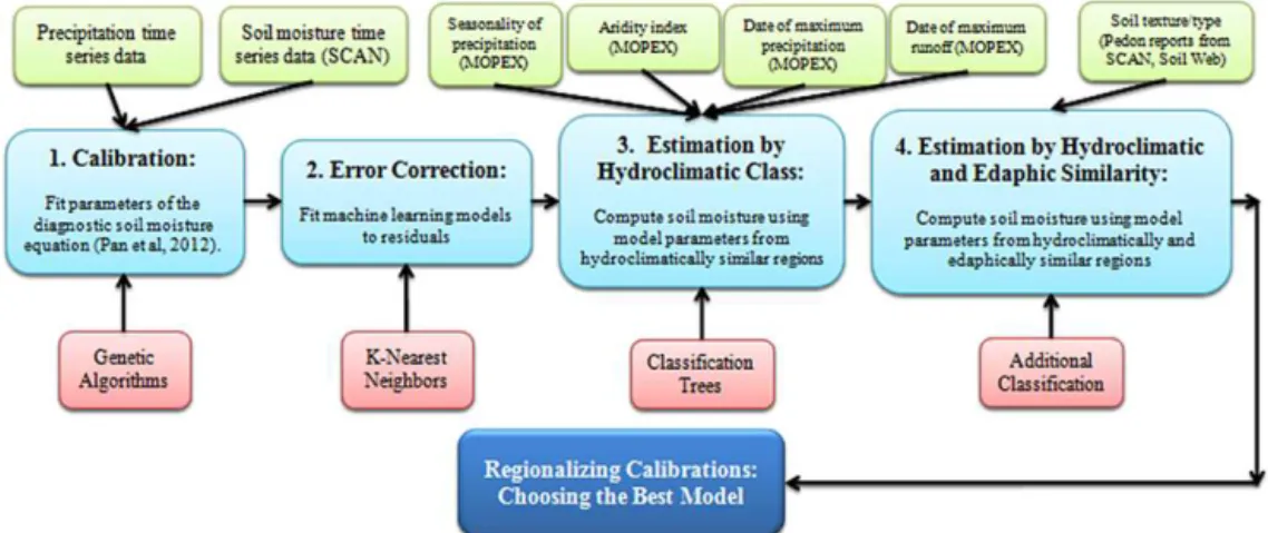
Figure 1.Methodological flow chart.
2.1 Step 1: calibration using a two-layer genetic algorithm
Unlike the original diagnostic soil moisture calibrations, the ultimate objective of this work is to enable agricultural deci-sion support in near-real time. To this end, the daily model from Pan (2012) is first modified to yield an hourly model within the same framework. Genetic algorithms (GAs) are then deployed to calibrate the model, enabling more effi-cient exploration of the parameter search space than the tra-ditional Monte Carlo search, which was the approach taken by Pan (2012).
GAs, a subset of evolutionary algorithms, were originally developed by Barricelli (1963) and have become increas-ingly common in environmental and water resources appli-cations, including the calibration of hydrologic model pa-rameters (e.g., Cheng et al., 2006; Singh and Minsker, 2008; Zhang et al., 2009).
In this work, a simple genetic algorithm uses the oper-ations of selection, crossover, and mutation (for reference, see Goldberg, 1989) to search for parameters that minimize prediction errors from the diagnostic soil moisture equation (Pan, 2012):
θest=θre+(φe−θre) 1−e−c4β. (1)
Here θestrepresents the best estimate of soil moisture dur-ing a given hour.θredenotes residual soil moisture, the min-imum quantity of moisture that is present regardless of the length of time without precipitation.φe, the soil’s porosity, signifies the maximum possible soil moisture value, at which point the soil becomes saturated. Finally, c4is a parameter related to conductivity and drainage properties, essentially defining the rate at which soil can dry. Ifc4assumes a value of zero, the soil is permanently at its residual soil moisture value,θre– a soil that dries infinitely rapidly. Conversely, as
c4becomes large, the soil will permanently assume the value of its porosity,φe– a soil that dries infinitely slowly. Theβ
term in Eq. (1) is calculated in Eq. (2) below:
β=
i=n−1
X
i=2
Pi ηi
1−e−ηiz
e
−
j=i−1
P
j=1
ηj
z
+
P1 η1
1−e−ηz1
. (2)
Here,Pidenotes the quantity of rainfall during houri(day in
the original presentation in Pan et al., 2003). The soil depth at which an estimation occurs is given byz. This convolution summation has a temporal window ofnhours for consider-ing past precipitation. For instance, today’s soil moisture is strongly influenced by yesterday’s rainfall, influenced to a lesser degree by last week’s rainfall, and not influenced at all by rainfall from 10 years prior. Given the general limitation of our data sets and the fact that shallow-depth soil moisture is most relevant to decision support, all of our analyses occur with measurements of 2 in. (∼5 cm) depth.
To choose the appropriate value forn, the value ofβ is calculated at each hour throughout the data set – settingn
to a very large value (2000 h, denoted byM)initially. Next this “beta series” (wheren=M)is correlated with a separate beta series, calculated wheren≪M. If the correlation coef-ficient between these two time series approaches unity, then the smaller value ofnis selected. Otherwise,nis increased incrementally until the correlation between then≪Mbeta series and then=Mbeta series approaches unity.
Finally, the estimated soil water loss at houri, e.g., due to evapotranspiration or deep drainage, is expressed by the termηi. As this algorithm does not presume any more
in Eq. (3):
η=αsin(i−δ)+γ . (3)
Here, αrepresents the sinusoid’s amplitude, γ denotes the vertical shift, andδsignifies the necessary phase shift. These three parameters are fitted via the genetic algorithm such that the correlation between the beta series (using the eta series implied byα,γ, andδ)and the observed soil moisture series
(θobs)is maximized. Once values for the eta series are es-tablished, the remaining three parameters of Eq. (1) (θre,φe, andc4)are then fitted by a second application of the genetic algorithm, this time minimizing the sum of squared errors between the estimated soil moisture series(θest)and the ob-served values(θobs).
2.2 Step 2: error correction using thek -nearest-neighbor machine learning algorithm
After the parameters of the diagnostic soil moisture equation (Eq. 1) have been calibrated, the hourly precipitation time se-ries is used to generate a soil moisture time sese-ries during the growing season months of interest. Discrepancies between the observed soil moisture values (θobs)and the estimated values(θest)are computed as shown in Eq. (4):
θobs=θest+ε, (4)
whereεrepresents the error associated with any hour’s soil moisture estimate.
To correct biases in these errors, the k-nearest-neighbor algorithm (KNN; Fix and Hodges, 1951) is employed to predict ε using the characteristics from the training data. More specifically, the data are searched for the most simi-lar matches in terms of time of day, day of year,θest,β(n), andβ (M)−β(n). For example, if the model returns a pre-diction ofθest=0.35 at 14:00 LT during July when rainfall has been heavy recently but drier over a longer period, KNN will search the training set for other estimates near 0.35 made on mid-summer afternoons where a similar recent rainfall pattern has been observed. Next, the algorithm averages the value of the error, ε, associated with those types of condi-tions, producing an estimated error,εest. Each validation es-timate is then adjusted to beθest+εest. This technique allows consistent model biases, such as underestimating wetter days and overestimating drier days, to be corrected.
This error correction model also accounts for diurnal soil moisture variations that were not considered in developing the diagnostic soil equation, which was designed to deliver daily soil moisture estimates. Consider a soil moisture esti-mate at 16:00, after soil has had a full day of sunlight (the-oretically) to dry. As the diagnostic soil moisture equation only considers drainage and evapotranspiration losses on a daily basis, θest will be larger than θobs. Yet, because this type of mistake presumably occurred frequently throughout the training data, the algorithm will locate other 16:00 esti-mates, each of which will be biased in the same direction,
and our final soil moisture estimates will take this bias into account, improving the results as shown subsequently.
To assess the performance of the soil moisture models with and without machine learning, anR2 value as defined in Eq. (5) is used, as this value represents the proportion of variance in soil moisture explained by the developed model:
R2=1−SSR
SST, (5)
where SSR denotes the sum of squared residuals and the SST term signifies the total sum of squares, i.e., the sample’s vari-ance.
2.3 Step 3: estimation by hydroclimatic similarity
This step tests the hypothesis that the classification system by Coopersmith et al. (2012) can be used to generalize the cal-ibrated parameters for the diagnostic soil moisture equation using hydroclimatic similarity. If two locations are assigned the same hydroclimatic classification, then the calibrated pa-rameters from one SCAN sensor within that class will be as-sumed to perform well at another.
This hypothesis was tested at 15 SCAN sensors for which soil moisture and precipitation data are available hourly for a period of several years. These sensors are located in diverse geographic locations and hydroclimatic classes in Iowa, North Carolina, Pennsylvania, New Mexico, Arkansas, Georgia, Virginia, South Carolina, Nebraska, Colorado, and Wyoming. The data at each of these locations were divided into training/validation sets, and parameters were calibrated using training data only. Next, these parameters were em-ployed on the validation sets at the locations for which they were calibrated. The subsequent R2 values (proportion of variance in soil moisture explained by the machine-learning-enhanced diagnostic soil moisture equation; see Steel and Torrie, 1960, for reference) defined a baseline level of per-formance for that site.
The process of cross-validation is detailed below: 1. Consider two sites,x andy, chosen from the 15
avail-able calibrated locations.
2. Estimate the soil moisture values in the validation data set of sitey, using the parameters calibrated from the training data set at sitex.
3. Record the difference between theR2baseline value at sitey (obtained using parameters calibrated at sitey)
and the performance obtained at siteyusing parameters calibrated at sitex.
4. Repeat steps 1–3 for all 210 possible(x, y)pairs where
x6=y.
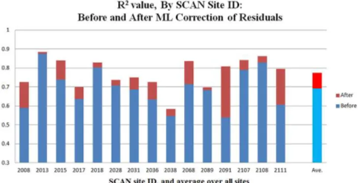
Figure 2.Improvements from machine learning (KNN) models of residuals.
predictions at site y; the other signifies the performance of parameters calibrated at sitey making predictions at sitex.
At this point, three types of (x, y) pairs emerge. If the hypothesis is correct, then the first type, when x andy fall within the same hydroclimatic class, should display limited losses in predictive power. The second type, when x andy
fall within a “similar” hydroclimatic class (two classes dif-fering by a single division of the classification tree developed in Coopersmith et al., 2012), should display greater losses of predictive power. Finally, the third type, when x andy fall in two unrelated classes, should display the largest loss of predictive power.
2.4 Step 4: estimation by hydroclimatic and edaphic similarity
The final step extends the hypothesis proposed in step 3 by evaluating the impacts of soil texture and type on soil mois-ture predictive power. The 15 sites from SCAN are examined based upon the soil textural information available from the pedon soil reports that SCAN provides, as well as data from the Natural Resources Conservation Service’s (NRCS) soil survey database1.
This information allows sites already deemed hydrocli-matically similar to be further subdivided into sites that are and are not edaphically similar. Analogous to the previous section, we consider pairs of sites,x andy, where parame-ters are calibrated at sitexand validated at sitey. In this case, four groups can be defined – the first, wherexandyand hy-droclimatically similar; the second, wherexandyare hydro-climatically similar but differ edaphically; the third, wherex
and y are edaphically similar but differ hydroclimatically; and, finally, wherexandy are hydroclimatically and edaph-ically dissimilar.
1http://websoilsurvey.sc.egov.usda.gov/App/WebSoilSurvey.
aspx.
3 Results
This section begins by presenting the results of the machine learning approach used in error correction during the ini-tial calibration step (Sect. 3.1). Next, Sect. 3.2 presents re-sults for the hydroclimatic similarity analysis, illustrating the performance of calibration–validation pairs within the same class and without. Finally, Sect. 3.3 shows how the predic-tive power improves when both hydroclimatic and edaphic similarity are considered.
3.1 Testing the value of machine learning error correc-tion for soil moisture prediccorrec-tion using the diagnostic soil moisture equation
Figure 2 shows the performance of the calibrated parame-ters for the 15 SCAN sites using only the diagnostic soil moisture equation (step 1 of the methodology) along with the subsequent improvement in performance following ma-chine learning error correction (step 2). In each case, the six parameters required for the implementation of the diagnos-tic soil moisture equation are calibrated using training data from before 2010. Sensors with hourly precipitation and soil moisture time series data between 2004 and 2009 (inclusive) provide 4 to 6 years of training data (some sites are missing 1 or 2 years of data). Only days of the year where snow cover is unlikely are used to train the algorithm (from the 100th to 300th day of the year in all locations, for consistency). Vali-dation data consist of days 100–300 for 2010 and 2011.
The results illustrate that, in all 15 test cases, performance within the validation sample is improved by machine learn-ing modellearn-ing of residuals from the trainlearn-ing set; in some cases, as much as 26.9 % of the unexplained variance (site 2091) in soil moisture is corrected from by this technique. The average results (far right column, Fig. 2) illustrate that the diagnostic soil moisture equation explains just 69.2 % of the variance in soil moisture (ρ=0.83) before machine learning corrections occur, but explains 77.5 % of the vari-ance in soil moisture (ρ=0.88) thereafter.
Figure 3.Soil moisture time series, SCAN site 2015, New Mex-ico (USA), actual soil moisture (blue line), diagnostic soil moisture equation estimate (red line), and diagnostic soil moisture equation with machine learning error correction (green line). Hydroclimate: IAQ (intermediate seasonality, arid, summer peak runoff). Soil tex-ture: loamy sand.
Figure 4.Soil moisture time series, SCAN site 2068, Iowa (USA), line colors from Fig. 3. Hydroclimate: ISCJ (intermediate seasonal-ity, semi-arid, winter peak runoff, summer peak precipitation). Soil texture: silty clay loam.
precipitation during February or March), and Cold runoff. Using error correction models for prediction at these sites in-creasedR2values by an average of 8.2 %, which is similar to the 8.3 % improvement inR2averaged across all 15 sites. Thus, these three locations are representative in terms of both hydroclimatic and edaphic diversity and their responsiveness to machine learning.
The base soil moisture model results from applying step 1 at the three sites are displayed in Figs. 3–5. These predic-tions are shown with the results produced by deploying the machine learning algorithm (KNN) in step 2 to remove bias and correct errors. In each image, the blue line represents the observed soil moisture readings, the red line represents the estimates generated by the diagnostic soil moisture equation, and the green line represents those predictions after the ma-chine learning algorithm has removed biases and corrected errors. Soil moisture values (y axis) are presented as volu-metric percentage (0–100).
In Fig. 3, the diagnostic soil moisture equation is able to trace the general trend of the soil moisture time series (ρ=0.860). However, during the middle of the time series, in which the observed soil moisture values fall below 5 %, the
Figure 5. Soil moisture time series, SCAN site 2013, Georgia (USA), line colors from Fig. 3. Actual soil moisture (blue line), diagnostic soil moisture equation estimate (red line), and diagnostic soil moisture equation with ML error correction (green line). Hy-droclimate: LWC (low seasonality, winter peak precipitation, winter peak runoff). Soil texture: sandy loam.
benefits of machine learning error correction are most note-worthy. There are other hours scattered throughout the data set where the green line (prediction with machine learning) follows the blue line (observed values) much more closely than the red line (diagnostic soil moisture equation). The green line (ρ=0.917) not only improves upon the correla-tion value of Pearson’s Rho (the square root of theR2value in Eq. 5), but also displays marked improvement for those cases in which the diagnostic soil moisture equation produces significant errors.
During the validation period, specifically 2010, wetter conditions were observed than were present during calibra-tion. At this SCAN site, before 2010, the average soil mois-ture value observed was 28.55 %, with only 25 % of val-ues exceeding 35 % volumetric soil moisture. However, in 2010, the average soil moisture value measured was 33.16 % with 45 % of values exceeding 35 %. The machine-learning-driven error correction improves the diagnostic soil moisture equation (ρ=0.846) significantly (ρ=0.915), but fails to raise its forecasts to reach some of the wetter conditions ex-perienced in validation. Underestimations of this nature, al-though detrimental in terms of numerical errors, are not nec-essarily a problem for decision support of agricultural or con-struction activities, for example. If a model warns that a site is very wet and in reality it is even wetter than predicted, the user has still been given adequate warning not to attempt activity at that site. It is important to note that small errors are more significant in terms of decision support (specifically when and where to irrigate) during dry conditions. Generally, the model’s errors are smaller, in absolute terms, during drier conditions. This analysis’s approach to error correction, as it relies on previous errors to predict future errors, will not address long-term trends within the soil moisture record.
Figure 6.Soil moisture time series, SCAN Site 2015, New Mex-ico (USA), actual soil moisture (blue line), diagnostic soil moisture equation estimate (red line), and diagnostic soil moisture equation with machine learning error correction (green line).
improvement (ρ=0.941). It is worth noting that machine learning does not damage an already excellent performance, offering slight improvements when possible and essentially no correction when training data suggest the model has al-ready performed adequately.
Table 1 presents all 15 sites for which the diagnostic soil moisture equation has been calibrated, including informa-tion regarding their hydroclimatic class from Coopersmith et al. (2012), their soil textural characteristics, and their perfor-mance before and after the KNN bias correction process. 3.2 Bias correction – more detailed results
In addition to generalizing the parameters calibrated in the diagnostic soil moisture equation, the error correction ap-proach allows for systematic biases to be removed by search-ing trainsearch-ing data for similar conditions and then predictsearch-ing the types of mistakes most likely to occur. Figure 6, by zoom-ing in upon a 30-day period from Fig. 2, illustrates how ma-chine learning reduces errors by introducing a diurnal cycle into a model that previously lacked one. The remaining bias is likely explained by a slightly wetter training data set as compared with the validation data. It is possible that the di-urnal cycle at some locations reflects a soil moisture probe’s dependency on electromagnetic properties driven by temper-ature change (apparent permittivity) rather than hydrologic processes (Rosenbaum et al., 2011). However, the model’s ability to respond to these nuances would not compromise its performance were these nuances subsequently removed.
Any corrective algorithm will, over thousands of valida-tion points, push the estimate away from the observed value in some cases. However, the results from Table 1 demon-strate that its overall performance represents an improvement at all sites, and thereby justifies its use. Regarding the issue of “measurement artifacts”, whether the diurnal cycle is gen-uine or an idiosyncratic sensor output, the model is tasked with calibrating itself and correcting biases as defined by the empirically reported data. Figure 6 illustrates its ability to do so. Were the sensors to no longer report such a
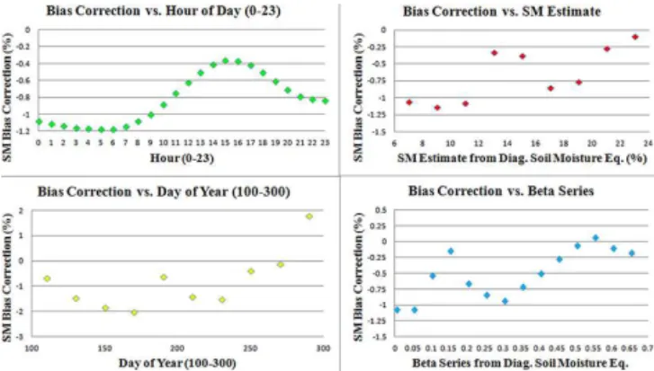
di-Figure 7.Bias correction analysis, SCAN site 2015 (IAQ, desert, loamy sand).
Figure 8.Bias correction analysis, SCAN site 2068 (ISCJ, plains, silty clay loam).
urnal pattern (i.e., it is merely a measurement artifact, and subsequently corrected), the machine learning step would no longer observe those biases and, consequently, no longer in-troduce such a pattern. The accuracy of SCAN is a relevant inquiry, but unfortunately not within the scope of this paper. By addressing such systematic biases, machine learning enables model performance to improve with each succes-sive growing season as the training data set expands. For instance, although the fields in Iowa endured flooding dur-ing the validation period and subsequently made errors, such errors would eventually populate the training data. The next time such flooding occurs, the model is likely to recognize the occurrence of those same conditions and adjust the di-agnostic soil moisture equation’s predictions accordingly. In this vein, model performance is likely to improve over time, especially with the models already showing reasonable accu-racy using only a few years of training data.
Table 1.The 15 SCAN sites: class and soil information and performance.
Hydro- RMSE R2
Site ID climate Soil information RMSE w/ KNN R2 w/ KNN 2008 LJ Sandy loam 8.38 7.69 0.590 0.726 2013 LWC Sandy loam 2.16 2.06 0.876 0.885 2015 IAQ Loamy sand 3.29 2.37 0.740 0.841 2017 ISQJ Sandy loam 3.62 3.27 0.637 0.701 2018 IAQ Loamy sand* 2.23 2.16 0.803 0.828 2028 LPC Loam 4.89 4.71 0.707 0.738 2031 ISQJ Silty clay loam 5.46 6.00 0.687 0.750 2036 LPC Silt loam 4.61 3.95 0.635 0.726 2038 LJ Sandy loam 4.81 4.51 0.546 0.584 2068 ISCJ Silty clay loam 5.28 4.03 0.716 0.837 2089 LJ Sandy loam 6.7 6.31 0.682 0.697 2091 LPC Silt 8.12 6.89 0.539 0.808 2107 IAQ Loamy sand 1.98 1.85 0.790 0.843 2108 IAQ Loamy sand/sand 1.26 1.12 0.828 0.863 2111 ISQJ Silty clay loam 5.38 5.01 0.607 0.796
* Not similar to other sandy soils; see Fig. 12.
Figure 9.Bias correction analysis, SCAN site 2013 (LWC, woods, sandy loam).
of hydroclimatic and edaphic conditions. The upper-right im-age of each figure presents the bias correction as a function of the unadjusted soil moisture estimate – essentially, whether there exists a systemic over- or underestimation when values are high or low.
The first two sites (Figs. 7 and 8) do not present a clear pattern, but Fig. 9 displays a trend suggesting that the high-est high-estimates of soil moisture tend to be overhigh-estimates and the lowest estimates of soil moisture tend to be underesti-mates – but these biases are removed via machine learning. The lower-left image presents bias correct as a function of the day of the year (from 100 to 300, the days of the year when the model is applied). At all three sites, the seasonal cycle does appear in terms of the patterns of bias correction, but the pattern is noisier than the diurnal cycle. The magnitudes of the adjustments are largest in the monsoon-affected desert of New Mexico, a bit smaller in the Midwestern plains
char-acterized by less extreme seasonal behavior, and smallest in the southeast where seasonal variations are low.
Finally, the lower-right image relates bias correction to the beta series from the diagnostic soil moisture equation (Pan, 2012), a convolution of a decaying precipitation time series working backwards temporally from the current time. Stated differently, these charts relate bias correction to the amount of antecedent precipitation (with more recent pre-cipitation weighted more heavily). In Fig. 7 (plains, silty clay loam), the model tends to underestimate moisture when large quantities of antecedent rainfall are present, where in Fig. 9 (woods, sandy loam), once antecedent precipitation becomes non-trivial, the opposite pattern is displayed. This is consistent with the finer Midwestern soils’ proclivity for ponding/flooding due to larger proportions of clay. In these cases, larger amounts of rain will soak soils from above, and capillary rise might further soak sensors from below, leading to underestimation from the diagnostic soil moisture equa-tion and subsequent machine learning correcequa-tion. By con-trast, with sandier soils, drainage occurs easily, leading to higher rates of loss than the eta series (Pan, 2012) would pre-dict (there is more available water to lose), leading to over-estimation with large amounts of antecedent rainfall.
3.3 Cross-validation results for hydroclimatic similarity: qualitative findings and significance testing
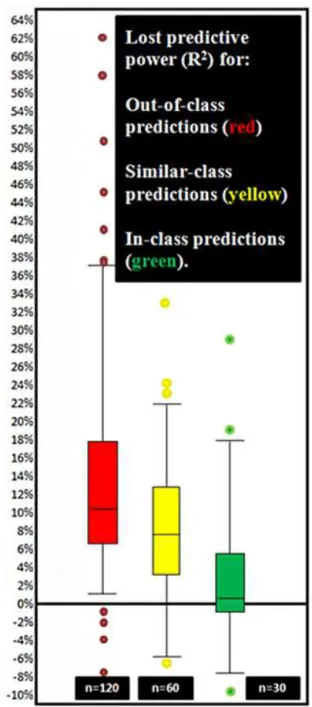
Figure 10. Loss of predictive power (R2) (yaxis) between base-line predictions (model calibrated in the same watershed) and cross-validation predictions (model calibrated in other watersheds).
level of performance for a given site (validation performed using the parameters calibrated at that same location). Of the 210 remaining(x, y)pairs, 120 of them consist of paired catchments in whichxandyare located in unrelated classes, 60 consist of paired catchments in whichxandyare located in a similar class (different by a single split within the clas-sification tree), and 30 consist of paired catchments in which
x andy fall within the same hydroclimatic class (butx and
y do not represent the same catchment). Figure 10 presents box plots illustrating the change inR2values for these three sets of pairs in a manner analogous to the differences shown
Table 2.Cross-validation results.
Unrelated Similar Same class class class Median −10.5 % −7.3 % −0.8 % Mean −13.7 % −7.7 % −3.4 % Standard deviation 1.0 % 1.1 % 1.4 %
Figure 11.428 MOPEX catchments colored by hydroclimatic class (Coopersmith et al., 2012). Fifteen SCAN sensors (for which the diagnostic soil moisture equation is calibrated) are shown as colored circles. Circle colors correspond to the hydroclimatic class of the point in question. Circles with dotted borders are unique (no other sensor for calibration is available within that class).
in Fig. 2. Table 2 presents the quantitative results, again av-eraging the deterioration of performance in terms of change inR2.
These findings show that calibrating the model at one lo-cation and applying those parameters elsewhere within the same class (green) is preferable to applying those parameters in a similar, but not identical, class (yellow) and vastly supe-rior to applying those parameters in an unrelated class (red). The differences between any two clusters (same class, sim-ilar class, unrelated class) are all significant at theα=0.01 level (p < .001 in all cases) as calculated by a two-sample, heteroscedasticttest (Welch, 1947).
3.4 Impact of soils: cross-validation results for edaphic and hydroclimatic similarity
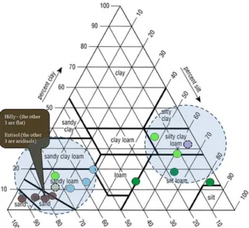
Figure 12.The 15 SCAN sensors, color-coded to match their hy-droclimatic class, with similar soil textures shaded.
was unavailable, from soil information in the national soil Web database2.
Of the 13 sensors from the 4 hydroclimatic classes with multiple SCAN sensors (light green, blue, dark green, and brown in Figs. 11 and 12), 30 (x, y) pairs exist where the model can be calibrated at sitex and its parameters applied at site y. Note that (x, y) is not equivalent to (y, x) as the sites for calibration and validation are reversed. Of these 30 pairs, 20 pairs are edaphically similar as well. However, 10 of them include a pair of points where the soil types or terrain types are notably misaligned (for example, light green dots in Fig. 12 where two of the three sensors are in silty clay loam and the third is in sandy loam – notably different soil). A similar analysis to the one presented in Fig. 10 and Table 2 has been reproduced, comparing the loss in predictive power (R2)for the 20 pairs with similar hydroclimates and soils against the loss for the 10 pairs in which either the soil texture (Fig. 12) or type does not align. The average loss of 1.0 % for the 20 very similar pairs is a much smaller decline than the 8.0 % average decline observed for the 10 pairs for which soil/terrain information suggests dissimilarity. These results are significant, with apvalue of approximately 0.02. Addi-tionally, the uppermost two green dots in Fig. 10, where cal-ibrated parameters at one location perform poorly at another of similar hydroclimatic class, fall within these 10 cases.
These observations show the importance of soil infor-mation, or edaphic similarity. While pairs of calibration– validation locations with similar hydroclimates, but dissim-ilar soils, show a decline in performance as compared with pairs of locations where both are similar, so too do
loca-2http://websoilsurvey.nrcs.usda.gov/app/WebSoilSurvey.aspx
Figure 13.Venn diagram of modeling errors with similar and dif-ferent soils and hydroclimates.
tions with similar soils but dissimilar hydroclimates. The shaded circles in Fig. 12 illustrate groups of sensors that are quite similar in terms of soil textures. However, despite their soil similarities, differences in hydroclimates hinder cross-application, showing a decline in performance of 10.9 % for all (x, y) pairs within the shaded regions of Fig. 12 for which
xandyare not from the same hydroclimatic class.
As summarized in Fig. 13, these results suggest that, in cases where both soil type and hydroclimate align, very little performance is lost when parameters are re-applied (1.0 %), moderate declines in performance are observed when one of these two factors is aligned (8.0 % if hydroclimates align and soil types do not; 10.9 % if soil types align but hydroclimates do not), and large declines in performance appear when nei-ther align (20.5 %). Clearly both types of attributes are im-portant and should be considered in future modeling work in which the relative importance of hydroclimates and soil textures can be examined in greater detail.
4 Discussion: future work to improve predictions
This section discusses other approaches that could be used in the future to improve and broaden the applicability of the methods developed in this work. First, we will consider micro-topographic effects on soil moisture, as local peaks and valleys can cause soils to dry more or less rapidly. Sec-ond, we will discuss a conceptual omission within the diag-nostic soil moisture equation – infiltration excess. Finally, we will discuss the role of future satellite data on soil moisture modeling.
4.1 Estimates enhanced by topographic classification
lumped, bucket model is not ideally suited for landscapes with complex topography. Conveniently, the majority of SCAN sites are placed on relatively flat surfaces. Integra-tion of topographic insights is a fertile area for future re-search. One possible approach to further improving predic-tive accuracy is to disaggregate the soil moisture estimates as a function of local topography. While SCAN sites used for soil moisture data are generally located on flat surfaces, pre-dictions may be needed at locations located on ridges or in valleys where the soils are likely to be wetter or drier than their surroundings. This requires the notion of regional topo-logical classification. In this manner, the notion of similarity is extended to include hydroclimatology, soil characteristics, and topographic designation (ridge, slope, valley, etc.). Pre-liminary analyses suggest that small-scale topography does play a meaningful role in the wetting–drying process. Future research with more extensive data sets in locations with more complex topological contours could improve soil moisture predictions by enabling the models developed in this work to be adjusted as a function of local topographic classification. 4.2 An enhanced diagnostic soil moisture equation
The diagnostic soil moisture equation could also be improved in future modeling efforts by considering overland and sub-surface flows, specifically in areas characterized by more complex topography. Currently, the model assumes that, in the absence of saturation, all rainfall will ultimately infil-trate, as the porosity parameter serves as an upper bound on soil moisture levels. The diagnostic soil moisture equation was designed originally as a daily model, and it is proba-bly rare that on any given day a significant fraction of pre-cipitation does not infiltrate. However, at the hourly scale it is quite possible that the water from an intense rainfall event will not make its way into the soil at the location of the sensor. To address this lateral transfer phenomenon, ad-ditional parameters can be introduced into the diagnostic soil moisture equation that place an upper bound on the quan-tity of rainfall that can be infiltrated during any hour (or other interval) of the convolution calculation for any partic-ular soil type. Agricultural decision support includes traffi-cability when wet (Coopersmith et al., 2014) and irrigation support when dry. While overland flow is perhaps an un-needed component in water-limited catchments where irri-gation schemes represent the most significant soil-moisture-related decision, in wetter catchments, in which trafficability is a real concern, such an addition could improve the model. While this approach would require the fitting of additional parameters, it is likely that predictions would be improved. These additional parameters could also be considered in as-sessing cross-site edaphic similarity using the methods de-scribed above, although they may be highly correlated with existing parameters such as porosity, residual soil moisture, and drainage.
4.3 Water balance models and up-scaling
The diagnostic soil moisture equation used in this paper (Pan et al., 2003; Pan, 2012) was an appropriate choice due to its ability to generate soil moisture estimates without the need for knowledge of antecedent soil moisture conditions. Koster and Mahanama (2012) and Orth et al. (2013) have devel-oped approaches to estimate soil moisture at the watershed scale by leveraging hydroclimatic variability and long-term streamflow measurements in a water-balance model – also without employing previous soil moisture conditions. If the parameters calibrated and then generalized in this work pro-duce point estimates of soil moisture at a diversity of loca-tions, integration with a water balance approach could help with the up-scaling process.
5 Conclusions
This work has demonstrated the feasibility of estimating soil moisture at locations where soil moisture sensors are unavail-able for calibration, provided they fall within hydroclimati-cally and edaphihydroclimati-cally similar areas to gauged locations. By calibrating the diagnostic soil moisture equation via a two-part genetic algorithm, improving its performance via a ma-chine learning algorithm for error correction, then validating that algorithm at the same location in subsequent years, a baseline level of predictive performance is established at 15 locations. Next, these results are cross-validated – deploy-ing parameters calibrated at a given site at sites of similar and different hydroclimatic classes, demonstrating that pa-rameters can be re-applied elsewhere within the same class, but not without. Finally, by incorporating edaphic informa-tion, we observe the strongest cross-validation results when hydroclimatic and edaphic characteristics align. As only 24 hydroclimatic classes describe the entire nation (and only 6 describe a significant majority), it is entirely possible that a couple dozen well-placed soil moisture sensors can enable reasonably accurate soil moisture modeling at any location within the contiguous United States.
It is likely that the types of errors made when parameters are cross-applied between sites of different hydroclimates will differ from the types of errors that appear when the sites differ edaphically. Further research extending beyond model performance into the specific conditions under which mod-els perform less effectively along with the magnitude and bias of those errors would be highly illustrative for future researchers.
for satellite estimates of soil moisture. Scaling these results downward can help maximize yields. Given the ubiquity of precipitation data, which are the only inputs these models require, better understanding of the transferability of mod-eled parameters is a step towards far-wider availability of soil moisture estimates.
Leveraging these findings, the discussion section also pre-sented the results of preliminary analysis that illustrates how further improvements in soil moisture predictions could be gained by disaggregating based on local topography. This would enable more accurate predictions at sites character-ized by peaks and valleys that dry faster or slower than the relatively flat locations at which soil moisture algorithms are generally calibrated. Incorporating overland flow into the di-agnostic soil moisture equation and integrating satellite data into the approach could also improve predictions in the fu-ture.
Acknowledgements. We appreciate the thoughtful commentary of the reviewers – the paper is unquestionably enhanced by their insights. We would also like to acknowledge professors Praveen Kumar and Carl Bernacchi at the University of Illinois, whose perspectives were beneficial in considering soil textural properties. Edited by: N. Romano
References
Barricelli, N. A.: Numerical testing of evolution theories. Part II. Preliminary tests of performance, symbiogenesis and terrestrial life, Acta Biotheoretica, 16, 99–126, 1963.
Capehart, W. J. and Carlson, T. N.: Estimating near-surface soil moisture availability using a meteorologically driven soil water profile model, J. Hydrol., 160, 1–20, 1994.
Cheng, C. T., Zhao, M. Y., Chau, K. W., and Wu, X. Y.: Using Ge-netic Algorithm and TOPSIS for Xinanjiang model calibration with a single procedure, J. Hydrol., 316, 129–140, 2006. Chico-Santamarta, L., Richards, T., and Godwin, R. J.: A laboratory
study into the mobility of travelling irrigators in air dry, field capacity and saturated sandy soils, American Society of Agri-cultural and Biological Engineers Annual International Meeting 2009, Vol. 4, 2629–2646, 2009.
Choudhury, B. J. and Blanchard, B. J.: Simulating soil water reces-sion coefficients for agricultural watersheds, Water Resour. Bull., 19, 241–247, 1983.
Coopersmith, E., Yaeger, M. A., Ye, S., Cheng, L., and Sivapalan, M.: Exploring the physical controls of regional patterns of flow duration curves – Part 3: A catchment classification system based on regime curve indicators, Hydrol. Earth Syst. Sci., 16, 4467– 4482, doi:10.5194/hess-16-4467-2012, 2012.
Coopersmith, E. J., Minsker, B. S., Wenzel, C. E., and Gilmore, B. J.: Machine learning assessments of soil drying for agricultural planning, Comput. Electron. Agr., 104, 93–104, doi:10.1016/j.compag.2014.04.004, 2014.
Entekhabi, D. and Rodriguez-Iturbe, I.: Analytical framework for the characterization of the space-time variability of soil moisture, Adv. Water Resour., 17, 35–45, 1994.
Farago, T.: Soil moisture content: Statistical estimation of its prob-ability distribution, J. Clim. Appl. Meteorol., 24, 371–376, 1985. Fix, E. and Hodges, J. L.: Discriminatory analysis, nonparamet-ric discrimination: Consistency properties. Technical Report 4, USAF School of Aviation Medicine, Randolph Field, Texas, 1951.
Gamache, R. W., Kianirad, E., and Alshawabkeh, A. N.: An automatic portable near surface soil characterization system, Geotechnical Special Publication, Issue 192, 89–94, 2009. Goldberg, D. E.: Genetic Algorithms in Search, Optimization, and
Machine Learning, Addison-Wesley Professional, 1989. Jackson, T. J., Bindlish, R., Cosh, M. H., Zhao, T., Starks, P.
J., Bosch, D. D., Seyfried, M., Moran, M. S., Goodrich, D. C., Kerr, Y. H., and Leroux, D.: Validation of soil moisture and ocean salinity (SMOS) soil moisture over watershed networks in the U.S., IEEE Trans. Geosci. Remote Sens., 50, Part 1, 1530– 1543, May, 2012.
Jones, H. G.: Irrigation scheduling: advantages and pitfalls of plant-based methods, J. Experiment. Botany, 55, 2427–2436, 2004. Koster, R. D. and Mahanama, S. P. P.: Land Surface Controls on
Hydroclimatic Means and Variability, J. Hydrometeor, 13, 1604– 1620, doi:10.1175/JHM-D-12-050.1, 2012.
Orth, R. A., Koster, R. D. B., and Seneviratne, S. I. A.: Inferring soil moisture memory from streamflow observations using a simple water balance model, J. Hydrometeor., 14, 1773–1790, 2013. Pan, F.: Estimating daily surface soil moisture using a daily
diagnos-tic soil moisture equation, J. Irrig. Drainage Eng., 138, 625–631, 2012.
Pan, F. and Peters-Lidard, C. D.: On the relationship between the mean and variance of soil moisture fields, J. Am. Water Resour. Assoc., 44, 235–242, 2008.
Pan, F., Peters-Lidard, C. D., and Sale, M. J.: An analytical method for predicting surface soil moisture from rainfall observations, Water Resour. Res., 39, 1314, doi:10.1029/2003WR002142, 2003.
Rosenbaum, U., Huisman, J. A., Vrba, J., Vereecken, H., and Bogena, H. R.: Correction of temperature and electri-cal conductivity effects on dielectric permittivity measure-ments with ECH2O Sensors, Vadose Zone J., 10, 582–593, doi:10.2136/vzj2010.0083, 2011.
Saxton, K. E. and Lenz, A. T.: Antecedent retention indexes predict soil moisture, J. Hydraul. Div. Proc. Am. Soc. Civ. Eng., 93, 223– 241, 1967.
Schaefer, G. L., Cosh, M. H., and Jackson, T. J.: The USDA Natural Resources Conservation Service Soil Climate Analysis Network (SCAN), J. Ocean. Atmos. Technol., 24, 2073–2077, 2007. Simunek, J., Sejna, M., and van Genuchten, M.: The HYDRUS-1D
software package for simulating water flow and solute transport in two-dimensional variably saturated media, Version 2.0, IG-WMC – TPS – 70, International Ground Water Modeling Center, Colorado School of Mines, Golden, CO, 1998.
Singh, A. and Minsker, B. S.: Uncertainty-based multiobjective optimization of groundwater remediation design, Water Resour. Res., 44, W02404, doi:10.1029/2005WR004436, 2008. Steel, R. G. D. and Torrie, J. H.: Principles and Procedures of
Wetzel, P. J. and Chang, J. T.: Evapotranspiration from nonuniform surfaces – A 1st approach for short-term numerical weather pre-diction, Mon. Weather Rev., 116, 600–621, 1988.