A multi channel coupling based approach for the prediction of the channel capacity of MIMO-systems

www.adv-radio-sci.net/9/153/2011/ doi:10.5194/ars-9-153-2011

© Author(s) 2011. CC Attribution 3.0 License.

Radio Science

A multi channel coupling based approach for the prediction of the

channel capacity of MIMO-systems

F. Hageb¨olling and U. Z¨olzer

Department of Signal Processing and Communications, Helmut Schmidt University – University of the Federal Armed Forces Hamburg, Holstenhofweg 85, 22043 Hamburg, Germany

Abstract. When installing Multiple Input Multiple Output (MIMO)-systems, the antenna positioning has a major influ-ence upon the achievable transmission quality. To determine those antenna positions, which maximize the transmission quality, in adequate time, a computer based prediction of the channel capacity is imperative.

In this paper, we will show that Ray Tracing, which is a very popular prediction method and well suited for the pre-diction of transfer functions or power delay profiles, pro-duces unacceptable errors when predicting the channel ca-pacity of MIMO-systems. Furthermore we identify the source of the prediction errors and present a new algorithm, based on an approach known as Multi Channel Coupling (MCC), which avoids this error source.

Finally a comparison of the prediction results of our al-gorithm with prediction results gained with an Image Ray Tracer as well as with measured results is used to show the formidable increasement of prediction accuracy which can be gained by using our algorithm.

1 Introduction

In Foschini and Gans (1998) it was shown, that MIMO-systems using spatial multiplexing increase the channel ca-pacity to such an extent, that an immensely higher spectral efficiency becomes possible.

When installing such MIMO-systems the count of posi-tions, where antennas can be placed, is usually higher than the number of antennas, which are to be placed. Being aware of the fact, that the antenna positioning has a big impact on the spatial multiplexing capabilities of the MIMO-system and thereby the achievable transmission quality, a lot of effort

Correspondence to:F. Hageb¨olling (falko.hageboelling@hsu-hh.de)

has already been taken to find antenna positionings which maximize transmission quality.

A lot publications concentrate on measuring channel ca-pacities for different positionings in certain scenarios, Tang and Mohan (2005) and F¨ugen et al. (2002) shall be men-tioned exemplarily. But measuring based approaches are al-ways limited by the fact, that the number of possible MIMO-systems increases very fast with the number of possible an-tenna positions.

To be able to compare several thousand or more possi-ble systems, computer based simulation is needed. In Talbi (2001) and Ziri-Castro et al. (2005) and a lot of other publi-cations the received power was predicted and compared with measurements.

Though the results presented in those publications ac-cord very well with measurements, the received power is, in our opinion, not a sufficient quantity to judge the transmis-sion quality of MIMO-systems, because it doesn’t contain any information about the linear independence of the Multi-ple Input Single Output (MISO)-systems contained in each MIMO-system. The latter is important, because in a spatial multiplexing MIMO-system the received signals can only be decoded properly, if the MISO-systems are linearly indepen-dent.

Though the channel capacity contains this important infor-mation only a comparatively small amount of publications deals with the prediction of this quantity. And most of the publications, which do so, don’t present measurements as comparison for the prediction results. Elnaggar et al. (2004) may be named as example.

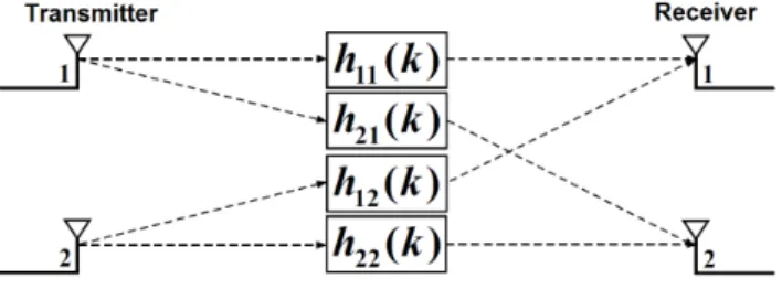
Fig. 1.SISO impulse responses of a MIMO Channel,nT=nR=2

2 Fundamentals 2.1 Channel description

The MIMO Channel withnT transmit antennas and nR

re-ceive antennas consists of one complex Single Input Single Output (SISO) impulse response between every transmit an-tennamand every receive antennan(see Fig. 1).

Assuming the same order L for each of these impulse responseshn,m=hn,m(0) hn,m(1) ... hn,m(Ln,m)T the fre-quency selective MIMO channel can be described byL+1 complex channel matricesH(k)withk=0,...,L:

H(k)=



 

h1,1(k) ··· h1,nT(k)

..

. . .. ...

hnR,1(k)··· hnR,nT(k)





. (1)

2.2 Channel capacity

Assuming that no power allocation strategy is used, the trans-mitted powerPTis uniformly distributed over the bandwidth

Band the Channel Capacity of a frequency selective MIMO system can be written as (Palomar et al., 2000)

C=

Z +B/2

−B/2

log2

det

Im+PT/(nT·B) Snn(f )

Q(f )

df, (2)

withSnn(f )being the power spectral density matrix of the noise,m=min(nT,nR)and

Q(f )=

HF(f )HF(f )H , nR< nT

HF(f )HHF(f ) , nR≥nT

. (3)

Discretizing this equation, assuming additive white noise and normalizing channel energy according to Bauch and Al-Dhahir (2002)

L

X

k=0

Enhn,m(k)

2o

=1 ∀1≤m≤nT,1≤n≤nR (4) leads to the formula

C= 1

NF

NF X

f=1

log₂

det

Im+ ρ

nT

Q(f )

, (5)

withNFbeing the number of discrete frequencies andρ

be-ing the mean Signal to Noise Ratio (SNR).

0 5 10 15 20 25

0 10 20 30 40

placing in predicted order

Capacity / (bit/s/Hz)

27 Scenarios without LOS, results of IRT

measured IRT

RMSE:

IRT: 10,8 bits/ (s * Hz)

Fig. 2.Prediction results gained with image ray tracing.

The normalization according to Eq. (4) is needed to re-place the term PT/(nT·B)

Snn(f ) byρ, but it abolishes differences in the path loss of the SISO-channels and reduces the compa-rability of different MIMO systems. To maintain the differ-ences and to enable a comparison ofNMMIMO systems the condition has to be relaxed to be (Hageb¨olling et al., 2006)

NM

X

i=1

nT X

m=1

nR X

n=1

L

X

k=0

Enh(n,m)i(k)

2o

=NM·nT·nR. (6)

3 Image Ray Tracing

In Hageb¨olling et al. (2006) we presented a prediction algo-rithm based on the very popular method of Image Ray Trac-ing (IRT). The algorithm determines all possible paths be-tween each pair of transmit and receive antennas in a given scenario and with a given number of maximal reflections per path. It then identifies the points, where rays following these paths interact with the surrounding and calculates the im-pact of these interactions upon the electromagnetic field. We showed that the prediction of the channel capacity using this algorithm is in general very accurate but produces certain dis-crepancies for some scenarios.

Figure 2 shows some actual predictions of this algorithm for 27 indoor scenarios. The measurement of the channel capacity of this scenarios has been done using our laboritory MIMO system presented in Weikert and Z¨olzer (2005). In all scenarios there arenT=4 transmit antennas andnR=4

receive antennas, the carrier frequency is 2.49 GHz and the SNR amounts 30 dB.

Especially for the systems number 4, 5, 13, 14 and 15 the prediction error is very high.

Due to their low damping those paths imperatively have to be considered when calculating the impulse response, but because of their high number of reflections they were not considered by the algorithm. This error source is inherent for ray tracing based algorithms and can only be bated by increasing the maximum number of reflections per path.

However this measure does not solve the problem gener-ally and is very expensive in terms of computation time and needed memory, because the complexity of Ray Tracing is of the orderwRforwwalls and a maximal number of reflec-tions per pathR.

4 Multi Channel Coupling

Multi Channel Coupling (MCC) is a prediction algorithm, which takes an infinite number of interactions per path into account. It thereby avoids the mentioned error source, which is inherent for Ray Tracing based algorithms. MCC was first presented as algorithm to predict the transmission of power in 2-D-scenarios in Liebendorfer and Dersch (1997). This algorithm is based upon the following considerations:

– For every pair of walls there are two channels, one in each direction.

– Transmit antennas couple a certain percentage of their transmitted power into each channel.

– Each channel couples a certain percentage of the present power into each other channel.

– Each channel couples a certain percentage of the present power into each receive antenna.

Each coupling of transmit antennas into channels includes one reflection at or transmission through the start wall of the channel and each coupling from a channel into another channel is a reflection or transmission. Every coupling is described by a coupling factor between 0 and 1 and the cou-pling factors are organized in matrices: a(nC×nT)matrixT for the coupling factors of thenTtransmit antennas into the

nCchannels, a(nC×nC)matrixCfor the coupling factors of channels into each other and a(nR×nC)matrixRfor the coupling factors of the channels into thenRreceive antennas. Assuming no direct component and considering an infinite number of couplings from channels into channels, i.e. an infi-nite count of reflections and transmissions, the power transfer matrix from the transmit antennas to the receive antennas can then be calulated by the equation

P=R· T+CT+C2T+ ··· +C∞T

=R·P∞

i=0CiT=R·(I−C)−1T

. (7)

Thus MCC considers an infinite number of reflections and transmissions with the computation time being finite. More-over the most computation time is needed for the calculation

c

b A

P

n c

→

_c XTj

xc

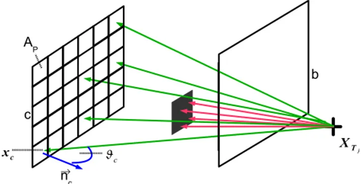
Fig. 3. Coupling from antennaj into channeli; green rays con-tribute to the coupling factor.

of the matrix(I−C)−1, which only depends on the location and the material parameters of walls in the surrounding. Thus MCC is very effective, when calculating the same scenario several times with different antenna positions.

It was already shown, that the MCC method can also be used to predict other values than power. In Karthaus (2001) it was used to predict power delay profiles in 3-D-scenarios. To be able to predict the channel capacity of frequency selective MIMO systems with and without line of sight using the MCC method, we write Eq. (7) as

H(f )=R(f )·(I−C(f ))−1T(f )+D(f ) (8)

withf being the frequency,H(f )being the complex trans-fer function in the frequency domain and the(nR×nT) ma-trixD(f )containing the coupling factors of the direct paths between each pair of transmit and receive antennas.

In the following we will present our formulas for the pre-diction of the channel capacity with Eq. 8.

4.1 The elements of the matrix T(f )

The elementTij describes, how an impulse at the transmit antennaj is coupled into channeli.

To calculateTij, the end wall of channeliis discretized. Then for each raypfrom the transmit antennaTjthrough one of the discrete wallelements with the areaAcit is calculated, how the amplitude and the phase of an impulse transmitted by the antenna is altered by the coupling.

Only rays, which intersect with the start wall of the chan-nel and are not disturbed by other walls can contribute to the coupling factor. The impact on the amplitude is represented byτpand calculated using the portion of the solid angle, un-der which the wallelement is seen from the position of the transmit antenna, the antenna gainGjand the absolute direc-tional characteristicCj,p

of the antenna at pathp and the

transmission / reflection coefficientrp(f )at the start wall of the channel. The superposition of all rays yields the absolute value of the coupling coefficient.

b A

P

A P

a c

n c

→

n b

→

n a

→

b

c

_a

x_c

x_b

x

a

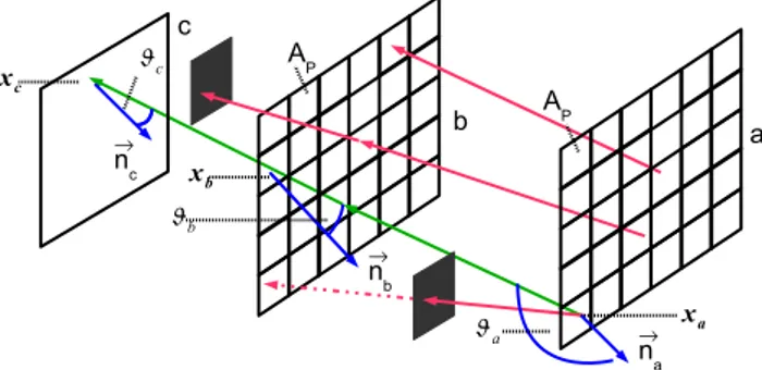
Fig. 4. Coupling from channelj into channeli; green rays con-tribute to the coupling factor.

ϕ0caused by the free space propagation from the antenna to

the wallelement. The phase of each rayp is weighted with the according valueτp and the mean value of all weighted phases is the phase of the coupling coefficient:

Tij(f )=

s X

p

τp(f )·ej ϕ(f ) (9)

with

τp(f )=11

Ac·cos(ϑc)

x

′ Tj−xC

−2

4π ·Gj

Cj,p

rp(f )

ϕ(f ) =

P

p(arg(rp(f ))+ϕ0p(f ))·τp(f ) P

pτp

11 =







1 if ray fromTjthroughAcandb

is not interrupted 0 else

(10)

4.2 The elements of the matrix C(f )

The elementCij describes the coupling from channelj into channeli and is the expectation value of the ratio between the transfer function in channeliand that one in channelj.

For the calculation, the start and the end wall of channelj

are discretized. Of all rayspα from a discrete wall element of the start walla of channel j through a discrete wall el-ementαof the end wallb of channelj, only those, which hit the end wall of channeliand are not disturbed by other walls, contribute to the coupling. Again the absolute value of the coupling factor is obtained by the superposition of all contributing rays and its phase is the average of the weighted phases of the rays.

The wall element at wallahas the areaAaand is thought of as full radiator, which transmits in every direction pro-portional toAacos(ϑa). The remaining, the coupling coefic-cient defining quantities are the portion of the solid angle, under which the wallelement of wallbis seen from the po-sitionxa and the transmission / reflection coefficient rp(f ) at wallb. For the calculation of all transmission or reflexion coefficients the wave matrix method (Layer, 2001) is used,

which allows the definition of walls with layers of different materials.

Cij(f )=

s _P

α

P

pαXpα

P

α

P

pαχpα(f )

·ej ϕ(f ) (11)

with

χp(f )=11Aacos(ϑa)Abcos(ϑb)|xa−xb|−2

Xp =12χp(f )

rp

ϕ(f ) =

P α

P

pα(arg(rpα(f ))+ϕ0pα(f ))·12χpα(f )|rpα(f )| P

α P

pα12χpα(f )rpα(f )

11 =







1 if line fromAatoAb is not interrupted 0 else

12 =







1 if ray fromAathroughc is not interrupted 0 else

(12)

If the pointsxb andxa are equal, which is possible, if the wallsaandbdo intersect each other, only the portion of the solid angle, under which the wallelement of wallc is seen from the positionxa and the numberNc of rays starting at

xa, which hit wallcare used to calculate the coupling factor.

χpthen isχp=1 and

Xp=

1

Nc

X

p

12Accos(ϑc)|xa−xc|

−2

4π . (13)

4.3 The elements of the matrix R(f )

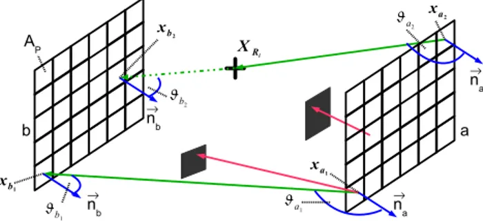
The elementRij describes how the signal is coupled from channelj into the receive antennai. The coupling factor is unequal to zero for all non disturbed raysPα from a discrete wall element of the start wallaof channelj through the po-sition of the receive antenna and a discrete wall elementαof the end wallbof channelj. Every ray is thought of as repre-senting a subchannel of channelj, having the cross section areaAaat walla,ARat the receive antenna andAb at wall

b. The discrete wall element at walla is again thought of as full radiator. The coupling factor is further determined by the portion of the solid angle, under which the wallelement of wallbis seen from the positionxaand the ratio between the cross section areaARand the aperture of receive antenna

Gi|Ci,p|λ2

a b

A

P XRi



a1 

b

1

_b 2

_a 2

n b

→

n b

→

n a

→

n a

→

x_a

1

x_b

1

x_a

2

x_b

2

Fig. 5. Coupling from channelj into antennai; green rays con-tribute to the coupling factor.

Rij(f )=

v u u t

P

α

P

pα11Gi

Ci,p

λ

2

4π ARρα

P

α

P

pα12ρα

·ej ϕ(f ) (14)

with

ρ(f )=Aacos(ϑa)Abcos(ϑb)|xa−xb|−2

ϕ(f )=P

α

ϕ0pα(f )ρpα(f ) P

αρpα(f )

11 =







1 if ray fromAathroughxRi hitsAb without interruption

0 else

12 =







1 if ray fromAahitsAb without interruption 0 else

(15)

Using the intercept theorem one can show that

AR=4

_|

xb−xR| |xa−xb|

2

Aacos(ϑa) (16)

and that leads to a formula for Rij which needs only one summation over all raysrfrom the discrete wall elements of wallato the receive antenna:

Rij(f )=

s _P

rκr

P

α

P

pα12ρα

·ej ϕ(f ) (17) with

κ(f )=11₁₆λ2_πGiCi,pcos(ϑa)|xa−xBS|−2

ϕ(f )=P

r

ϕ0r(f )κr(f ) P

rκr(f )

(18)

andρ,11and12remaining the same as in Eq. (15). 4.4 The elements of the matrix D(f )

The element Dij describes the free space distribution be-tween transmit antenna j and receive antenna i. It is cal-culated as

Dij(f )=

r0

r ·e

−j2_λπ(r−r0) ₍₁₉₎

0 5 10 15 20 25

0 10 20 30 40

placing in measured order

Capacity / (bit/s/Hz)

27 Scenarios without LOS, results of IRT and MCC

MCC measured IRT

RMSE

IRT: 10,8 bits / (s * Hz) MCC: 3,8 bits / (s * Hz)

Fig. 6.Comparison of MCC and IRT.

with r being the distance between the antennas and r0= λ(4π )−1. If the first fresnel zone is not free of obstacles,

Dij is proportional tor−2instead ofr−1, which is known as double regression model.

5 Appraisal of prediction results

Figure 6 shows the results of the prediction of the 27 sce-narios mentioned in Sect. 3 using the new algorithm. For comparison with the results of the Ray Tracing based algo-rithm and the measurements, this data is also shown in the figure. One can see, that the prediction using MCC does not produce the same big errors as that using IRT.

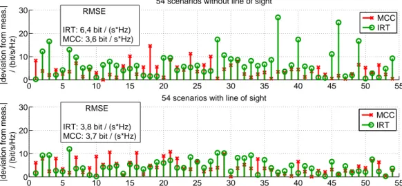
By avoiding the errors, which are inherent to mea-sures, which can only handle a finite count of interac-tions, Multi Channel Coupling outperforms Image Ray Tracing in terms of the root mean square error (RMSE). While the RMSE of the Ray Tracing based prediction amounts up to 10.8 bits (Hz s)−1, MCC has a RMSE of only 3.8 bits (Hz s)−1, which is approximately a third of the first one. To further support the thesis above, Fig. 5 shows the ab-solute deviations of MCC and IRT from measurements for 108 indoor scenarios, 54 with line of sight (LOS) and 54 without one. In a scenario with a line of sight, usually the LOS is the path, where the most power is transfered to the receiver. Concomitantly, the LOS is always taken into recog-nition while the Ray Tracing based prediction, because the number of reflections on that path is zero.

0 5 10 15 20 25 30 35 40 45 50 55 0

10 20 30

|deviation from meas.|

/ (bit/s/Hz)

54 scenarios without line of sight

0 5 10 15 20 25 30 35 40 45 50 55

0 10 20 30

|deviation from meas.|

/ (bit/s/Hz)

54 scenarios with line of sight

MCC IRT MCC IRT RMSE

IRT: 6,4 bit / (s*Hz) MCC: 3,6 bit / s*Hz)

RMSE

IRT: 3,8 bit / (s*Hz) MCC: 3,7 bit / (s*Hz)

Fig. 7.Comparison of MCC and IRT: 108 scenarios.

6 Conclusions

We explained, why in our opinion only the channel capacity is an adequate quantity to judge the transmission quality of MIMO systems and showed, that Ray Tracing under certain circumstances produces big prediction errors when predict-ing the channel capacity of scenarios without a line of sight. Those errors can not be excluded in general as long as one uses Ray Tracing as prediction measure.

We then presented a new algorithm based upon the con-cept of Multi Channel Coupling, which accounts for an infi-nite number of interactions of the rays with the surrounding and thereby avoids the identified error source. The new algo-rithm was validated against a Ray Tracing based algoalgo-rithm and against measurements.

For scenarios with line of sight, the prediction results using our approach were as good as with Image Ray Tracing, for scenarios without a line of sight, our approach outperformed the Ray Tracing based algorithm remarkably.

References

Bauch, G. and Al-Dhahir, N.: Reduced-Complexity Space-Time Turbo-Equalization for Frequency-Selective MIMO Channels, IEEE Transactions on Wireless Communications, 1, 819–829, 2002.

Elnaggar, M. S., Safavi-Naeini, S., and Chaudhuri, S. K.: Sim-ulation of the Achievable MIMO Capacity by Using Adaptive Phased-Array, in: Proc. of the IEEE Radio and Wireless Confer-ence (RAWCON), pp. 155–158, Atlanta (GA), 2004.

Foschini, G. J. and Gans, M. J.: On Limits of Wireless Comuni-cation in a Fading Environment when Using Multiple Antennas, Wireless Personal Communications, 6, 311–335, 1998. F¨ugen, T., Sommerkorn, G., Maurer, J., Hampicke, D., Wiesbeck,

W., and Thom¨a, R.: MIMO Capacities for Different Antenna Ar-ray Structures Based on Double Directional Wide-Band Channel

Measurements, in: Proc. of the 13th IEEE International Sym-posium on Personal, Indoor and Mobile Radio Communications (PIMRC), 3, 1777–1781, Lissabon, 2002.

Hageb¨olling, F., Weikert, O., and Z¨olzer, U.: Deterministic Predic-tion of the Channel Capacity of Frequency Selectice MIMO Sys-tems, in: Proc. 11th International OFDM-Workshop 2006, pp. 208–212, Hamburg, 2006.

Karthaus, U.: Vermessung und Simulation breitbandiger zeitvari-anter Funkkan¨ale im Bereich 30–60 GHz, Dissertation, Uni-versit¨at Gesamthochschule Paderborn, Shaker Verlag, Aachen, ISBN 3-8265-8699-9, 2001.

Layer, F.: Synthese und Analyse zeitvarianter Indoor-Mobilfunkkan¨ale mittels strahlenoptischer Verfahren, Dis-sertation, Universit¨at Gesamthochschule Kassel, Shaker Verlag, Aachen, ISBN 3-8265-8455-4, 2001.

Liebendorfer, M. and Dersch, U.: Multi Channel Coupling, a new method to predict indoor propagation, in: Proc. of the 47th IEEE Vehicular Technology Conference, Phoenix, AZ, USA, 3, 1405– 1409, 1997.

Palomar, D., Fonollosa, J., and Lagunas, M.: Capacity Results on Frequency-Selective Rayleigh MIMO Channels, in: IST Mobile Communications Summit, Galway, Irland, pp. 491–496, 2000. Talbi, L.: Simulation of Indoor UHF Propagation Using Numerical

Technique, in: Proc. of the Canadian Conference on Electrical and Computer Engineering 2001, 2, 1357–1362, Toronto, 2001. Tang, Z. and Mohan, A. S.: Experimenal Investigation of Indoor

MIMO Ricean Channel Capacity, IEEE Antennas and Wireless Propagation Letters, 4, 55–58, 2005.

Weikert, O. and Z¨olzer, U.: A Flexible Laboratory MIMO System Using Four Transmit and Four Receive Antennas, in: Proc. of the 10th International OFDM-Workshop 2005, Hamburg, Germany, pp. 298–302, 2005.