www.ann-geophys.net/28/1703/2010/ doi:10.5194/angeo-28-1703-2010
© Author(s) 2010. CC Attribution 3.0 License.
Annales
Geophysicae
Empirically modelled Pc3 activity based on solar wind parameters
B. Heilig1, S. Lotz2,3, J. Ver˝o4, P. Sutcliffe2, J. Reda5, K. Pajunp¨a¨a6, and T. Raita7
1Tihany Geophysical Observatory, E¨otv¨os Lor´and Geophysical Institute, Hungary 2Hermanus Geomagnetic Observatory, Hermanus, South Africa
3Dept. of Physics and Electronics, Rhodes University, Grahamstown, South Africa
4Geodetic and Geophysical Research Institute, Hungarian Academy of Sciences, Sopron, Hungary 5Belsk Geophysical Observatory, Polish Academy of Sciences, Poland
6Nurmij¨arvi Geophysical Observatory, Finnish Meteorological Institute, Finland 7Sodankyl¨a Geophysical Observatory, University of Oulu, Finland
Received: 11 February 2010 – Revised: 29 June 2010 – Accepted: 2 September 2010 – Published: 22 September 2010
Abstract. It is known that under certain solar wind (SW)/interplanetary magnetic field (IMF) conditions (e.g. high SW speed, low cone angle) the occurrence of ground-level Pc3–4 pulsations is more likely. In this paper we demonstrate that in the event of anomalously low SW parti-cle density, Pc3 activity is extremely low regardless of other-wise favourable SW speed and cone angle. We re-investigate the SW control of Pc3 pulsation activity through a statis-tical analysis and two empirical models with emphasis on the influence of SW density on Pc3 activity. We utilise SW and IMF measurements from the OMNI project and ground-based magnetometer measurements from the MM100 array to relate SW and IMF measurements to the occurrence of Pc3 activity. Multiple linear regression and artificial neu-ral network models are used in iterative processes in order to identify sets of SW-based input parameters, which opti-mally reproduce a set of Pc3 activity data. The inclusion of SW density in the parameter set significantly improves the models. Not only the density itself, but other density re-lated parameters, such as the dynamic pressure of the SW, or the standoff distance of the magnetopause work equally well in the model. The disappearance of Pc3s during low-density events can have at least four reasons according to the existing upstream wave theory: 1. Pausing the ion-cyclotron resonance that generates the upstream ultra low frequency waves in the absence of protons, 2. Weakening of the bow shock that implies less efficient reflection, 3. The SW be-comes sub-Alfv´enic and hence it is not able to sweep back the waves propagating upstream with the Alfv´en-speed, and 4. The increase of the standoff distance of the magnetopause (and of the bow shock). Although the models cannot account
Correspondence to:B. Heilig ([email protected])
for the lack of Pc3s during intervals when the SW density is extremely low, the resulting sets of optimal model inputs support the generation of mid latitude Pc3 activity predomi-nantly through upstream waves.
Keywords. Magnetospheric physics (MHD waves and in-stabilities; Solar wind-magnetosphere interactions)
1 Introduction
Dayside Pc3 (22–100 mHz) geomagnetic pulsations are con-sidered to be the ground counterpart of the so-called 30 s up-stream waves (UWs) regularly observed in the Earth’s fore-shock. These ultra low frequency (ULF) waves are believed to be driven via a wave-particle interaction by the solar wind (SW) ions back-scattered at the bow shock. The resulting waves propagate upstream in the plasma rest frame at the or-der of the Alfv´en speed, but since the SW is super-Alfv´enic, UWs are swept back to the magnetosphere by the convection. Under appropriate conditions the UWs are able to penetrate the magnetosheath, propagate across the magnetosphere as compressional mode waves to the turning point where they become evanescent. Consequently, their field penetrates the inner magnetosphere down to the ionosphere, which screens them from the ground and where they are observed as ge-omagnetic pulsations (Yumoto et al., 1984; Heilig et al., 2007b). During their passage through the magnetosphere these UW originated ULF waves may couple to the Alfv´en mode and drive field line resonances where their frequencies match the local eigenfrequencies.
or occurrence rate of Pc3–Pc5 (Pc4: 7–22 mHz, Pc5: 1.7– 7 mHz) pulsations were correlated with different SW and IMF parameters. It was Saito (1964) who showed first that the ground pulsation activity is highly correlated with the SW speed. Some years later Bol’shakova and Troitskaya (1968) found that the occurrence rate of pulsations depends on the direction of the interplanetary magnetic field (IMF), being higher when the IMF is nearly aligned with the Sun-Earth line. Greenstadt and Olson (1976) introduced the term cone angle (ϑBx) as a measure of the orientation of the IMF, de-fined as the angle between the Sun-Earth line and the direc-tion of the IMF. They interpreted the enhanced occurrence rate of Pc3–4s as a consequence of the enhanced probabil-ity of their excitation when quasi-parallel structure prevails at the bow shock nose. However, during certain periods the modulation of Pc3 amplitudes did not follow the expected behaviour. Miyake et al. (e.g., 1987), who compared the Sui-sei probe’s SW speed measurements with Pc3 amplitudes ob-served at Onagawa (L=1.3) found a decreasing correlation during late 1985 (namelyR=0.79 in October, butR=0.57 in December). Yedidia et al. (1991) carried out a similar correlation analysis between ground Pc3 power recorded at L’Aquila and SW speed measured by the IMP-8 satellite, based on a full year (1985) data set and found a similar trend, although their correlation coefficients were higher (namely
R=0.89 in October, butR=0.75 in December). The total disappearance of Pc3 activity during the famous low-density solar wind event (LDA – low-density anomaly) on 11 May 1999, which became known as “the day the solar wind al-most disappeared”, again attracted attention to this unsolved problem. Although during this LDA the SW speed was close to average conditions (∼350 km s1) and the cone angle was favourable (∼40◦) for the generation of ground Pc3s, Pc3 activity could not be observed in the magnetosphere or on ground (Le et al., 2000a,b).
Some authors (e.g., Wolfe, 1980; Wolfe and Meloni, 1981; Ver˝o, 1980; Yedidia et al., 1991; Chi et al., 1998; Chugunova et al., 2007) tried to refine the relationship between SW con-ditions and pulsation activity by adding other interplanetary parameters (e.g. plasma number density, IMF components, clock angle, mass flux, dynamic pressure, kinetic energy flux density, Akasofu’sǫ parameter) to their analyses, but with limited success. In most of the cases a simple linear regres-sion analysis was executed, while Wolfe in a series of papers (Wolfe, 1980; Wolfe and Meloni, 1981) applied a more com-plex model consisting of a linear combination of the consid-ered variables estimated by multiple linear regression analy-sis.
In this work we re-investigate the SW control of geomag-netic pulsation activity. Case studies and the results of a sta-tistical analysis based on high resolution magnetometer data recorded with the MM100 meridional array are presented. We demonstrate for the first time the dependence of ground Pc3-Pc4 amplitudes on the standoff distance of the magne-topause (bow shock) and on upstream Alfv´en Mach number
(MA). In light of these results we discuss the behaviour of
Pc3s during LDAs. Our results support UW activity as the dominant source of dayside mid-latitude Pc3s.
2 Data and analysis
2.1 MM100 ground magnetometer array
MM100 is the acronym for a quasi-meridional magnetome-ter array established in September of 2001 for pulsation stud-ies. The array consists of Finnish, Estonian, Polish, Slovak and Hungarian stations ranging from high to mid latitudes (L=6.1 to L=1.8) distributed along the 100◦ magnetic meridian (see Table 1). The instruments used are high resolu-tion (1–10 pT) fluxgate or torsion photoelectric magnetome-ters with GPS synchronised timing, sampled at 1 Hz (Heilig et al., 2007a,b).
In this study a Pc3 index (Pc3ind) was used to characterise the pulsation activity at the ground stations. Pc3ind is de-fined as the root-mean-square (rms) value of the bandpass (22–100 mHz) filtered time series of the H-component ex-pressed in pT. Pc3 amplitude indices were calculated for every hour for the period 2001–2007 in the case of Tihany (THY, L=1.8) data. For the other MM100 stations only the 2003 data were used. Here we mostly present the results extracted from the THY data set, but some results of the anal-yses of pulsations recorded at other MM100 stations are also shown.
We used the solar zenith angle to account for the local time variation of pulsation activity. Solar zenith angleχ, which is the angle between the local zenith and the line of sight to the Sun, is a function of geographic position and local time. The solar zenith angle was calculated for all MM100 stations for all hours.
2.2 Solar wind data
The IMF and SW plasma data used, are from the OMNI2 database where all data are corrected for convection delay. OMNI2 data are publicly available at GSFC’s OMNIweb server: omniweb.gsfc.nasa.gov/html/ow data.html. These data are used in the geocentric solar magnetospheric (GSM) system with a time resolution of 1 h in the analyses and with 1 min resolution for Figs. 1 and 2.
The OMNI2 IMF and SW parameters used in this study are: IMF strength (Bimf), the x-component of the IMF (Bx), SW speed (vsw) and its x-component (vx), SW plasma (pro-ton) density (Np), the ratio of the number of the alpha
parti-cles and protons (qHe), Alfv´en Mach number (MA=vsw/vA,
wherevA=Bimf/pµ0Nimp is the Alfv´en speed,µ0 is the
vacuum permeability,Ni=(1+4qHe)Np assuming 4% He
when qHe is not available, and dynamic pressure (pdyn=
Nimpvsw2 or 1.2Npmpvsw2 depending on the availability of
Table 1.Stations of the MM100 pulsation recording array.
Station Operating IAGA Geographic Coordinates AACGM Coordinates (2001) McIlwain
Name Institute Code Latitude N Longitude E Latitude N Longitude E L shell
Kilpisj¨arvi IMAGE KIL 69.02◦ 20.79◦ 66.10◦ 104.00◦ 6.09
Sodankyl¨a IMAGE SOD 67.37◦ 26.63◦ 64.16◦ 107.46◦ 5.26
Ouluj¨arvi IMAGE OUJ 64.52◦ 27.23◦ 61.23◦ 106.31◦ 4.32
Hankasalmi IMAGE HAN 62.30◦ 26.65◦ 59.01◦ 104.78◦ 3.77
Nurmij¨arvi IMAGE NUR 60.52◦ 24.65◦ 57.23◦ 102.34◦ 3.41
Tartu IMAGE TAR 58.26◦ 26.46◦ 54.48◦ 103.04◦ 3.01
Suwalki PAS SUW 54.01◦ 23.18◦ 50.34◦ 98.83◦ 2.45
Belsk PAS BEL 51.83◦ 20.80◦ 48.01◦ 96.15◦ 2.23
Hurbanovo SAS HRB 47.87◦ 18.18◦ 43.56◦ 92.86◦ 1.90
Nagycenk ELGI-USGS NCK 47.63◦ 16.72◦ 43.27◦ 91.53◦ 1.89
Farkasfa ELGI-USGS FKF 46.91◦ 16.31◦ 42.43◦ 91.00◦ 1.84
Tihany ELGI-USGS THY 46.90◦ 17.89◦ 42.44◦ 92.39◦ 1.84
mHz
14 15 16 17 18 19 20
0 50 100
−25 −20 −15 −10 −5 0 5 10 15 20 25
400 600 800
vsw
[km/s]
2 4
Np
[cm
−3
]
30 60
ϑBx
[°]
14 15 16 17 18 19 20
10 20
February of 2004 Rmp
[R
E
]
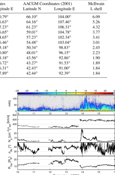
Fig. 1.LDA (15 February 14:00 UT–17 February 22:00 UT, 2004)
at the trailing edge of a fast flow. The upper panel shows the dy-namic power spectral density for THY, the next four panels the OMNI2 1-min resolution SW parameters, namely,vsw,Np,ϑBxand
Rmpfor the interval between 14–19 February 2004.
Other parameters were calculated from OMNI2 data. IMF cone angle is defined asϑBx=arccos(|Bx|/Bimf).
Magne-topause standoff distance was calculated assuming a con-stant dipolar geomagnetic field using the formula Rmp=
110.2(Npvx2)−1/6 (derived in a similar way as in Kivelson and Russell, 1995, page 172). In this formula Np, vx, and Rmp are given in cm−3, km s1, and RE, respectively.
We calculated the magnetosonic Mach number as Mms=
vsw/ q
vA2+v2
s, where vs =pγ kB(Tp+Te)/(mp+me)) is
the sonic speed,γ is the polytropic index (here = 5/3), kB is the Boltzmann constant,TpandTeare the proton and
elec-tron temperatures, mp and me are the proton and electron
masses. In this study(Tp+Te)/(mp+me)was approximated
by 2Tp/mp.
mHz
10 11 12 13 14 15 16
0 50 100
−25 −20 −15 −10 −5 0 5 10 15 20 25
400 600 800
vsw
[km/s]
10 20
Np
[cm
−3
]
30 60
ϑBx
[°]
10 11 12 13 14 15 16
10 20
September of 2004 Rmp
[R
E
]
Fig. 2. SAE (13 September 00:00 UT–08:00 UT, 2004) embedded
in a slow wind period prior to a fast solar wind stream arriving at 21:00 UT. Same format as Fig. 1.
3 Observations
3.1 Low-density anomalies and sub-Alfv´enic events
Usmanov et al. (2005) listed 23 low-density anomalies, i.e. intervals when the SW density,Np≤0.3 cm−3, and 11
sub-Alfv´enic (MA≤1) periods inferred from the OMNI2 dataset
Table 2. Low-density (Np≤0.3 cm−3) anomalies in OMNI2 data (2001–2008). Asterisks (*) indicate that a part of the hourly values is missing.
year DOY UT dur. Bimf Np vsw pdyn MA ϑBx Pc3ind
h h nT cm−3 km s−1 nPa deg. pT
2001 12 19 1 6.8 0.3 324 0.06 1.3 44 –/n.a.
2001 120 18 2 4.8 0.3 434 0.18 2.5 16 –/7∗
2001 151 11 2 6.6 0.3 360 0.10 1.4 48 9/9
2001 251 19 5 6.3 0.2 391 0.05 1.3 34 –/12∗
2001 311 7 1 8.0 0.3 651 0.38 2.2 34 11/11
2002 79 11 3 13.3 0.3 400 0.08 0.8 63 57/57∗
2002 143 22 42 10.3 0.2 589 0.12 1.1 39 8/7
2002 200 17 6 17.1 0.2 781 0.26 1.1 29 9/15
2003 187 22 2 7.1 0.3 577 0.20 2.3 46 –/18
2004 46 21 14 6.2 0.3 495 0.15 2.2 46 7/9
2004 205 2 5 13.8 0.2 633 0.16 1.0 76 –/67
2004 257 10 1 11.0 0.3 318 0.06 0.8 62 9/9
2005 20 1 4 5.4 0.3 758 0.32 4.1 63 –/30
2006 322 20 3 9.2 0.3 392 0.08 1.1 70 –/7
2006 324 14 2 7.3 0.3 323 0.07 1.2 50 7/7
Table 3.Sub-Alfv´enic (MA≤1) events in OMNI2 data (2001–2008). Asterisks (*) indicate that a part of the hourly values is missing.
year DOY UT dur. Bimf Np vsw pdyn MA ϑBx Pc3ind
h h nT cm−3 km/s nPa deg. pT
2001 170 12 1 16.0 0.6 398 0.23 1.0 52 8/8
2001 251 21 1 6.2 0.1 395 0.03 1.0 36 –/n.a.
2002 79 3 11 14.5 0.5 377 0.16 0.9 64 21/18∗
2002 144 11 24 10.1 0.1 492 0.07 0.9 48 7/7
2002 200 17 5 18.1 0.2 792 0.25 1.0 27 9/11
2003 275 5 2 18.1 1.4 302 0.24 1.0 48 8/8
2003 302 18 1 44.5 0.8 953 1.45 1.0 31 –/152
2004 205 3 1 13.9 0.2 630 0.16 1.0 72 –/31
2004 256 6 13 10.6 0.4 280 0.07 0.9 56 8/7
2006 322 21 1 9.2 0.2 390 0.06 0.9 68 –/7
condition was satisfied. The next six columns provide the averageBimf,Np,vsw,pdyn,MAandϑBx of the events. In the last column the average Pc3inds are given in pT. The val-ues separated by “/” are calculated from daylight hours/all hours data, respectively.
Usmanov et al. (2005) interpreted low-density anomalies as rarefaction of SW plasma at the trailing edge of a high speed stream from a coronal hole. We found an example (September 2004), when the SAE is connected to the lead-ing edge of a fast stream. Table 3 clearly demonstrates that sub-Alfv´enic flows are not necessarily embedded in low-density events. Sometimes a relatively high value of the IMF strength (>10−20 nT, the actual limit depends on both
vsw and Np) can also lead to a low MA, especially on 6
June 1979 (doy 157,Bimf=36 nT, event not shown in
Ta-ble 3) and on 29 October 2003 (doy 302, Bimf=44.5 nT,
vsw=953 km s−1,Np=0.8 cm−3). During the latter event,
the largest among the Halloween storms of 2003, bothBimf
andvsw had extreme values; Bimf was close to the largest
value (55.8 nT) recorded since the beginning of the space era (Veselovsky et al., 2010).
3.2 The lack of Pc3 pulsations during LDAs and SAEs
Below we present two examples of the disappearance of Pc3 (22–100 mHz) pulsations during an LDA and a SAE.
Figure 1 presents a long LDA that lasted from 15 February 2004 at 21:00 UT until 17 February 2004 at 22:00 UT. The upper panel shows the dynamic power spectrum observed at THY for the six day long interval (14–19 February 2004). The other four panels present the variation of the SW con-ditions, namely the time series ofvsw, Np, ϑBx and Rmp.
Before the LDA Np was moderately low (>2 cm−3), vsw
0 5 10 15 20 25 0
50 100 150 200
Pc3ind [pT]
THY−OMNI2 2001−2007
0 5 10 15 20 25
0 1000 2000 3000
N
p [cm −3
]
nr of cases
Fig. 3. THY Pc3 index (2001–2007) vs. proton number density
(upper panel) with 95% confidence intervals, and the histogram of
Np(lower panel).
averageRmp, whileϑBxwas highly fluctuating. Under these conditions moderate Pc3 activity was observed at THY on the ground. On 15 February, at the trailing edge of the fast wind flowNpstarted to decrease, whilevswremained high,
resulting in a highRmpby the end of the day. In the
mean-while the Pc3 ULF activity decreased but it was still observ-able. The LDA started on this day at 21:00 UT. On the fol-lowing two days, during the LDA there was no significant ULF activity in the Pc3 band. Usual ULF activity returned on 19 February. The solar wind was super-Alfv´enic during the whole event.
Figure 2 shows an example of a SAE. This event started on 12 September, 2004 at 06:00 UT and finished on 13 Septem-ber at 08:00 UT. Before and during the SAE vsw was low
(≈300 km s−1), Np dropped from low (2.5 cm−3) to
ex-tremely low (<1 cm−3),ϑBxvaried between low and moder-ately high values.Rmpincreased up to 20REduring the SAE,
and of course, the SW flow was sub-Alfv´enic. The ULF ac-tivity was low throughout the whole slow wind interval, and was the lowest during and immediately after the SAE. The situation changed on the night of 13 September when a fast wind stream with a shock front arrived, producing a pressure pulse.Rmpdecreased down to 7.5RE. On the following day
intense activity in the Pc4 band and an increased activity in the Pc3 band were observed.
In these cases the Pc3 activity is practically missing from the dayside and from the nightside, too. Similarly, Le et al. (2000a) found the magnetosphere much quieter than usual during an event in May 1999 (“the day the solar wind almost disappeared”).
These experiences, in accordance with previous ones, sug-gest that there should be a strong connection between the
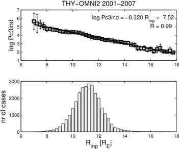
6 8 10 12 14 16 18
1 2 3 4 5 6 7
log Pc3ind
THY−OMNI2 2001−2007
log Pc3ind = −0.320 R
mp + 7.52
R = 0.99
6 8 10 12 14 16 18
0 1000 2000 3000
R
mp [RE]
nr of cases
Fig. 4. THY log Pc3 index vs. standoff distance of the
magne-topause (2001–2007). Same format as Fig. 3, but upper panel also includes the fitted curve, its equation, and the correlation coefficient of the fitted curve and the interval means.
plasma density of the SW and the ULF wave activity both in the foreshock and in the magnetosphere, as well as on the ground.
4 Statistical analysis
4.1 The role of solar wind plasma density
The SW speed control of Pc amplitudes is the most widely known relation between ground pulsation activity and the properties of the interplanetary medium, first realised by Saito (1964). The dependence of Pc3 amplitudes on Np
beside other SW parameters was also investigated by sev-eral authors (Wolfe and Meloni, 1981; Yedidia et al., 1991; Chugunova et al., 2007), but the negative correlation found was always less significant than the correlation with vsw,
e.g.R= −0.16 compared toR=0.56 observed at Pittsburgh (L=3.5) by Wolfe and Meloni (1981) in the summer of 1975, orR= −0.62 compared toR=0.86 found by Yedidia et al. (1991) based on a year-long data set of hourly aver-age integrated (Pc3 band) log power observed at L’Aquila (L=1.5) in 1985. This result was usually attributed to the fact that theNp andvsw are not independent variables,
but they themselves have a negative correlation (e.g. Hund-hausen et al., 1970; Kulcar, 1988; McComas et al., 2000; Veselovsky et al., 2010).
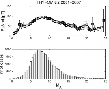
0 5 10 15 20 25 0
50 100 150
Pc3ind [pT]
THY−OMNI2 2001−2007
0 5 10 15 20 25
0 500 1000 1500 2000
M
A
nr of cases
Fig. 5. THY Pc3 index vs. Alfv´en Mach number (2001–2007).
Same format as Fig. 3.
Npis the third in importance of the eight SW parameters
in-vestigated, in spite of the fact that in itself it had practically no correlation (R= −0.16) with Pc3 activity. As an alter-native toNp the kinetic energy flux density (1/2Npmpv3sw)
yielded a relatively high correlation ofR=0.36. However, it is not clear from that work whether the inclusion ofNpin
the MLR analyses improved the correlation or not, since it was the first quantity chosen in the analysis, and the others subsequently added one by one. The maximum correlation achieved wasR=0.70 when all eight SW parameters (Np,
1/2Npmpv3sw,Bimf,Bxgsm,Bygsm,Bzgsm,ϑBx,vsw) were
in-cluded in the MLR.
Here, we demonstrate first how the THY Pc3 ampli-tudes (2001–2007 hourly means) are linked to OMNI2Np
(Fig. 3) and other Np dependent SW parameters, such as
Rmp (Fig. 4),MA (Fig. 5), Mms (Fig. 6) andpdyn (Fig. 7).
Figures 3 to 7 present these relations in the same format. In each figure the upper panel shows the dependence of Pc3ind on the chosen parameter together with the 95% confidence intervals as error bars, while in the lower panel the histogram of the occurrence frequency of the parameter considered is displayed. It can be clearly seen that all the enumerated SW parameters have some connections to ground Pc3 activity. The level of Pc3 activity dramatically drops if theNpis less than 2 cm−3(Fig. 3) or the dynamic pressure is under 2 nPa (Fig. 7), but these parameters have no or much less influ-ence above these thresholds. Pc3 activity maximises around the average Alfv´en and average magnetosonic Mach number, and rapidly vanishes toward low Mach numbers (Fig. 5 and 6). The onlyNpdependent parameter that has a significant
monotonic influence on Pc3ind in the whole value-range is the standoff distance of the magnetopause (Fig. 4); the fur-ther the magnetopause stands from the Earth, the lower the ground Pc3 activity.
0 5 10 15
0 20 40 60 80 100
Pc3ind [pT]
THY−OMNI2 2001−2007
0 5 10 15
0 1000 2000 3000 4000
M
ms
nr of cases
Fig. 6. THY Pc3 index vs. magnetosonic Mach number (2001–
2007). Same format as Fig. 3.
0 2 4 6 8 10
0 100 200 300 400
Pc3ind [pT]
THY−OMNI2 2001−2007
0 2 4 6 8 10
0 1000 2000 3000 4000
p
dyn [nPa]
nr of cases
Fig. 7. THY Pc3 index vs. dynamic pressure (2001–2007). Same
format as Fig. 3.
We note here, that except for the Np dependence itself,
which was previously noted by Ver˝o (1980) and Chugunova et al. (2007), all relationships between the Pc3 activity and theNpdependent parameters are presented here for the first
time. The presented dependences of Pc3ind onNp,Rmp,MA,
Mmsshow that any or all of them could be responsible for the
disappearance of Pc3s during LDAs and SAEs. 4.2 Separation of the influences of solar wind
parameters
0 0.1 0.2 0.3 0.4 0.5 0.6 0.7 0.8 0.9 40
60 80 100 120
Pc3ind = 51.7cos χ + 55.7 R = 0.97
Pc3ind [pT]
THY−OMNI2 2001−2007
0 0.1 0.2 0.3 0.4 0.5 0.6 0.7 0.8 0.9 0
500 1000 1500 2000 2500
cos χ
nr of cases
Fig. 8. THY Pc3 index vs. the cosine of the solar zenith angle
(2001–2007). Same format as Fig. 4.
avoid the interference of the considered parameters in our analysis, we investigated the contribution of the parameters to Pc3ind successively. The relation between Pc3ind and the parameter considered was estimated by the best-fitting poly-nomial. Then based on this relation Pc3ind was normalised to a typical value of the parameter.
In the first step the average hourly Pc3inds versus the co-sine of the solar zenith angle (χ) were binned to account for the daily variation of the Pc3 activity. The solar zenith an-gle was chosen as the first parameter, because of its obvious independence of all SW parameters. The relation between Pc3ind andχshown in Fig. 8 can be well (R=0.97) approx-imated by a linear equation. Figure 8 has the same format as Fig. 4. The linear equation was then used to normalise all Pc3ind values toχ=30◦(Pc3ind
c1).
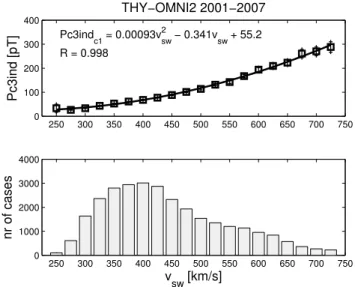
In the second step the normalised activity indices were plotted against the SW speed (Fig. 9). The resulting relation was approximated (R=0.998) by a quadratic formula. This is very similar to what is observed without normalisation (Pc3ind=0.00070vsw2 −0.248vsw+39.9pT,R=0.999); the
only significant difference is that the normalisation increased Pc3ind values by 27–30% because of our choice ofχ=30◦ as reference level in the previous step. For the second nor-malisation 400 km s−1was taken as reference level.
The dependence of the twice normalised indices (Pc3indc2) on the standoff distance of the magnetopause
(Rmp) was considered next. From the result presented in
Fig. 10 it is seen thatRmp is closely related to ground Pc3
activity and that this relation is not a simple consequence of
vsw dependence, but is an independent factor. The
depen-dence of the normalised Pc3 amplitudes onRmpcan be
mod-elled by a linear equation (R=0.98) in the 8-14 RErange.
It is different from the exponential decay found without nor-malisations (Fig. 4). For the third normalisation a reference level atRmp=10.5REwas chosen (Pc3indc3).
250 300 350 400 450 500 550 600 650 700 750 0
100 200 300 400
Pc3ind
c1 = 0.00093vsw 2
− 0.341v
sw + 55.2
R = 0.998
Pc3ind [pT]
THY−OMNI2 2001−2007
250 300 350 400 450 500 550 600 650 700 750 0
1000 2000 3000 4000
v
sw [km/s]
nr of cases
Fig. 9.Normalised (c1) THY Pc3 index vs. solar wind speed (2001–
2007). Same format as Fig. 4.
8 9 10 11 12 13 14
0 50 100 150
Pc3ind [pT]
THY−OMNI2 2001−2007
Pc3indc2 = −16.1 Rmp + 239 R = 0.98
8 9 10 11 12 13 14
0 1000 2000 3000
R
mp [RE]
nr of cases
Fig. 10. Normalised (c2) THY Pc3 index vs. standoff distance of
the magnetopause (2001–2007). Same format as Fig. 4.
0 0.1 0.2 0.3 0.4 0.5 0.6 0.7 0.8 0.9 40
60 80 100 120 140
Pc3ind
c3 = 77.4 ϑBx + 45.3
R = 0.99
Pc3ind [pT]
THY−OMNI2 2001−2007
0 0.1 0.2 0.3 0.4 0.5 0.6 0.7 0.8 0.9
0 1000 2000 3000
cos2ϑ Bx
nr of cases
Fig. 11.Normalised (c3) THY Pc3 index vs. cosine of the IMF cone
angle (2001–2007). Same format as Fig. 4.
The order of normalisation and the reference levels chosen are all arbitrary. Since three of the four parameters consid-ered here are not independent of each other, the results of the 2nd to 4th steps are determined by the particular order of steps chosen. In this section we had only one goal, to demon-strate that all the considered interdependent parameters have their own influence on ground Pc3 activity.
The analysis of partial correlations yields another ap-proach to verify the interdependence of SW parameters and to separate their influences on Pc3ind. Partial correlation, i.e. correlation between two random variables, with the effect of a set of controlling random variables removed, was computed for selected parameter pairs.
The coefficient of the anti-correlation betweenNpandvsw
was calculated at R= −0.38 for the whole period. This is consistent with the findings of Kulcar (1988), who cor-relatedvsw andNp averaged in 50 km s−1 wide SW speed
bins, and found that the correlation varied fromR= −0.36 to−0.68 during solar cycles 20 and 21, with stronger corre-lation at sunspot minima. The partial correcorre-lation ofNpand
vswafter removing the effect of the IMF strength is somewhat
stronger, i.e.R= −0.46, while the variation ofϑBx had no influence on this correlation. The anti-correlation between
vsw and Rmp was weaker (R= −0.18); however, after
re-moving the effect ofNp, it increased toR= −0.59. This was
expected, becauseRmpis a function ofvswandNp. The
cor-relation betweenNpandRmpwas even stronger,R= −0.64,
and after removing the effect ofvsw it further increased to
R= −0.77. There was no significant correlation found, how-ever, betweenϑBxand other SW parameters.
For the derivation of partial correlation coefficients be-tween Pc3ind and different parameters only dayside values (χ <90◦) were considered. The correlation coefficient be-tween Pc3ind andvswwas the highest,R=0.60. Choosing
Npas a control parameter, the partial correlation is nearly the
same,R=0.62. The correlation between Pc3ind andNpwas
rather low (R= −0.06), which explains why former authors usually did not takeNpinto account in their correlation
anal-yses. The partial correlation withvswas the control variable
is somewhat higher, R=0.24, but still does not suggest a strong connection. But if we selectRmpas control variable,
we get a more significant anti-correlation,R= −0.38, sug-gesting thatRmphas a more important role, thanNpitself.
In-deed, the anti-correlation strength between Pc3ind andRmp
isR= −0.35, which increases toR= −0.50 when removing the effect ofNp. If we use bothNpandvswas control
param-eters, the partial correlation coefficient drops toR= −0.22 meaning that the joint use ofRmpandNp in a multiple
re-gression implicitly bears a part, but not all of the information thatvswcontains.
Wolfe (1980) found that hourly mean vsw andϑBx had significant correlation (R=0.34) between 17–21 July 1975, while this behaviour ceased (R= −0.08) two weeks later (28 July–2 August), and concluded that these parameters can be considered as independent. Comparing these two time in-tervals they also found that the correlation of the log power (band integrated, 17–33 mHz, i.e. lower Pc3 range) of day-time ground pulsations observed at Pittsburgh (L=3.5) with
vswincreased (fromR=0.28 toR=0.68) between the two
intervals, while the log power –ϑBx relation remained un-changed (R= −0.40 andR= −0.38). They concluded that the higherϑBxvalues at highervswin the first interval eroded
the log power –vswrelation.
4.3 Multiple regression analysis
A MLR analysis was carried out with a carefully chosen set of variables. We started with the parameter found to have the most significant influence on the Pc3 indices, the SW speed, and added the others step by step. It was decided not to model Pc3ind by a simple linear combination of the parameters, but by the product of the parameters (pi) raised to an unknown power (αi):
Pc3ind=C·pα1 1 ·p
α2 2 ·...·p
αn
n +D, (1)
whereC andD are unknown constants. A similar formu-lation was used by Ver˝o (1980) to determine the exponent ofvsw in the expressionA=C·vswα by a simple regression
analysis. We chose this formulation for two reasons: 1. The approach based on the exponents enables one to draw con-clusions on the possible role of parameters that can be ex-pressed as the product of the investigated ones but which are not investigated directly, such as kinetic energy flux density (1/2Npmpv3sw). 2. Supposing that there is more than one
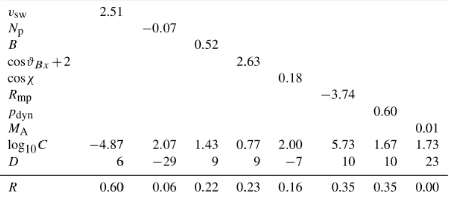
Table 4. Results of the simple regressions (Pc3ind=Cpα+D), and the correlation coefficient,R. Parametersvsw,Np,B,Rmp,pdynand
Dare in km s−1, cm−3, nT,RE, nPa and pT, respectivly.
vsw 2.51
Np −0.07
B 0.52
cosϑBx+2 2.63
cosχ 0.18
Rmp −3.74
pdyn 0.60
MA 0.01
log10C −4.87 2.07 1.43 0.77 2.00 5.73 1.67 1.73
D 6 −29 9 9 −7 10 10 23
R 0.60 0.06 0.22 0.23 0.16 0.35 0.35 0.00
be better described by the product of the controlling param-eters rather than by their sum. The sum would better fit cases where multiple independent sources are acting simul-taneously.
Equation (1) can be realised through linear regression analysis by the linear combination of the logarithms of the parameters considered:
logPc3ind=c+α1logp1+α2logp2...+αnlogpn, (2) wherecis an unknown constant. SinceCandDin Eq. (1) are constants they do not modify the correlation between the LHS and RHS of Eq. (1), henceD can be taken as zero in Eq. (2); however, bothCandDhave to be determined later for the models of Pc3ind. This can be done by a simple linear regression between Pc3ind and the MLR model (based on Eq. 2) result.
Since the logarithm is not defined for non-positive values we added 2 to the cosine of the cone angle to avoid zero as an argument when ϑBx=90◦. By choosing a value 2 we also avoided the close to zero arguments that would produce outstanding negative values distorting the result of the regres-sion analysis. Of course, 2 is an arbitrary choice, and the ac-tual value of this constant influences the resulting exponent. However, we found that the correlation coefficient does not change significantly if we increase this constant. All other parameters have positive values, including the cosine of the solar zenith angle on the dayside.
All available pulsation data recorded at Tihany between 2001–2007 and the corresponding available OMNI2 SW data together provided 28 562 samples (hourly means), which were used in these analyses to derive the presented Pc3ind models.
The results of the simple regression analyses are sum-marised in Table 4. A column of the table contains the ex-ponentαin the row of the parameterpconsidered, the con-stantsCandDfrom the equation Pc3ind=Cpα+D, and the correlation coefficientR. The different columns correspond to linear regressions for the different parameters. For
exam-ple, the first column shows that Pc3ind=10−4.87vsw2.51+6 pT, andR=0.60. This is in accordance with previous results showing that the most important factor controlling ground Pc3 activity is the SW speed. The exponent ofvswis close
to 5/2. This is in agreement with the findings of Ver˝o (1980), who found that the exponent is greater than 2 for periods less than 30 s, about 2 for periods around 30 s, and less for longer periods.
Again in accordance with previous studies (e.g. Ver˝o, 1980; Chugunova et al., 2007) there is no correlation be-tweenNp and Pc3 activity (Table 4, second column). This is shown both by the low correlation coefficient and the close to zero exponent. Although it was demonstrated that in the lowest range of values (Np<2 cm−3)Npdoes have a strong
effect on Pc3ind (Fig. 3), there is no dependence above this threshold. The situation is similar forMA(Fig. 5), where we
can find correlation in some intervals, but when the whole range of possible values are taken into account, the corre-lation coefficient is close to zero. On the other handϑBx,
Bimf, Rmp and pdyn all seems to have some influence on
Pc3ind (Table 4). The correlation in the case ofRmpis an
anti-correlation as shown by the negative exponent.
Tables 5 to 7 present the results of MLRs in a similar way to Table 4. The columns of Table 5 contain the expo-nents of the best fittingCvα1
swpαi2+Dmodels, wherepi=Np,
B, etc., and the correlations between models and observa-tions. For example, the first column presents a model in which log10C= −7.30, D=14 pT, α1=3.28, α2=0.48,
andR=0.65. Each column is an independent MLR model. Table 5 includes MLRs usingvsw, which was previously
found to be the most important parameter (Table 4), and an-other parameter. The inclusion ofNp, or any of the other
density related parameters,Rmpandpdyn, pushes up the
cor-relation coefficient equally to R=0.65, while ϑBx andχ have somewhat lower influence. The inclusion of other pa-rameters hardly modifies the result.
We choseNpas the second parameter. Hence in the MLRs,
Table 5.Results of the 2-D MLRs (Pc3ind=Cvα1
swp2α2+D), and the correlation coefficient,R.
vsw 3.28 2.39 2.44 2.51 2.31 2.33 2.55
Np 0.49
B 0.27
cosϑBx+2 2.32
cosχ 0.18
Rmp -2.92
pdyn 0.48
MA 0.17
log10C −7.30 −4.77 −5.63 −4.79 −1.34 −4.60 −5.14
D 14 8 6 5 14 15 6
R 0.65 0.61 0.64 0.63 0.65 0.65 0.61
Table 6. Results of the 3-D MLRs (Pc3ind=Cvα1
swNpα2pα33+D), and the correlation coefficient,R.
vsw 3.26 3.35 3.30 2.09 3.37 3.28
Np 0.48 0.58 0.49 −0.11 0.53 0.49
B 0.02
cosϑBx+2 2.92
cosχ 0.19
Rmp −3.57
pdyn −0.05
MA −0.02
log10C −7.28 −8.70 −7.25 −0.01 −7.57 −7.30
D 15 12 12 14 14 15
R 0.65 0.71 0.68 0.65 0.65 0.65
parameter were used to model Pc3ind. Here theϑBx as a third parameter produced the highest increase in correlation, then cosχfollows with an exponent∼1/5, while neitherRmp,
norpdynis able to further increase the strength of the
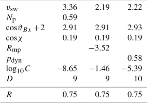
corre-lation. The correlation coefficient, however, can be increased further (up toR=0.75) by adding both the cone angle and the solar zenith angle to the parameter set (Table 7).
Similar results to Table 6 can be achieved if we replaceNp
by eitherRmp orpdyn (not shown). In each MLR both the
exponent of the third parameter and the correlation strength are very close (within 0.03 and 0.01) to their corresponding values in Table 6. In terms of the MLR model the three den-sity related parameters are interchangeable. For comparison, Table 7 presents the MLR models in whichvsw,ϑBx, one of the three density related parameters, and a fourth parameter resulting in the highest correlation were considered. The ex-ponent ofvswis different in the different columns, because
of its close relation toNp,Rmpandpdyn. The choice of the
density related parameter, however, did not influence the ex-ponents ofϑBx significantly. In each caseχ was found as the fourth most important parameter with the same exponent. Furthermore, the strength of the correlations are the same.
MLRs were also executed separately for each year (Ta-ble 8). The results for both the correlation coefficients
Table 7.Results of the 4-D MLRs (Pc3ind=Cvα1
swpα22(cosϑBx+ 2)α3cosα4χ+D, wherep
2=NporRmporpdyn), and the correla-tion coefficient,R.
vsw 3.36 2.19 2.22
Np 0.59
cosϑBx+2 2.91 2.91 2.93
cosχ 0.19 0.19 0.19
Rmp −3.52
pdyn 0.58
log10C −8.65 −1.46 −5.39
D 9 9 10
R 0.75 0.75 0.75
and the exponents are similar. The exponents ofvsw, Np,
cosϑBx+2,cosχ are about 3, 3/5, 3, 1/5, respectively. In the four parameter MLRs the exponents of Rmp andpdyn
were found to be around−3 and 1/2 (not shown).
During the period investigated the maximum to minimum ratio of the observed values ofvsw,Np,Rmpandpdynwere
4.6, 790, 3.5 and 1702, respectively. However, when deter-mined from the above exponents these ratios change to 97, 55, 43 and 41, characterising the importance of the param-eters in the explanation of the variability of the Pc3 index. This result underlines again the priority ofvsw, and shows
thatNp,Rmpandpdynare about equally important.
In Table 9 the results of four parameters MLRs for other stations are presented (only 2003 data were used). Based on these findings it can be stated that most of the above con-clusions are valid also at higher latitudes. There are some differences, however. The role ofχand evenϑBx decreases with increasing latitude (decreasing exponent) and, more im-portantly, the correlation coefficient clearly decreases. 4.4 Artificial Neural Networks
Table 8.The results of the 4-D MLRs for different years (Pc3ind=Cvα1
swNpα2(cosϑBx+2)α3cosα4χ+D).
THY 2001 2002 2003 2004 2005 2006 2007
vsw 2.88 3.20 3.26 3.23 2.48 3.53 3.50
Np 0.57 0.62 0.63 0.60 0.47 0.56 0.56
cosϑBx+2 2.99 2.93 3.07 3.21 2.31 2.98 2.66
cosχ 0.23 0.23 0.21 0.17 0.16 0.15 0.14
log10C −7.34 −8.17 −8.37 −8.41 −5.85 −9.12 −8.92
D 1 5 4 6 7 1 −2
R 0.71 0.74 0.76 0.75 0.69 0.76 0.80
Table 9.The results of the 4-D MLRs, 2003, MM100 stations (Pc3ind=Cvα1
swNpα2(cosϑBx+2)α3cosα4χ+D).
2003 THY BEL TAR NUR HAN SOD KIL
vsw 3.26 2.08 2.66 2.85 2.86 2.49 2.70
Np 0.63 0.27 0.48 0.54 0.54 0.46 0.50
cosϑBx+2 3.07 2.29 2.27 2.35 2.32 1.66 1.56
cosχ 0.21 0.22 0.18 0.14 0.11 0.06 0.04
log10C −8.38 −4.22 −6.16 −6.68 −6.73 −5.34 −5.94
D 4 −31 −6 1 2 59 93
R 0.76 0.75 0.65 0.65 0.65 0.46 0.45
networks (ANN’s) with various sets of input parameters, similar to those used in the development of the MLR model, to find a set of inputs that optimally model the output param-eter, Pc3ind.
Since the use of ANN’s is not common in Pc3 studies, we offer a short description of neural networks. For an extensive exploration of the subject, the reader is referred to dedicated texts (e.g. Haykin, 1999; Fausett, 1994; Bishop, 1995).
Artificial neural networks are parallel computational struc-tures, represented by a weighted network of computational nodes, capable of performing complex (non-linear) regres-sion and classification tasks (Haykin, 1999). In this case we use the ANN as a regression model to approximate the output parameter Pc3ind, using a set of input parameters. Multilayer feedforward neural networks (Haykin, 1999), the type we are using, consists of three types of computational nodes: in-put nodes (comprising the inin-put layer), hidden nodes (which can be collected in multiple hidden layers) and output nodes forming the output layer.
Such an ANN withN input nodes,M hidden nodes in a single hidden layer, and one output node, may be represented by Eqs. (3) and (4) (Bishop, 1995, for example):
Hj =fH N X
i=1 h
w(i,j1)Ii i
!
, j∈ {1, ... , M} (3)
O=fO
M X
j=1 h
wj(2)Hj i
!
(4)
Input nodesIi are the independent variables and their values are simply the respective sets of input parameter measure-ments. Hidden nodesHj apply an activation function fH,
usually sigmoidal, and tanh in our case, to the sum of the in-put parameter values, weighted bywi,j(1). The number of hid-den nodes and layers determine the network’s ability to re-solve highly non-linear behaviour, and are determined by the modeller (Haykin, 1999). The output node computes the ap-proximation to the modelled system by applying a linear acti-vationfOto the sum of the hidden node outputs, weighted by
w(j,k2). The output approximating Pc3ind is thus determined by the network as a function of the input parameters and the weights.
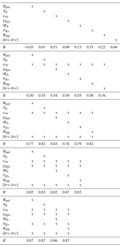
Table 10. Evolution of the wrapper process. Inputs are iteratively added (denoted by x’s) according to the performance of the associated network. The set of inputs yielding the highest correlation between measured and modelled output (R) are kept, and the rest of the candidate inputs are varied in the next round of training. Also see Fig. 12.
Bimf x
Np x
vsw x
pdyn x
MA x
ϑBx x
Rmp x
[hrs,hrc] x
R −0.03 0.01 0.51 0.09 0.15 0.35 0.22 0.46
Bimf x
Np x
vsw x x x x x x x
pdyn x
MA x
ϑBx x
Rmp x
[hrs,hrc] x
R 0.50 0.55 0.54 0.50 0.55 0.56 0.76
Bimf x
Np x
vsw x x x x x x
pdyn x
MA x
ϑBx x
Rmp x
[hrs,hrc] x x x x x x
R 0.77 0.82 0.83 0.76 0.79 0.82
Bimf x
Np x
vsw x x x x x
pdyn x x x x x
MA x
ϑBx x
Rmp x
[hrs,hrc] x x x x x
R 0.82 0.83 0.82 0.87 0.83
Bimf x
Np x
vsw x x x x
pdyn x x x x
MA x
ϑBx x x x x
Rmp x
[hrs,hrc] x x x x
We set up many ANN’s with various sets of input pa-rameters, and evaluate each network, to find a set of in-put parameters that optimally reproduce the target data set (Sect. 4.4.1). Seven solar wind- and IMF-based parameters are identified, along with two time-based parameters. The sine and cosine of UT hour of the day,hrs=sin224π·hour andhrc=cos224π·hour, are included in the set of candi-dates to model the diurnal variation in Pc3 activity. Employ-ing this pair as input parameters to an ANN is equivalent to using the linear combinationα hrs+β hrcas a single input, where the coefficients α andβ are just the weights deter-mined by the network training algorithm (see Eq. 3). During training the weights are adapted to optimally reproduce the periodic component of the output parameter. Note that we usehrsandhrctogether as a pair of input parameters, since the sine-cosine pair is needed to resolve the periodic compo-nent of the output (i.e. so that hour 1 follows after hour 24). The solar wind- and IMF-based candidate input parameters considered are: solar wind speedvsw, cone angleϑBx, IMF magnitudeBimf, solar wind plasma densityNp, the dynamic
pressure,pdyn, the magnetopause standoff distanceRmp, and
the Alfv´enic Mach numberMA.
The training set consists of data collected for 2003 (from day 1 to day 365), while the testing data set covers the inter-val from hour number 1800 to hour number 2500 of 2002, corresponding to about 29 days.
The testing and training sets are reduced by excluding in-stances where the planetaryKindex is above 4. This mea-sure is taken to enmea-sure that geomagnetic storm activity is not included in this model. The result is a training data set of 6551 values per parameter (out of a possible 8760 h in the year), while the length of the testing set is 639 (out of 700). 4.4.1 Wrapper process
We employ an ANN wrapper to find the subset of candidate input parameters bearing most influence on the output pa-rameter. A “wrapper” refers to a model dependent feature selection process whereby many models are evaluated and the best performing one selected (e.g. Kim et al., 2005).
Our wrapper is implemented by training and evaluating many ANN’s, each with similar configuration, but a different set of input parameters for each network. Every network is trained and evaluated on the data sets described in the pre-vious section. The simulation procedure commences with the training and testing ofmANN’s each with a single in-put parameter (m=8 in this case). Theminput parameters are ranked according to each corresponding network’s per-formance. The input parameter corresponding to the best-performing ANN is kept, while the remainingm−1 param-eters are varied to formm−1 pairs of input parameters to be used in the next round of training. The process con-cludes when all parameters are included as inputs or when the change in network performance due to adding another
1 9 16 22 27 30
−0.1 0 0.1 0.2 0.3 0.4 0.5 0.6 0.7 0.8 0.9
Network #
Correlation (measured vs. modeled)
1 Input 2 Inputs 3 Inputs 4 Inputs Inputs5 Vsw, [hrs, hrc]
Vsw
Vsw, [hrs, hrc], Pdyn, θ Bx Vsw, [hrs, hrc], Pdyn
Fig. 12.Correlation between measured and modelled Pc3ind as
in-puts are added according to the wrapper process. Vertical dashed lines indicate the start of a new round of training. Red squares de-note the winner of each round of training, with the corresponding input parameters displayed. See Table 10 for a detailed illustration of the process.
input parameter stabilises, such that an unambiguous choice is not possible.
The wrapper process is summarised in Table 10 and il-lustrated in Fig. 12. Each network is trained using the in-put parameters marked by x’s. The resulting correlation be-tween measured and predicted output is listed in the last row. Figure 12 plots the model performance (correlation between measured and predicted output), versus network trained, as input parameters are varied and added according to the wrap-per process. The wrap-performance due to each new addition to the optimal set is indicated, and the updated set of inputs listed accordingly. After each round of training a new in-put is added to the set of influential inin-puts. After the first round of training, the SW speed emerges as the most influen-tial input for single-input networks. Note that in the wrapper process we treat the time-based pair [hrs, hrc] as a single parameter. The correlation between measured and predicted validation data isR=0.51 forvsw. Time [hrs,hrc] andϑBx also yields significant correlation between measured and pre-dicted Pc3ind atR=0.46 andR=0.35, respectively.
In the second round of training, pairs of inputs –vswand
another input from the set of candidates – are used for each network. All pairs of inputs yields prediction accuracy of at least R=0.5. The optimal pair of inputs are the [hrs,
hrc] pair and andvsw yieldingR=0.76 correlation between
measured and predicted output. Other parameters add less to the accuracy of the prediction achieved in the first round – thevsw,ϑBxpair withR=0.55 andvsw,RmpwithR=0.56,
03/29 03/30 03/31 04/01 04/02 04/03 04/04 04/05 0
100 200 300 400 500 600
Time [mm/dd] (2002)
Pc3Ind [pT]
Measured MLR ANN
RMLR = 0.86 Input: vsw, χ, pdyn, ϑBx
R ANN = 0.87
Input: vsw, [hrs,hrc], pdyn, ϑBx
Fig. 13. Measured (solid curve) and modelled (red for ANN and
green for MLR model) Pc3ind for a week included in the testing data set, using the optimal set of input parameters as indicated. The correlation between measured and modelled outputs are 0.87 for the ANN and 0.86 for the MLR model.
R=0.83 correlation;(ii)vsw, [hrs,hrc],RmpatR=0.82;
and(iii)vsw, [hrs,hrc],NpatR=0.82 correlation between
measured and predicted Pc3ind. The two best-performing candidates,pdynandRmp, are both directly related to the size
of the magnetosphere and the density,Np (along withvsw),
defines the dynamic pressure. Although the choice is some-what ambiguous on account of the close separation in corre-lation coefficients, we selectpdynand continue with the
pro-cess. The similarity of these three parameters is further illus-trated by the correlation between them: calculating the cor-relation coefficient between the pairspdyn,Npandpdyn,Rmp
over the testing data set yieldsR=0.88 andR= −0.78, re-spectively. The ANN models are sensitive to this fact, given that subsequent rounds of training do not yieldRmp or Np
as important – as they do not add any new information to a model withpdyn already included in the set of inputs. As is
the case with the MLR models, any one ofRmp,Nporpdyn
could be included at this stage.
We conclude the wrapper process after four rounds of training – withvsw, [hrs, hrc], pdyn andϑBx as the final set of influential inputs. The correlation between measured and predicted Pc3ind at this stage isR=0.87. The other sets of inputs all yield accuracy of approximatelyR=0.82 and do not improve on the previous round’s result. A fifth round of training is performed, but no new input is added to the set as no improvement upon the previous round of training is made (see Table 10 and Fig. 12, networks 27 to 30). We conclude that the remaining candidate inputs do not add any new information to the model.
4.4.2 Comparison of MLR and ANN wrapper results
The ANN modelling procedure yields four parameters,
vsw,[hrs, hrc], pdyn, ϑBx
as the most influential subset of inputs from the candidates. We recall here, thatpdynis interchangeable withNporRmp;
the ANN does not prefer one above the others. After four rounds of training, the increase in network performance due to the addition of input parameters is negligible and no fur-ther inputs are added.
This result is in agreement with previous studies not-ing the correlation between vsw, ϑBx and Pc3 amplitude (e.g. Saito, 1964; Bol’shakova and Troitskaya, 1968; Wolfe, 1980). Furthermore, we know that Pc3 are a largely dayside phenomenon, hence the strong dependence of Pc3ind on the hour of the day. This result is also in accordance with our results based on MLR analysis. Both methods resulted in a four parameter model, in which the density related parameter can be any ofpdyn,Rmp, orNp.
However, the ANN and MLR results cannot be compared directly. In the MLR analysis we used only dayside data, while in the ANN approach both day and night data were utilised. For the sake of a closer comparison we recalculated the 2003 MLR results for THY including night data. We took firstvswas a model parameter, then added cosχ,pdyn
and cosϑBx step by step. The correlation increased grad-ually, and wasR=0.42, 0.69, 0.72 and 0.81, respectively. Note, that we added 2 to cosχand cosϑBx to avoid zero and negative values whenχ >=90◦(nightside) orϑ
Bx=90◦, so that log of cos can be taken.
Applying the MLR models inferred from 2003 observa-tions for the test period of ANN (17 March–15 April 2002), the correlation was even higher, R=0.49, 0.76, 0.81 and 0.86, for the different parameter sets, respectively, very close to the ANN correlation values (R=0.51, 0.76, 0.83 and 0.87). Although ANN, as expected, yields a slightly more accurate result, MLR has the advantage that it yields an an-alytical model. For example, Eq. (5) is the aforementioned four parameter MLR model (based on Eq. 2) obtained from 2003 data as described in Sect. 4.3:
Pc3ind[pT] =4.064·10−5vsw1.650·(cosχ+2)1.946
·p0dyn.540·(cosϑBx+2)2.675−16 pT, (5) wherevswis in km s−1, andpdyn in nPa. A comparison of
100 200
Pc3Ind [pT]
400 800
Vsw
[km/s]
45 90
ϑBx
[
°
]
144.00 144.12 145.00 145.12 146.00 146.12 0
1 2
P [nPa]
0 2 4
UT [doy.hh]
Np
[#/cm
3]
Measured ANN MLR
Fig. 14.Measured (solid) and modelled (dotted) Pc3ind during an
LDA over 24–26 May 2002 (top panel), along with SW speed (2nd panel), cone angle (3rd panel), and SW dynamic pressure (solid curve, left axis) and plasma density (dotted curve, right axis) in the bottom panel.
4.4.3 Testing the ANN model prediction during low-density events
An LDA on 24–25 May 2002 yielded very low pressure (pdyn<0.4 nPa) and particle count (Np<0.3cm−3) in the
SW plasma for most of the 48 h period. Starting from 11:00 UT on 24 May, the solar wind became sub-Alfv´enic. In this section we test the MLR (Eq. 5) and ANN (developed in Sect. 4.4.1) models during this LDA event. Input parame-ter measurements from 24 to 26 May 2002 are used to predict Pc3ind, using both models. Measured Pc3ind is close to zero on 24 and 25 May, with weak activity on the third day.
Figure 14 illustrates the essence of what is described in this section: The top panel of Fig. 14 shows the measured (blue curve) and modelled (MLR – green, ANN – red) Pc3ind for 24–26 May 2002, measured at THY. In the second and third panelsvswandϑBx from OMNI2 are plotted for the same period, respectively. The bottom panel of Fig. 14 depicts the SW dynamic pressure (solid blue line, left-hand axis) and plasma density (dotted red line, right-hand axis) during the interval, also from the OMNI2 set.
On 24 May both models predict moderate pulsation ac-tivity – peaking near 90 pT (MLR; Fig. 14, top panel, green curve) and 190 pT (ANN; Fig. 14, top panel, red curve), re-spectively. Both models appear to react to favourable SW conditions, withvsw>600 km s−1andϑBx<50◦. However, the measured activity (Fig. 14, top panel, blue curve) is very weak at a constant near-zero rate for the entire day along with a very low pressure (bottom panel, blue curve) and density (bottom panel, red curve).
On 25 May SW speed (Fig. 14, second panel) and cone angle (third panel) conditions are less favourable, with the speed decreasing to around 400 km/s and the cone angle in-creasing to above 50◦. The plasma density and dynamic
pres-sure continues at very low levels (below 0.5 particles/cm3 and 0.5 nPa, respectively). In this case the models react well to the combination of unfavourable speed, IMF direction, and pressure conditions, predicting very low (Pc3ind <30 pT) activity.
On 26 May some activity is observed (Fig. 14, top panel, blue curve). Solar wind speed remains average, around 400 km s−1and the cone angle above 40◦. The density (pres-sure) increases step-like from around 0.5 cm−3(0.1 nPa) to approximately 3cm−3(2 nPa) after 18:00 UT on 25 May, re-maining near this level for the entire day. In this case both the ANN (red curve) and MLR (green curve) models accu-rately predict the observed activity – apparently reacting to the increase in pressure, in addition to moderatevswandϑBx conditions.
Both the ANN and MLR models are sensitive tovswand
ϑBxconditions (24–26 May) and to the combination ofvsw,
ϑBx andpdyn (25–26 May); however on 24 May, the
com-bination of high SW speed and small cone angle dominates the low pressure and the models incorrectly predict moder-ate pulsation activity. The insensitivity of the models to ex-tremely low pressure is due to the relative rarity of LDA’s with respect to more normal pressure and density conditions in the solar wind. In order for an ANN to correctly model a certain aspect of the modelled system, it must be adequately represented in the training set of data. The fraction of train-ing data set measurements withpdyn <1.0 nPa is 9.8% and
only 2% of the data haspdyn <0.5 nPa. The modelling of
low-density events could hence be improved increasing the fraction of low-density data in the training set.
5 Discussion
During most of the LDAs and SAEs listed in Tables 2 and 3 the level of Pc3 activity was extremely low (Pc3ind <
10−20 pT, given in the last columns of the tables), and close to the noise level of the instrument (6–7 pT rms in the Pc3 band) which does not coincide with unusually low SW speed or high cone angle. In 6 of 8 LDA events for which day-side Pc3ind values observed at THY were available, ϑBx was not more than 50◦, and in all cases less than 65◦. The same ratios for SAEs were 3 of 6 and 6 of 6. Similarly,
vsw was higher than 300 km s1during all LDAs and during
5 of 6 SAEs for which dayside Pc3 data were available, and higher than 450 km s−1for half of the LDAs and 1/3 of the SAEs. These solar wind conditions are not unfavourable, and in some cases decidedly favourable for UW generation.
Le et al. (2000a) found that during the LDA+SAE of May 1999 Pc3s were absent, although the IMF cone angle was favourable (∼40◦) for UW generation, andvswwas
moder-ately low (350 km s−1).
During LDAs the magnetosphere calms and the upstream interplanetary region may become quiet. E.g. during the May 1999 LDA event Smith et al. (2001) and Le et al. (2000a) reported one order of magnitude decrease of the ULF wave activity in the ion-foreshock. During the rarefaction inter-val, the rms ofBimf underwent a factor of 5–10 reduction
(0.1–0.2 nT) compared to the fluctuations in the neighbour-ing plasma (1 nT). Smith et al. (2001) explained this be-haviour by the refraction of fast-mode ULF waves away from the regions where the Alfv´en speed is high. We prefer an al-ternative explanation, that is, since there were practically no protons present in the foreshock the generation of upstream ULF waves through wave-particle interaction would be much weaker. Le et al. (2000a) raised the idea that extremely low Mach number (Mms) could be responsible for the pause in
ULF activity in May 1999. They supposed that the low Mach number shock reflected very few particles. They also empha-sised that a potential effect of the Mach number should be separated from the dependence of the activity onvsw.
We demonstrated by statistical analysis that beside vsw
andϑBx,Npor another solar wind density related
parame-ter also has a key role in the control of dayside Pc3 activ-ity. Both MLR and ANN analyses rankedNpmore
impor-tant thanϑBx. Earlier works have already raised the possibil-ity thatNpmay play some role, however, its influence from
other SW parameters had not yet been separated. A similar strong dependence in the low-density range was also found by Ver˝o (1980) atL=1.9 in the 50–200 mHz band whenever
Npwas lower than 5 cm−3(the lowest bin used in that study
was 0−5 cm−3) and by Chugunova et al. (2007) in the Pc3 band at auroral and near-pole latitudes (forNp<2 cm−3).
At higher Np values the Pc3 amplitudes slowly decreased
with increasing SW density. This tendency can be clearly ob-served in our results (Fig. 3), as well. Ver˝o (1980) also found that the Np dependence was strong in the same frequency
bands where the implicitvswdependence suggests that this
relation is just a consequence of the interdependence of these parameters. Wolfe and Meloni (1981) realised that aftervsw
andϑBx,Npis the third parameter that has a significant effect
on ground (17–33 mHz) pulsations atL=3.5. All of these results imply thatNphas a similar role at low, medium and
high latitudes, thus suggesting a common source of dayside Pc3s over large regions. However, none of the cited authors interpreted their results in depth.
To our knowledge the dependence of Pc3 activity on other density related parameters, except for flux density and dy-namic pressure has not been investigated. Here we demon-strated a relationship with the Alfv´enic and magnetosonic Mach number, with the SW dynamic pressure, and with the standoff distance of the magnetopause. We also showed that
Np,pdynandRmpare equally important and interchangeable
parameters in MLR and ANN empirical models. In the fol-lowing we give a physical interpretation of the found rela-tions.
There are several possibilities of howNp may affect
sur-face Pc3 activity:
1. In the absence of upstream protons, ULF waves cannot be generated. Upstream ULF waves gain their energy from back scattered SW particles via the ion-cyclotron mechanism (e.g. Gary, 1978; Yumoto et al., 1984; Le and Russell, 1994; Heilig et al., 2007b). Fewer particles mean less energy to be transferred during wave-particle interactions. This may be one of the reasons why there are no Pc3s whenNpis extremely low (<2 cm−3). It
would appear that the SW proton density acts as an “on-off” switch for mid-latitude dayside Pc3s, in the sense that under moderateNpthe Pc3 amplitude is governed
mostly by the SW speed, IMF direction (ϑBx) and lo-cal time as on 26 May (Fig. 14). However, under very low proton counts (24, 25 May), Pc3 activity disappears regardless of otherwise favourable SW plasma condi-tions. This agrees with data in Fig. 3, where Pc3 activity ceases for number densities below 2 cm−3, while above this threshold, the density only weakly influences Pc3 amplitude.
2. WhenNpis low the bow shock may become weak (i.e.
MAis low), hence the protons are reflected back less
ef-ficiently (Thomsen et al., 1993; Kucharek et al., 2004), which can lead to the decrease of upstream ULF wave activity (Le et al., 2000a). Onsager et al. (1990) and Thomsen et al. (1993) found that there is a definite ten-dency for the beams of near-specular reflected ions to be absent at the lower (<5) Mach numbers. Without reflected ions, upstream waves will not be generated. 3. As the SW flow becomes sub-Alfv´enic (MA<1),
up-stream ULF waves that are propagating upup-stream at the Alfv´en speed in the plasma frame (Yumoto et al., 1984; Narita et al., 2004; Heilig et al., 2007b) are not effi-ciently convected back downstream toward the shock, and cannot enter the magnetosphere. Thus UWs are not able to act as a source of ground Pc3 activity under sub-Alfv´enic conditions.
4. Low plasma density results in larger standoff distance of the bow shock and the magnetopause nose, i.e. the ULF waves have to propagate over a longer path to reach the ionosphere and the ground. If there is some kind of damping present in the magnetosphere it could explain the observed amplitude reduction. During the famous 1999 event the Earth’s bow shock was crossed by the Wind spacecraft as far as 53REin radial distance from
without damping. Therefore, in the MHD frame one can only count on geometric effects, e.g. the exponential decay of the evanescent mode (Takahashi et al., 1994). Compressional mode waves can propagate in any direc-tion. Supposing a point-like source (e.g. the subsolar point of the magnetopause) and spherical wave fronts compressional waves will suffer attenuation with a fac-tor of 1/r, whereris the distance from the source, as a consequence of spatial spreading of the wave front. This type of attenuation is called geometric attenuation. We found, however, a much stronger exponential de-cay as shown in Fig. 4. The attenuation can be given in the form Pc3ind=Pc3ind0e−λr, where Pc3ind0 is
the the amplitude index at r0=1RE. In the case of
THY the apparent attenuation factorλis 0.32, mean-ing that 50% ((e−0.32)2≈0.53) of the wave energy is lost atdr=1REdistance. The real attenuation can be
smaller, since as we showed in Fig. 10, after we had nor-malised Pc3ind withvswthe attenuation became close to
linear, decreasing Pc3ind with 16 pT atdr=1RE
dis-tance. Further studies and multipoint observations in the magnetosphere are needed to find the real attenuation factor, its location, and the physical processes responsi-ble.
Although all four of the scenarios described above are pos-sible and can be responpos-sible for the disappearance of Pc3s during LDAs, none of them has been discussed in detail or verified using empirical data prior to this study.
We also derived empirical models that can be used to pre-dict Pc3 amplitudes at any local time. The model parameters for THY and other MM100 stations are given in Tables 7, 8 and 9. In spite of the obvious SW density dependence in-corporated in the models it cannot account for the disappear-ance of Pc3s at LDAs and SAEs as was shown in Sect. 4.4.3. The reason for this may be that there is more than one mech-anism at work, simultaneously. Mechmech-anism 2 is supported by direct foreshock observation of the decrease of wave en-ergy during a SAE (Le et al., 2000a). However, we think that mechanism 1 can also be responsible. More foreshock observations are needed to discriminate between these pos-sibilities. Mechanism 3 should also act as a switch for UW related Pc3 activity according to UW theory. Mechanism 4, the attenuation of ULF wave energy with distance, should act continuously and we think that this phenomenon is the source of the sensitivity of our models on the variation ofNp. This
is the only mechanism of the four that has a strong effect over the range of measurements observed. Mechanisms 1, 2 and 3 seem to be important under conditions of extremely lowNp.
We found that the roles ofχandϑBxin controlling Pc3ind to decrease with increasing latitude as can be concluded from the decreasing correlations seen in Table 9. It implies that mid latitude (L=1.8−3.8) Pc3 activity is more tightly linked to the UWs than that at higher latitudes. This fact can be a result of a low latitude (e.g. subsolar) source, but it can
also mean that there are other dayside Pc3 sources at higher latitudes not controlled or controlled but in a different way by the considered parameters.
The upstream wave source mechanism is only one of the ways the solar wind can drive dayside magnetospheric ULF waves. The decelerated solar wind plasma flowing in the magnetosheath may generate surface waves on the flanks of the magnetopause via the Kelvin-Helmholtz instability. Kelvin-Helmholtz waves which have a typical time scale of a few minutes (i.e. in the Pc4-Pc5 band) in turn may couple to internal resonances inside the magnetopause as realized first in the 1970s by Southwood (1974); Chen and Hasegawa (1974). As a consequence of the generation mechanism, Kelvin-Helmholtz waves are more intense at high SW speeds (similar to UW generated Pc3’s), but also have a dawn and a dusk peak in the local time distribution of their power, unlike the power of UW generated Pc3’s, that peaks around local noon.
The SW dynamic pressure fluctuations (and frozen-in magnetic field) can also be a source of dayside compressional ULF waves. Kepko et al. (2002) have shown that ULF waves at discrete frequencies (0.4–3 mHz) are sometimes directly driven by density oscillations present in the undisturbed am-bient solar wind.
Pressure pulses in the solar wind may cause impul-sive compressions of the magnetosphere, capable of excit-ing broad band compressional waves in the magnetosphere which can couple to cavity (Kivelson and Southwood, 1985; Lee and Lysak, 1989) or waveguide (Samson and Rankin, 1994) modes. We should note, however, that observational evidence for global fast mode cavity resonance or waveguide mode is still very limited (Samson and Rankin, 1994; Waters et al., 2002).
Beside these external sources, internal disturbances can also lead to wave generation. E.g. irregularly shaped 7– 25 mHz waves referred to as Pi2s are clearly linked to sub-storm activity (e.g. Saito et al., 1976).
Pc3–Pc5 pulsations can be observed everywhere in the magnetosphere, generally as a superposition of externally or internally driven waves and the resonant response of the mag-netosphere. Previous works (e.g. Ver˝o, 1980; Wolfe and Mel-oni, 1981; Wolfe et al., 1985; Chugunova et al., 2007) have demonstrated that although under strong SW control, Pc3, Pc4 and Pc5 pulsations react differently to changes in SW conditions, possibly due to their different origins. Pc2s (100– 200 mHz) are very rarely observed at mid latitudes (Saito, 1969; Anderson et al., 1992). Thus, although the band of UWs covers also the higher part of the Pc4 range, we re-stricted our study to Pc3s, to avoid unnecessary mixing of physical phenomena which could have “contaminated” our result.