www.atmos-chem-phys.net/16/1003/2016/ doi:10.5194/acp-16-1003-2016
© Author(s) 2016. CC Attribution 3.0 License.
The impacts of aerosol loading, composition, and water uptake on
aerosol extinction variability in the Baltimore–Washington,
D.C. region
A. J. Beyersdorf1, L. D. Ziemba1, G. Chen1, C. A. Corr1,2, J. H. Crawford1, G. S. Diskin1, R. H. Moore1, K. L. Thornhill1,3, E. L. Winstead1,3, and B. E. Anderson1
1NASA Langley Research Center, Hampton, Virginia, USA 2Oak Ridge Associated Universities, Oak Ridge, Tennessee, USA 3Science Systems and Applications, Inc., Hampton, Virginia, USA
Correspondence to:A. J. Beyersdorf ([email protected])
Received: 5 August 2015 – Published in Atmos. Chem. Phys. Discuss.: 28 August 2015 Revised: 16 November 2015 – Accepted: 21 December 2015 – Published: 28 January 2016
Abstract.In order to utilize satellite-based aerosol measure-ments for the determination of air quality, the relationship between aerosol optical properties (wavelength-dependent, column-integrated extinction measured by satellites) and mass measurements of aerosol loading (PM2.5 used for air
quality monitoring) must be understood. This connection varies with many factors including those specific to the aerosol type – such as composition, size, and hygroscopicity – and to the surrounding atmosphere, such as temperature, relative humidity (RH), and altitude, all of which can vary spatially and temporally. During the DISCOVER-AQ (De-riving Information on Surface conditions from Column and Vertically Resolved Observations Relevant to Air Quality) project, extensive in situ atmospheric profiling in the Balti-more, MD–Washington, D.C. region was performed during 14 flights in July 2011. Identical flight plans and profile lo-cations throughout the project provide meaningful statistics for determining the variability in and correlations between aerosol loading, composition, optical properties, and meteo-rological conditions.
Measured water-soluble aerosol mass was composed pri-marily of ammonium sulfate (campaign average of 32 %) and organics (57 %). A distinct difference in composition was ob-served, with high-loading days having a proportionally larger percentage of sulfate due to transport from the Ohio River Valley. This composition shift caused a change in the aerosol water-uptake potential (hygroscopicity) such that higher rel-ative contributions of inorganics increased the bulk aerosol
hygroscopicity. These days also tended to have higher rel-ative humidity, causing an increase in the water content of the aerosol. Conversely, low-aerosol-loading days had lower sulfate and higher black carbon contributions, causing lower single-scattering albedos (SSAs). The average black carbon concentrations were 240 ng m−3in the lowest 1 km,
decreas-ing to 35 ng m−3in the free troposphere (above 3 km).
Routine airborne sampling over six locations was used to evaluate the relative contributions of aerosol loading, compo-sition, and relative humidity (the amount of water available for uptake onto aerosols) to variability in mixed-layer aerosol extinction. Aerosol loading (dry extinction) was found to be the predominant source, accounting for 88 % on aver-age of the measured spatial variability in ambient extinc-tion, with lesser contributions from variability in relative hu-midity (10 %) and aerosol composition (1.3 %). On average, changes in aerosol loading also caused 82 % of the diurnal variability in ambient aerosol extinction. However on days with relative humidity above 60 %, variability in RH was found to cause up to 62 % of the spatial variability and 95 % of the diurnal variability in ambient extinction.
100 km” in the same region.
1 Introduction
Aerosols are detrimental to human health and are regulated as a criteria pollutant by the United States Environmental Protection Agency (EPA, 2016) and international agencies (Vahlsing and Smith, 2012), with compliance based on mea-surements at ground sites. However, satellites allow for the measurement of atmospheric conditions with a larger spatial coverage than possible with a ground-based network of in-struments and thus have the potential to be useful tools in diagnosing ground-level air quality, particularly of aerosols (Al-Saadi et al., 2005). Additionally, satellites have the ad-vantage of detecting regional air quality events in areas with-out historical air quality problems which thus have no or lim-ited ground-based sensor stations.
In order to relate satellite aerosol measurements to sur-face air quality, the connection between aerosol optical depth (AOD) measured by satellites and ground-level fine-mode aerosol mass (PM2.5)must be known. The relationship be-tween AOD and PM2.5 has been widely studied (Hoff and Christopher, 2009, and the references therein; Crumeyrolle et al., 2014, for the current region), and ground-level PM2.5 has been estimated based on AOD measurements both em-pirically (Liu et al., 2005) and through the use of global models. Van Donkelaar et al. (2006) found that the relative vertical extinction profile is the most important factor in the AOD-to-PM2.5relationship. Thus this relationship is weak-est in regions where the vertical distribution cannot be rea-sonably modeled and is best in regions with fairly uniform aerosol type and vertical distribution (well-mixed boundary layer with minimal free-tropospheric aerosol) such as the northeast USA (Engel-Cox et al., 2004). Based on lidar mea-surements in the Baltimore, MD–Washington, D.C. region, Chu et al. (2015) suggested that a single lidar could provide adequate information on the vertical distribution to allow for retrievals of PM2.5 from AOD measurements made within 100 km of the lidar. However, the AOD–PM2.5relationship is dependent not only on the aerosol vertical distribution but also on variability in aerosol composition and relative hu-midity (RH), both of which can be large in urban areas due to the densely located nature of local and regional sources. This work is an analysis of spatial and temporal variability in aerosol loading, composition, and RH in the Baltimore,
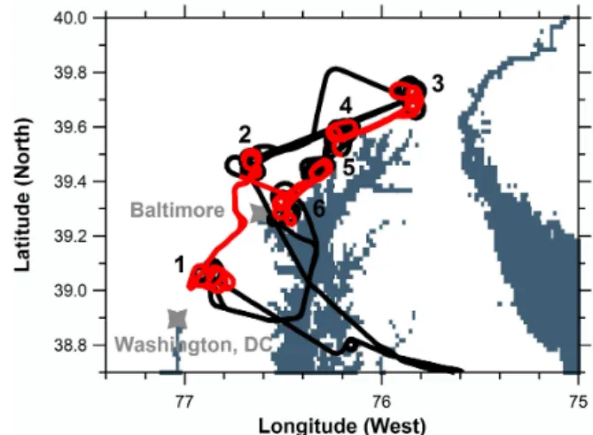
Figure 1.Flight path for flight 1. Portions below 1 km are shown
in red, and those above in black. Flights originated at NASA Wal-lops Flight Facility (southeast of the area shown) to ground sites 1 through 6 in order, with a spiral performed at each site. The cir-cuit was typically flown three times per flight before returning to Wallops. Water is denoted as blue, with the Chesapeake Bay at the center and the Delaware Bay on the right edge.
MD–Washington, D.C. region and their effect on variability in aerosol extinction.
DISCOVER-AQ (Deriving Information on Surface con-ditions from Column and Vertically Resolved Observations Relevant to Air Quality) was a multi-city NASA project designed to better elucidate the connection between satel-lite measurements and air quality by studying the variabil-ity in gas-phase and particulate pollutants in urban environ-ments. The first campaign was performed in the Baltimore– Washington region in July 2011 and combined remote-sensing instruments on the NASA Langley UC-12 flying at 9 km, ground-based observations at multiple sites through-out the region, and in situ airborne measurements from the NASA Wallops P-3B for the detailed analysis of atmospheric composition in the Baltimore–Washington urban airshed. The P-3B flight plans (Fig. 1) were consistent among the 14 flights over 29 days to provide meaningful statistics (Ta-ble 1).
DISCOVER-AQ provides a valuable data set to determine the variability in aerosol extinction throughout the region. However, it is important to note that changes in aerosol ex-tinction are not necessarily solely due to an increase or de-crease in aerosol loadings but can also be indicative of vari-ability in relative humidity and aerosol composition. Thus these data will be used to examine
1. the influence that aerosol loading, composition, and rel-ative humidity have on variability in aerosol extinction in the Baltimore–Washington region;
Table 1.DISCOVER-AQ flight dates including complete circuits
over all six sites flown.
Flight Date (2011) Circuits flown
1 1 July 3
2 2 July 3
3 5 July 3
4 10 July 3
5 11 July 2
6 14 July 3
7 16 July 2
8 20 July 3
9 21 July 3
10 22 July 3
11 26 July 3
12 27 July 3
13 28 July 3
14 29 July 3
These questions are relevant to scientists and policy makers seeking to assess the ability of satellite AOD retrievals to di-agnose ground-level air quality.
2 Experimental design
The NASA P-3B was equipped with a variety of in situ aerosol and gas-phase measurements. The current analysis uses a subset of these measurements including aerosol scat-tering, absorption, size distribution, and composition. Air was sampled with an isokinetic inlet which efficiently col-lects and transmits particles with a diameter smaller than 4 µm (McNaughton et al., 2007). Scattering coefficients at 450, 550, and 700 nm were measured with an integrating nephelometer (TSI, Inc. model 3563) and corrected for trun-cation errors according to Anderson and Ogren (1998), while absorption coefficients at 470, 532, and 660 nm were mea-sured with a particle soot absorption photometer (PSAP, Ra-diance Research) and corrected for filter scattering according to Virkkula (2010). In order to calculate extinction, the mea-sured Ångström exponent was used to adjust the scattering at 550 to 532 nm (Ziemba et al., 2013).
During sampling, the RH of the air is modified due to the temperature gradient between the outside and inside of the plane. This causes a change in the scattering coefficient due to the generally hygroscopic nature of aerosol. To provide a stable scattering signal, the sample is initially dried to ap-proximately 20 % RH utilizing a nafion drier and then sam-pled with tandem nephelometers (with and without humidi-fication) to find the dry (σscat,dryat a RHdryof approximately
20 %) and humidified scattering coefficients (σscat,wet at a
RHwet of approximately 80 %). These scattering
measure-ments are related via a single-parameter monotonic growth curve (Gasso et al., 2000):
σscat,wet=σscat,dry·
100−RH
wet
100−RHdry
−γ
, (1)
whereγ is an experimentally determined variable of the hy-groscopicity, with water uptake increasing with increasingγ. σscat,drywas corrected to 20 % RH based on Eq. (1) to account
for any variability in RHdry. Onceγ is determined, the scat-tering at ambient RH (σscat,amb, RHamb)is found from
σscat,amb=σscat,dry·
100−RH
amb
80
−γ
. (2)
Ambient RH was calculated based on measurements of wa-ter vapor concentration by an open-path diode laser hygrom-eter (Diskin et al., 2002), static temperature, and pressure. Aerosol extinction at ambient RH (σext,amb) can then be found by summingσscat,amband absorption (σabs):
σext,amb=σscat,dry·
100−RH
amb
80
−γ
+σabs. (3) The dependence of aerosol absorption on RH is highly un-certain (Redemann et al., 2001; Mikhailov et al., 2006; Brem et al., 2012) and is therefore not incorporated but likely man-ifests as only a small uncertainty in total extinction due to the fact that absorption was only a minor component of extinc-tion (4 % on average).
Ziemba et al. (2013) showed a good correlation (R2 of
0.88 based on comparison of 668 data points) between extinction measurements from the P-3B and coincident measurements performed by a high-spectral-resolution lidar (HSRL) on the UC-12. Recent work (Brock et al., 2015a; Wagner et al., 2015) has suggested an additional model for aerosol hygroscopicity known as the kappa (κext) parameter-ization. However, these two models (based onγandκext)are fairly consistent (scattering within 5 %) at RHs below 85 %, a range which comprised 96 % of the data measured by the P-3B. In addition, the good agreement between HSRL and in situ data (utilizing theγ correction scheme) suggests this is a valid model for the aerosol measured in Baltimore during DISCOVER-AQ (Ziemba et al., 2013).
Single-scattering albedo (SSA) describes the relationship between aerosol scattering and extinction:
SSA= σ scat,dry σext,dry = σ scat,dry
σscat,dry+σabs
. (4)
SSA can vary with RH (as scattering increases) but is here defined as the SSA under dry conditions (20 % RH). Thus Eq. (3) can be rewritten as
σext,amb=σext,dry
·
"
1+SSA·
100−RH
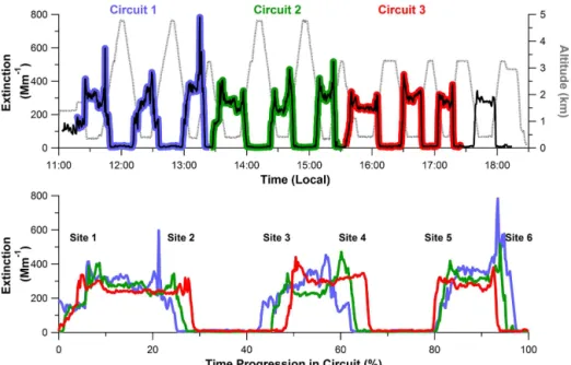
Figure 2. Time series of extinction (at ambient RH and 532 nm) and altitude (gray dashed line) for flight 9 (upper panel). Extinction
measurements during each circuit are highlighted by differing background color. Each circuit is then plotted in the bottom panel to show the changes in aerosol between the circuits. Profile locations correspond to those shown in Fig. 1.
while a pair of Particle-Into-Liquid Samplers (PILS, Brechtel Manufacturing, Inc.; Weber et al., 2001) were used to mea-sure water-soluble organic and inorganic species. The PILS captures particles in the sampled air flow into a liquid flow of deionized water. Denuders prior to the PILS removed gas-phase organic compounds (parallel-plate carbon filter denud-ers, Sunset Laboratory, Inc.) and inorganic acids and bases (annular denuders coated with sodium carbonate and phos-phoric acid, URG Corporation). Laboratory testing prior to the campaign showed the use of denuders resulted in a size cut of approximately 2 microns for the PILS systems.
The first PILS was coupled to a total organic carbon (TOC) analyzer (Sievers Model 800) to give the mass of water-soluble organic carbon (WSOC) at a 10 s time resolution. The TOC analyzer reports the organic carbon mass in µgC m−3
and not the total organic mass (which includes mass due to bonded hydrogen and oxygen atoms). Thus, to determine to-tal water-soluble organic matter (WSOM), a multiplier rang-ing from 1.6 for urban to 2.1 for non-urban aerosols must be applied (Turpin and Lim, 2001). For the present work, a value of 1.8 is used based on Hand and Malm (2007). How-ever, it should be noted that this does not include mass from any water-insoluble organic compounds.
The liquid flow from the second PILS was collected in vials at a resolution of 3.25 or 5 min for offline ion chro-matographic (IC) analysis of chloride, nitrate, nitrite, sul-fate, sodium, ammonium, potassium, magnesium, and cal-cium mass concentrations. The IC (Dionex ICS-3000 with an auto-sampler) utilized a CS12A column for cation anal-ysis and an AS11 column for anion analanal-ysis with run times of 15 and 20 min, respectively. Standards were run
periodi-cally for calibration and to ensure system stability. Dilution was measured in the PILS through the addition of lithium bromide to its water supply. Complete inorganic composition data are not available from the first three flights due to con-tamination from the sample vials; alternate vials were used for the remainder of the campaign. Aerosol size distributions were measured with an Ultra-High Sensitivity Aerosol Spec-trometer (UHSAS, Droplet Measurement Technologies) cal-ibrated with ammonium sulfate. All data are publicly avail-able from the NASA Langley Atmospheric Science Data Center (ASDC, 2015).
As the PILS is unable to measure insoluble aerosol, the measured aerosol mass is a lower limit for the actual mass. The PILS mass can be compared to the volume measured by the UHSAS utilizing a density determined based on the mea-sured mass of organics (1.2 g cm−3; Turpin and Lim, 2001)
and ammonium sulfate (1.77 g cm−3). Based on this
analy-sis, the PILS measured approximately 82 % of the aerosol mass, with the other 18 % assumed to be insoluble organic compounds. Higher insoluble organic masses are estimated for higher loadings days, with insoluble loadings near zero for low-loading days. However, this analysis has a large un-certainty due to a difference in size range measured by the two instruments and volatilization of aerosol at the PILS tip. Measurements by Sorooshian et al. (2006) show that slightly more than 10 % of the ammonium is lost in the PILS with a tip temperature of approximately 100◦C. Good
Figure 3.Vertical profiles of aerosol extinction (at ambient RH and 532 nm) for flight 9 segregated by circuit and profile site. Horizontal lines
represent the boundary layer (solid line) and buffer layer (dashed line) heights during each circuit at site 2 based on airborne measurements of the potential temperature profile.
of possible insoluble mass, this estimation is not included in future analysis due to the high uncertainty.
3 Results – mission overview
Each DISCOVER-AQ Maryland flight can be broken into two to three repetitive circuits which encompassed spirals from 0.3 to 4.5 km centered over six primary ground sites (la-belled as sites 1–6 in Fig. 1). When time permitted, additional spirals were performed at select sites at the end of the flight, resulting in two to four spirals over each site per flight. A time series of aerosol extinction during flight 9 highlights an altitude dependence of aerosol scattering, with values oscil-lating between near zero in the free troposphere and greater than 200 Mm−1in the mixing layer (Fig. 2).
The repetitive flight plan allows for the analysis of dif-ferences in aerosol properties and their vertical distributions at each site as source profiles and boundary layer dynamics changed during the day, as seen for flight 9 in Fig. 3. During the first circuit (11:00–13:30 local time), a mixed layer up to 1.5 km is seen, capped by a residual layer between 1.5 and 2.5 km. Surface heating causes the two layers to merge by the time the second circuit was performed (13:30–15:30), with fairly constant extinction to 1.5 km and a gradual decrease to near-zero extinction by 2.5 km. Circuit 3 (15:30–17:30) had constant extinction below 1.5 km but little indication of a residual layer. In addition, the profiles among the sites be-come more homogeneous as the day progresses (Fig. 3). In general, the mixing layer was consistently greater than 1 km throughout the flights; therefore, data below 1 km are used as a measure of mixing layer aerosol properties.
Aerosol mass loadings varied by a factor of 6 (Fig. 4) be-tween the flights, with average aerosol mass in the lowest 1 km ranging from 3.8 to 26 µg m−3. Aerosol optical
mea-surements varied by an even greater amount, with ambi-ent aerosol extinction in the lowest 1 km ranging from 20 to 290 Mm−1 and AODs (calculated from the integration
of the extinction profile) ranging from 0.05 to 0.57. In situ AOD measurements showed good agreement (within 0.04)
Figure 4.Average AOD (at ambient RH) along with boundary layer
(below 1 km) extinction, aerosol mass, effective radius, and compo-sition for each of the 14 flights. Aerosol mass and compocompo-sition data are not available for the first three flights. Flights with predomi-nantly westerly transport from the Ohio River Valley are indicated by stars at the top of the plots.
Figure 5.Average vertical profiles of aerosol extinction (at ambient
RH and 532 nm) for all flights, with flights 9 and 14 highlighted (left panel). These profiles can then be normalized to the total aerosol loading (AOD) to get the normalized vertical profile (right panel, arbitrary units).
layer aerosol loading. Flight 14 had a deeper aerosol layer and more aerosol in an elevated layer than flight 9 (Fig. 5); thus flight 14 had a higher AOD despite having less near-surface extinction than flight 9. Other near-surface-independent factors influencing AOD may include aerosol cloud process-ing. Indeed, Eck et al. (2014) observed large increases in AOD (average of 25 %) in the vicinity of non-precipitating cumulus clouds. Consistent with these findings, in situ mea-surements showed increases in aerosol scattering, volume, and mass in spirals measured before and after cloud forma-tion. These included a doubling of water-soluble organics and 50 % increase in sulfate.
In general, the fraction of aerosol measured was primarily a mixture of WSOM (campaign average of 57 % by mass, Fig. 4), sulfate (23 %), and ammonium (10 %), with mi-nor contributions from nitrate (2.1%), BC (2.2 %), chloride (2.0 %), and sodium (1.3 %). The molar ratio of ammonium to sulfate was 1.92, showing that sulfate is almost completely neutralized as ammonium sulfate, (NH4)2SO4, with minimal
bisulfate, (NH4)HSO4. Further, this ratio is higher (above 2)
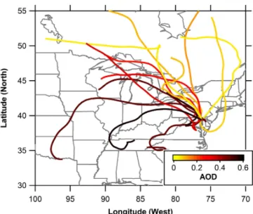
if PILS volatilization of ammonium (12 % loss of mass; Sorooshian et al., 2006) and sulfate (1 % loss) is considered. Composition varied between flights with polluted days (as noted in Fig. 4) exhibiting a higher fraction of ammonium and sulfate. Back-trajectory analysis with the Hybrid Single-Particle Lagrangian Integrated Trajectory Model (HYSPLIT; Draxler and Hess, 1998; Draxler and Rolph, 2015) suggested these high-aerosol-loading days were related to long-range transport from the Ohio River Valley (Fig. 6), which has en-hanced sulfur dioxide emissions due to a high density of coal-fired power plants in the region (Hand et al., 2012). These days were generally associated with low-pressure systems to the northwest of the study region. Conversely, low-loading days tended to have northerly flow due to high-pressure sys-tems to the west.
The flights with transport from the west and higher aerosol loadings (starred in Fig. 4) were found to have relatively
Figure 6.72 h back trajectories based on HYSPLIT for the first
circuit of each flight at site 5 at an altitude of 1 km colored by the average AOD measured during that flight.
more sulfate (28 % of mass compared to 15 % for clean days) and ammonium (polluted, 11 %; clean, 7.5 %) and less or-ganics (polluted, 52 %; clean, 65 %). Less polluted days had higher percentages of nitrate (polluted, 1.1 %; clean, 3.9 %) and BC (polluted, 2.0 %; clean, 2.7 %). The higher BC mass percentage also leads to higher absorption relative to scat-tering and therefore lower SSA on these less polluted days (polluted, 0.98; clean, 0.93; Fig. 7). However, on an absolute basis the polluted days had higher BC and absorption than on the clean days. Average BC concentrations for the en-tire month were 240 ng m−3in the lowest 1 km, decreasing
to 35 ng m−3in the free troposphere (above 3 km).
The polluted flight days also had higherγ values (Fig. 7, Eq. 5). This water uptake is largely dependent on aerosol composition, with soluble organics having lower hygroscop-icity than inorganic compounds. This can be seen as an in-verse relationship with γ=0.60−0.0042×organic mass
fraction (Fig. 8). These values are intermediate between mea-surements made in other urban areas (Asia and USA – Quinn et al., 2005; Texas – Massoli et al., 2009) and in the remote atmosphere (the Indian Ocean – Quinn et al., 2005). Differ-ences are likely due to differDiffer-ences in the measurement of or-ganics; the current study uses PILS to measure only water-soluble organics, while the other studies use aerosol mass spectrometry or thermo-optical methods which are sensitive to all organic species. In addition to an elevated γ, high-loading days were typically more humid (64±7 % compared
low-Figure 7. Average profiles for extinction (at ambient RH and 532 nm),γ, SSA, and composition for all flights (black line), days with predominantly westerly transport from the Ohio River Valley (red line), and days with northerly transport (blue line).
Figure 8. Relationship betweenγ (at 532 nm) and organic mass fraction for the present study (data below 1 km), Texas (Massoli et al., 2009), the western Pacific, the northeast USA, and the Indian Ocean (Quinn et al., 2005). The organic mass fraction is found by dividing the WSOM by the total mass measured by the PILS and SP2. Other studies used organic mass measured by aerosol mass spectrometer or thermo-optical methods. The ratio of scattering at 80 % RH to 20 % [f(RH)] is shown on the righty axis (note the irregular spacing).
loading days. The highest daily-averaged water content of aerosol extinction was 40 % measured during flight 8.
Aerosol mass is the primary measurement of aerosol load-ing and the basis on which ground air quality is regulated. Boundary layer dry extinction, ambient extinction, and AOD are additional measures of aerosol loading but incorporate an increasing amount of confounding factors. For instance, dry extinction is dependent on the aerosol mass loading in addi-tion to aerosol size and composiaddi-tion. Ambient extincaddi-tion is dependent on these same factors plus the aerosol hygroscop-icity and RH. Finally, AOD is also dependent on the vertical distribution of aerosols and RH. Aerosol mass loading, dry extinction (not shown), ambient extinction, and AOD follow similar trends (Fig. 4), suggesting that aerosol mass loadings are the primary factor controlling day-to-day variability in
aerosol optical properties. However, aerosol mass measure-ments via PILS do not account for insoluble aerosol. Dry mass extinction efficiencies calculated from extinction and mass measurements were variable, ranging between 3.2 and 8.3 m2g−1. The highest mass extinction efficiencies
(mea-sured on high-loading days) likely are indicative of the pres-ence of insoluble organic material. Therefore, because of the variable quantity of insoluble mass and the low time resolu-tion of the PILS measurements, future analysis will use the dry extinction as a proxy for aerosol loadings.
4 Results – regional variability
Aerosol extinction varied not only on a temporal basis (Fig. 4) but also spatially. Because there is such a large differ-ence in aerosol loadings, optical properties (related to com-position), and RH between flights, using campaign averages would distort the spatial trends. Therefore, each circuit con-sisting of spirals over six ground sites is treated as a separate “snapshot” of the region, and the properties measured over each site are normalized to the circuit average to study the spatial variability. Data below 1 km pressure altitude were used from 34 circuits for which spirals were performed over all six sites (absorption measurements were not available for one additional circuit, and therefore it was not included in this analysis).
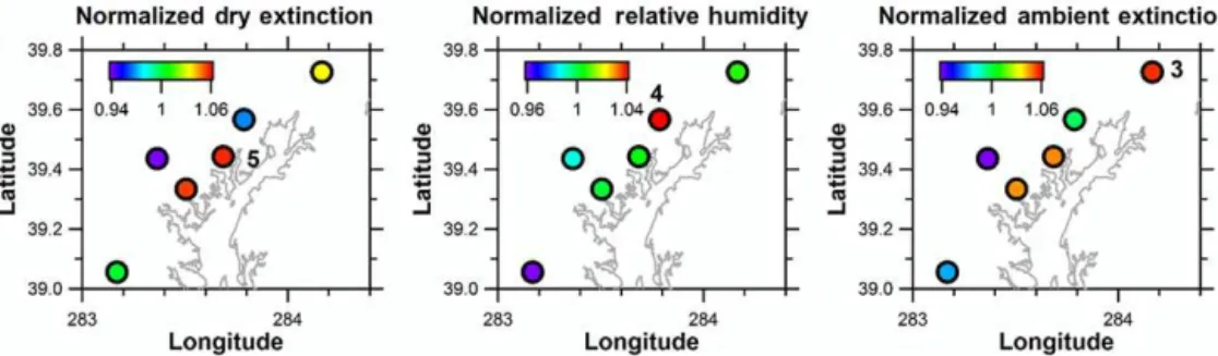
Figure 9.Average normalized 532 nm dry extinction (left panel), RH (center), and 532 nm ambient extinction (right) for all of the circuits
(data are normalized to the average value for that circuit). The site with the maximum value is labelled.
in such a way that extinction is constant throughout the re-gion.
However, in order to study aerosol variability, it is impor-tant to analyze each circuit individually (and not as a cam-paign average as done in Fig. 9). Equation (5) shows the dependence of aerosol ambient extinction on aerosol load-ing (σext,dry), composition (SSA andγ ), and RH, and it can
be used as a simple model to determine the factors control-ling aerosol ambient extinction. From this, an assessment of the accuracy needed for each of these parameters to relate aerosol extinction (which can be derived from satellite mea-surements) to aerosol loading can be performed. In order to determine the relative importance of aerosol loading, compo-sition, and RH on extinction, the partial derivatives of Eq. (5) can be determined:
∂σext,amb
∂σext,dry
=1+SSA·
100−RH
amb 80 −γ −1 ! , (6) ∂σext,amb
∂SSA =σext,dry·
100−RH
amb 80 −γ −1 ! , (7) ∂σext,amb ∂RH =
σext,dry·SSA·γ 80
100−RH
amb
80
−γ−1
, (8) ∂σext,amb
∂γ = −σext,dry·SSA·
100−RH
amb
80
−γ
·ln
100−RH
amb
80
. (9)
As expected, ambient extinction is linear with dry extinction (the partial derivative does not contain σext,dry). The
posi-tive linear dependence on SSA shows that, if all other vari-ables are held constant, as SSA increases scattering becomes a larger fraction of extinction and at any RH above 20 % will cause an increase in extinction due to water uptake. The de-pendence on RH andγ are both nonlinear, and thus their ef-fects are most important when the RH is high or the aerosol is very hygroscopic.
Figure 10.Average 532 nm ambient extinction, dry extinction, and
RH below 1 km during spirals over the six sites during flights 1 and 14.
Equations (6) through (9) can be combined to give the total differential forσext,amb:
dσext,amb=∂σext,amb
∂σext,dry
·dσext,dry+∂σext,amb
∂SSA ·dSSA
+∂σext,amb
∂RH ·dRH+
∂σext,amb
∂γ ·dγ . (10) Assuming that the four variables are independent,
s σext,amb=
∂σ ext,amb ∂σext,dry
·s σext,dry
2
+
∂σ
ext,amb
∂SSA ·s (SSA) 2
+
∂σ
ext,amb
∂RH ·s (RH) 2
+
∂σ
ext,amb
∂γ ·s (γ ) 2
1/2
, (11)
Figure 11.Relative contribution of dry extinction and RH to the spatial variability in ambient extinction as a function of RH (left) and to the
diurnal variability (right). Diamonds represent the average relative contributions for 10 % RH increments.
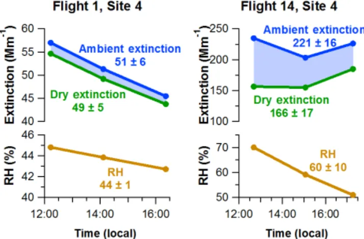
Figure 12.Trends in 532 nm ambient extinction, dry extinction, and
RH below 1 km during spirals at site 4 during flights 1 and 14.
contribution (RC) of dry aerosol scattering to the variability in ambient extinction in the region can then be found by
RC σext,dry=
∂σ
ext,amb
∂σext,dry ·s σext,dry
2
s σext,amb2
. (12)
Using this method, the RC for each of the four variables can be determined for each circuit.
In order to determine the relative contribution of each fac-tor to the variability in ambient aerosol extinction, each cir-cuit was analyzed separately. Shown in Fig. 10 are two ex-treme cases. During flight 1, ambient relative humidity was low (37±4 %), resulting in little water uptake (the shaded
portion on the upper panel). Thus variability in dry extinc-tion (aerosol loading) is the major contributor (RC(σext,dry)=
99 %) to variability in ambient extinction. The second case during flight 14 shows a period of high RH (64±8 %).
Wa-ter uptake was substantial and greatest at site 3, where the RH is the highest. In this case, the variability in aerosol ex-tinction is dependent not only on variability in dry exex-tinction (41 %) but also on relative humidity (57 %).
On average, aerosol loading (dry extinction) accounted for 88 % of the spatial variability in extinction, with 27 of the 34
complete circuits having RC(σext,dry)above 80 % (Fig. 11). Variability in RH only accounted for 10 % of the ambient extinction variability on average, with only five circuits hav-ing RC(RH) greater than 20 %. Four of these cases where RH had a large effect on ambient extinction variability cor-responded to days with high RH (above 60 %). This is due to the nonlinearity of extinction with respect to RH (Eq. 8). Thus at low relative humidities, changes in RH minimally impact ambient extinction. Conversely, when RHs are high, small changes can produce large variations in ambient ex-tinction. Changes inγ and SSA were smaller contributors to ambient extinction variability (1.3 % and less than 0.1 % on average, respectively).
5 Results – diurnal variability
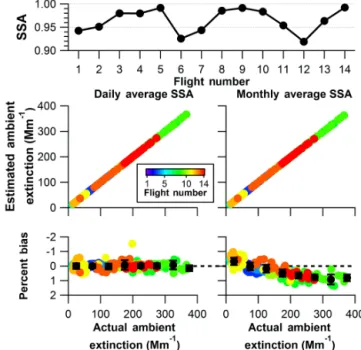
Figure 13. Averageγ for each flight (top) along with estimated ambient extinction and percent bias if the flight-average (left) and campaign-average (right)γare used.
and less than 0.1 %, respectively). However, RC(RH) values greater than 90 % were measured during flight 9 (highest or-ange markers on the right panel of Fig. 11), a day with high RH and highly variable RH.
6 Discussion
The conversion of extinction at ambient RH to extinction at a reduced (“dry”) RH is important in relating remote-sensing measurements of ambient extinction to dry aerosol mass. Though the analysis above shows that variability in γ and SSA are only minor contributors to ambient tion variability, converting between ambient and dry extinc-tion requires knowledge of both parameters, as evidenced by Eq. (3). However, both γ and SSA are not routinely mea-sured at air quality monitoring sites. So the question could be asked, “at what frequency (both spatially and temporally) do γ and SSA need to be known to determine the proper RH conversion?” This can be examined by analyzing the DISCOVER-AQ Maryland data recorded below 1 km and determining how using more averaged data yields differing ambient aerosol extinctions.
As a result of changes in composition seen in Fig. 4, γ varied between 0.14 (flight 1) and 0.47 (flight 8), with an av-erage of 0.32 (Fig. 13). Comparing the ambient extinction calculated during each spiral with the extinction calculated using the daily-averageγ resulted in a bias of±1.6 % in
am-bient extinction, with no clear trend with respect to aerosol extinction. Using the monthly average for the entire region
Figure 14.Average SSA for each flight (top) along with estimated
ambient extinction and percent bias if the flight-average (left) and campaign-average (right) SSA are used.
Table 2.Percent bias in ambient extinction based on daily and
monthly averaging of contribution variables.
Variable Percent bias
based on averaging
Daily Monthly
Dry extinction 22 111
RH 6.2 10.7
γ 1.6 6.8
SSA 0.21 0.49
causes a bias of ±6.8 % (Table 2) with deviations of up
to 27 % at high aerosol extinction becauseγ tended to be higher on high-aerosol-loading days (Fig. 8). We conclude that spatialγdifferences in the Baltimore region are not large enough to cause significant biases in deriving dry extinction from ambient values. However, day-to-day variability inγ can cause large discrepancies. Thus it appears that a single daily measurement ofγ(or one based on compositional mea-surements, Fig. 8) is able to be used for AOD-to-PM2.5
cor-relations over the study region (on the order of 1400 km2)
within an uncertainty of 2 %.
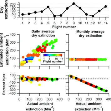
extinc-Figure 15.Average dry extinction for each flight (top) along with
estimated ambient extinction and percent bias if the flight-average (left) and campaign-average (right) dry extinction are used.
tion calculated during each spiral with the extinction cal-culated using the daily-average SSA resulted in a bias of
±0.2 % in ambient extinction, showing that regional
vari-ability in SSA was not high enough to make a significant difference. Using the monthly average for the entire region produces biases of±0.5 % with deviations of up to 1.0 % at
high aerosol extinction.
Doing the same analysis for dry aerosol extinction or RH shows markedly different results (Figs. 15 and 16, Table 2). The use of a daily-average dry extinction causes a bias of
±22 %, showing that regional variation in aerosol loading
must be accounted for. Utilizing a monthly average extinc-tion causes discrepancies of ±111 % due to the large
day-to-day variability in aerosol loading. Biases based on lim-ited knowledge of RH were smaller, with±6.2 % for daily
and 11 % for monthly RH. Thus, Table 2 gives a hierarchy of factors for variability in extinction measurements: loading >RH> γ >SSA.
An analysis of the effects of aerosol and meteorological parameters on AOD in the southeastern USA based on 37 airborne profiles (Brock et al., 2015b) shows similar trends in the significance of factors, with aerosol mass being the most important. Relative humidity had a nonlinear signifi-cance on AOD, with the greatest signifisignifi-cance for extremely humid conditions (the 90th percentile RH profiles). Varying aerosol size parameters and the vertical distribution of the aerosols resulted in moderate AOD changes, while AODs were largely insensitive to refractive index in a fashion
sim-Figure 16.Average RH for each flight (top) along with estimated
ambient extinction and percent bias if the flight-average (left) and campaign-average (right) RH are used.
ilar to the present findings of SSA as a minor contributor to extinction variability.
7 Conclusions
Measurements made in the Baltimore–Washington, D.C. re-gion during DISCOVER-AQ in July 2011 can be general-ized as follows: on days influenced by transport from the Ohio River Valley, aerosol loadings were higher (aerosol mass concentrations of 18.7±4.4 µg m−3 and AODs of
0.43±0.12) and the aerosol were more hygroscopic (γ of
0.36±0.07) because of a larger percentage of ammonium
and sulfate (38 % of water-soluble mass) in comparison to days impacted by northerly transport (aerosol masses of 5.4±1.3 µg m−3, AODs of 0.08±0.03, γ of 0.26±0.09,
20 % ammonium and sulfate). In both cases, the regional and diurnal variability in aerosol extinction are controlled pri-marily by changes in aerosol loadings. However, on days as-sociated with westerly transport (which also were more hu-mid) variability in RH also contributed significantly to the regional (14 %) and diurnal (22 %) variability in extinction. Thus changes in AOD cannot directly be seen as changes in PM2.5but must take into account spatial and temporal vari-ability in RH.
able aerosol composition and vertical distributions (Engel-Cox et al., 2004).
Acknowledgements. This research was funded by NASA’s Earth Venture-1 Program through the Earth System Science Pathfinder (ESSP) Program Office. We thank the DISCOVER-AQ Science Team, especially the pilots and flight crews of NASA’s P-3B. Boundary layer heights based on airborne measurements of the potential temperature profile were provided by Don Lenschow of the University Corporation for Atmospheric Research (UCAR). Thanks also to Joshua DiGangi and Michael Shook (both of NASA Langley) for valuable discussions during manuscript preparation.
Edited by: P. DeCarlo
References
Al-Saadi, J., Szykman, J., Pierce, R. B., Kittaka, C., Neil, D., Chu, D. A., Remer, L., Gumley, L., Prins, E., Weinstock, L., MacDon-ald, C., Wayland, R., Dimmick, F., and Fishman, J.: Improving National Air Quality Forecasts with Satellite Aerosol Observa-tions, B. Am. Meteorol. Soc., 86, 1249–1261, 2005.
Anderson, T. L. and Ogren, J. A.: Determining Aerosol Radiative Properties using the TSI 3563 Integrating Nephelometer, Aerosol Sci. Tech., 29, 57–69, 1998.
ASDC: NASA Airborne Science Data for Atmospheric Compo-sition: DISCOVER-AQ, available at: http://www-air.larc.nasa. gov/cgi-bin/ArcView/discover-aq.dc-2011 (last access: 14 Jan-uary 2016), 2015.
Brem, B. T., Mena Gonzalez, F. C., Meyers, S. R., Bond, T. C., and Rood, M. J.: Laboratory-Measured Optical Properties of In-organic and Organic Aerosols at Relative Humidities up to 95 %, Aerosol Sci. Tech., 46, 178–190, 2012.
Brock, C. A., Wagner, N. L., Anderson, B. E., Attwood, A. R., Beyersdorf, A., Campuzano-Jost, P., Carlton, A. G., Day, D. A., Diskin, G. S., Gordon, T. D., Jimenez, J. L., Lack, D. A., Liao, J., Markovic, M. Z., Middlebrook, A. M., Ng, N. L., Perring, A. E., Richardson, M. S., Schwarz, J. P., Washenfelder, R. A., Welti, A., Xu, L., Ziemba, L. D., and Murphy, D. M.: Aerosol optical properties in the southeastern United States in summer – Part 1: Hygroscopic growth, Atmos. Chem. Phys. Discuss., 15, 25695– 25738, doi:10.5194/acpd-15-25695-2015, 2015a.
Brock, C. A., Wagner, N. L., Anderson, B. E., Beyersdorf, A., Campuzano-Jost, P., Day, D. A., Diskin, G. S., Gordon, T. D., Jimenez, J. L., Lack, D. A., Liao, J., Markovic, M., Middle-brook, A. M., Perring, A. E., Richardson, M. S., Schwarz, J. P., Welti, A., Ziemba, L. D., and Murphy, D. M.: Aerosol optical
Crumeyrolle, S., Chen, G., Ziemba, L., Beyersdorf, A., Thornhill, L., Winstead, E., Moore, R. H., Shook, M. A., Hudgins, C., and Anderson, B. E.: Factors that influence surface PM2.5values in-ferred from satellite observations: perspective gained for the US Baltimore–Washington metropolitan area during DISCOVER-AQ, Atmos. Chem. Phys., 14, 2139–2153, doi:10.5194/acp-14-2139-2014, 2014.
Diskin, G. S., Podolske, J. R., Sachse, G. W., and Slate, T. A.: Open-path airborne tunable diode laser hygrometer, Proceedings of SPIE, 196, 4817, doi:10.1117/12.453736 2002.
Draxler, R. R. and Hess, G. D.: An overview of the HYSPLIT-4 modeling system of trajectories, dispersion, and deposition, Aust. Meteorol. Mag., 47, 295–308, 1998.
Draxler, R. R. and Rolph, G. D.: NOAA Air Resources Labora-tory HYSPLIT (HYbrid Single-Particle Lagrangian Integrated Trajectory), available at: http://ready.arl.noaa.gov/HYSPLIT.php (last access: 14 January 2016), 2015.
Eck, T. F., Holben, B. N., Reid, J. S., Arola, A., Ferrare, R. A., Hostetler, C. A., Crumeyrolle, S. N., Berkoff, T. A., Welton, E. J., Lolli, S., Lyapustin, A., Wang, Y., Schafer, J. S., Giles, D. M., Anderson, B. E., Thornhill, K. L., Minnis, P., Pickering, K. E., Loughner, C. P., Smirnov, A., and Sinyuk, A.: Observations of rapid aerosol optical depth enhancements in the vicinity of pol-luted cumulus clouds, Atmos. Chem. Phys., 14, 11633–11656, doi:10.5194/acp-14-11633-2014, 2014.
Engel-Cox, J. A., Holloman, C. H., Coutant, B. W., and Hoff, R. M.: Qualitative and quantitative evaluation of MODIS satellite sensor data for regional and urban scale air quality, Atmos. Environ., 38, 2495–2509, 2004.
EPA: National Ambient Air Quality Standards, available at: http://www3.epa.gov/ttn/naaqs/criteria.html, last access: 14 Jan-uary 2016.
Gasso, S., Hegg, D. A., Covert, D. S., Collins, D., Noone, K. J., Os-trom, E., Schmid, B., Russell, P. B., Livingston, J. M., Durkee, P. A., and Jonsson, H.: Influence of humidity on the aerosol scat-tering coefficient and its effect on the upwelling radiance during ACE-2, Tellus B, 52, 546–567, 2000.
Hand, J. L. and Malm, W. C.: Review of aerosol mass scattering ef-ficiencies from ground-based measurements since 1990, J. Geo-phys. Res., 112, D16203, doi:10.1029/2007JD008484, 2007. Hand, J. L., Schichtel, B. A., Malm, W. C., and Pitchford, M.
L.: Particulate sulfate ion concentration and SO2 emission trends in the United States from the early 1990s through 2010, Atmos. Chem. Phys., 12, 10353–10365, doi:10.5194/acp-12-10353-2012, 2012.
Holben, B. N., Eck, T. F., Slutsker, I., Tanre, D., Buis, J. P., Set-zer, A., Vermote, E., Reagan, J. A., Kaufman, Y., Nakajima, T., Lavenu, F., Jankowiak, I., and Smirnov, A.: AERONET-A feder-ated instrument network and data archive for aerosol characteri-zation, Remote Sens. Environ., 66, 1–16, 1998.
Liu, Y., Sarnat, J. A., Kilaru, V., Jacob, D. J., and Koutrakis, P.: Es-timating Ground-Level PM2.5in the Eastern United States Us-ing Satellite Remote SensUs-ing, Environ. Sci. Technol., 39, 3269– 3278, 2005.
Massoli, P., Bates, T. S., Quinn, P. K., Lack, D. A., Bay-nard, T., Lerner, B. M., Tucker, S. C., Brioude, J., Stohl, A., and Williams, E. J.: Aerosol optical and hygroscopic prop-erties during TexAQS-GoMACCS 2006 and their impact on aerosol direct radiative forcing, J. Geophys. Res., 114, D00F07, doi:10.1029/2008JD011604, 2009.
McNaughton, C. S., Clarke, A. D., Howell, S. G., Pinkerton, M., Anderson, B., Thornhill, L., Hudgins, C., Winstead, E., Dibb, J. E., Scheuer, E., and Maring, H.: Results from the DC-8 Inlet Characterization Experiment (DICE): Airborne Versus Surface Sampling of Mineral Dust and Sea Salt Aerosols, Aerosol Sci. Tech., 41, 136–159, 2007.
Mikhailov, E. F., Vlasenko, S. S., Podgorny, I. A., Ramanathan, V., and Corrigan, C. E.: Optical properties of soot–water drop agglomerates: An experimental study, J. Geophys. Res., 111, D07209, doi:10.1029/2005JD006389, 2006.
Quinn, P. K., Bates, T. S., Baynard, T., Clarke, A. D., Onasch, T. B., Wang, W., Rood, M. J., Andrews, E., Allan, J., Carrico, C. M., Coffman, D., and Worsnop, D.: Impact of particulate organic matter on the relative humidity dependence of light scattering: A simplified parameterization, Geophys. Res. Lett., 32, L22809, doi:10.1029/2005GL024322, 2005.
Redemann, J., Russell, P. B., and Hamill, P.: Dependence of Aerosol Light Absorption and Single-Scattering Albedo on Ambient Rel-ative Humidity for Sulfate Aerosols with Black Carbon Cores, J. Geophys. Res., 106, 27485–27495, 2001.
Sorooshian, A., Brechtel, F. J., Ma, Y. L., Weber, R. J., Corless, A., Flagan, R. C., and Seinfeld, J. H.: Modeling and characterization of a particle-into-liquid sampler (PILS), Aerosol Sci. Tech., 40, 396–409, 2006.
Turpin, B. J. and Lim, H.-J.: Species Contributions to PM2.5Mass Concentrations: Revisiting Common Assumptions for Estimat-ing Organic Mass, Aerosol Sci. Tech., 35, 602–610, 2001. Vahlsing, C. and Smith, K. R.: Global review of national ambient
air quality standards for PM10and SO2(24 h), Air Quality, At-mosphere & Health, 5, 393–399, 2012.
van Donkelaar, A., Martin, R. V., and Rokjin, J. P.: Estimat-ing ground-level PM2.5using aerosol optical depth determined from satellite remote sensing, J. Geophys. Res., 111, D21201, doi:10.1029/2005JD006996, 2006.
Virkkula, A.: Correction of the calibration of the 3-wavelength Par-ticle Soot Absorption Photometer (3λPSAP), Aerosol Sci. Tech., 44, 706–712, 2010.
Wagner, N. L., Brock, C. A., Angevine, W. M., Beyersdorf, A., Campuzano-Jost, P., Day, D., de Gouw, J. A., Diskin, G. S., Gor-don, T. D., Graus, M. G., Holloway, J. S., Huey, G., Jimenez, J. L., Lack, D. A., Liao, J., Liu, X., Markovic, M. Z., Middle-brook, A. M., Mikoviny, T., Peischl, J., Perring, A. E., Richard-son, M. S., RyerRichard-son, T. B., Schwarz, J. P., Warneke, C., Welti, A., Wisthaler, A., Ziemba, L. D., and Murphy, D. M.: In situ ver-tical profiles of aerosol extinction, mass, and composition over the southeast United States during SENEX and SEAC4RS: ob-servations of a modest aerosol enhancement aloft, Atmos. Chem. Phys., 15, 7085–7102, doi:10.5194/acp-15-7085-2015, 2015. Weber, R. J., Orsini, D., Daun, Y., Lee, Y.-N., Klotz, P. J., and
Brechtel, F.: A Particle-into-Liquid Collector for Rapid Mea-surement of Aerosol Bulk Chemical Composition, Aerosol Sci. Tech., 35, 718–727, 2001.