Tree Structured Symmetrical Systems of Linear
Equations and their Graphical Solution
define the topology of the graph which represents the SLE. IfAis very sparse then the graph will have very
few interconnections. It turns out that many physical systems solved using linear systems are very sparse. In particular, in electrical power systems, the matrices which represent transmission networks are very spar-se. This is the main reason why sparsity techniques have been improved by research whose goal is to solve efficiently the actual state of the power system; such as the best elimination ordering [6], [9]. Sparsity techniques have been around since at least 1970 using a technique known as bifactorization [10]. The main principles used in matrix bifactorization are strongly directed toward exploiting the underlying matrix graph.
Therefore in order to approach the solution using its graph representation, first an appropriate model has to be derived. This model has to be able to represent the complete SSLE elements (i.e. A,x,and b). The model proposed in this document is based on
a per equation basis. This representation is given in figure 1.
a
x
i..+ +..+
a
ijx
j+..=b
ix
ia
ii ib
a
jia
ijii
Figura 1. Conversion from a linear system of equations to its graph model
In this model an equation is represented by two components: a node and a set of links. The node is a well defined component which consists of two subcomponents: a circle consisting of two half parts and an arc. The upper part of the circle represents the variable related to this equation which has to be solved by the system (i.e. xi) and the lower part represents the coefficient related to this variable in equation i (i.e. aii). The arc represents the i−th component inb (i.e.bi). The second part depends on
the SLE topology and is represented by links which connect the nodes. These links will be denoted as (i, j)whereiandjrepresent the row and the column number respectively. There can be zero or more links which connect the node with some other nodes in
the graph. Each link has an associated value for the coefficient located in the row i column j (i.e. aij). Perhaps it is a little absurd to consider the case where there are no external links. However, as will be shown later, this is the basic configuration which will always be pursued in order to solve the SLE.
III. Tree Structured Symmetric Systems of Linear Equations and Its Graphical Repre-sentation.
Tree structured symmetrical systems of linear equations (TSSSLE) are SLE where the graph repre-senting the SLE is a tree. Based on this structure, efficient algorithms can be derived in order to solve this kind of systems. These algorithms emerge natu-rally, just by exploiting the properties of trees. This kind of graphs have been applied to solve electrical distribution networks whose main characteristic is its radial shape (i.e. no loops exists in the network). Therefore a tree structure can be derived for the SLE representing these systems. Algorithms to solve dif-ferent problems with difdif-ferent degree of complexity have been proposed for distribution networks based on this structure in [5], [4], [2], [7].
A tree-shaped graph has to be free of loops. This work does not deal with how to identify and remove loops from graphs. Let us instantiate equation 1 with equation 2.
0,5 0 −1 0 0 2 −1 0
−1 −1 1 −1
0 0 −1 4 x1 x2 x3 x4 = 0 0 −5 0 (2)
whose solution for the TSSSLE denoted by equa-tion 2 is given by 3
x1 x2 x3 x4 = 40/7 10/7 20/7 5/7 (3)
Applying the model defined in figure 1, leads to the graph shown in figure 2 which which complains with the TSSSLE properties.
x =?1 x =?2
−1
3
x =?4
1 −5
0 4
x =?
−1 −1
0 0.5 0 2
Figura 2. Graph corresponding to the system defined by equation 2
Gaussian elimination will be used as the main tool to solve the system.
IV. Gaussian Elimination and Its graphical Interpretation
Gaussian elimination is a general method to solve a SLE. It consists of the iterative application of elementary row operations which lead the system to an echelon form. This is achieved by modifying each of the elements which do not belong to the column and row to the equation under reduction. These elements are modified using expression 4.
a′ij =aij−aikakj akk
(4)
Gaussian elimination can be regarded as a matrix transformation from Rn×n→ R(n−1)×(n−1). The re-sulting system has all the information needed to solve the subsystem resulting from the transformation. Let us define Γk as the set of nodes adjacent to nodek. Then, the maximum number of elements generated in the elimination is given by equation 5 .
Nk= |Γk|(|Γk| −1)
2 (5)
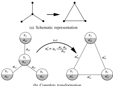
IV-A. Special Cases for Gaussian Elimination
As mentioned previously, Gaussian elimination has two main costs: updating and link creation. The first one is unavoidable but the second one can be optimised if an elimination order is achieved such
that the number of links created are minimal, or in the ideal case no links are created. There are three special cases which deserve special attention. The first one is shown in figure 3. This is the well known as star-delta transformation in electrical engineering. Here |Γk|= 3 and by equation 5 at most three new links will be generated.
(a) Schematic representation
a’ 44 a’ 11 a’ 14 a’ 12 a’ 24 a’ 1 x
x 3
x 4
2 x 22 a 33 a 44 a 11 a 13 a 34 a 23 a ij
a’ =a −ij a ika kj kk
a k=3
x
x 4
2
x
22 1
(b) Complete transformation
Figura 3. Gaussian elimination for|Γk|= 3.
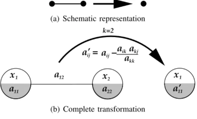
The second one is shown in figure 4. This is the well known series reduction in electrical engineering. Here |Γk| = 2 and by equation 5 at most one new link will be generated.
(a) Schematic representation
x 22 a 33 a 11 a 13
a a 23
1
x x 2
22
a’
11
a’ a’12
ij
a’ =a −ij a ika kj kk
a k=3
1
x
x 3
2
(b) Complete transformation
Figura 4. Gaussian elimination for|Γk|= 2.
TSSSLE as the leafs can be regarded as dangling nodes. Once they are reduced, then the nodes where they were dangling from can be reduced, and so on.
(a) Schematic representation
x
22
a
11
a
12
a x 1
11
a’
ij
a’ =a −ij a ika kj kk
a
k=2
1
x 2
(b) Complete transformation
Figura 5. Gaussian elimination for|Γk|= 1.
V. Graph-based Solution for Tree Structured Symmetric Systems of Linear Equations
A tree is a special kind of graph whose main characteristic is the absence of loops. A standard representation for a tree is presented in figure 6. A tree has n layers, n ≥ 1, numbered from 0 to n−1. The number of layers represents its depth. A functionlayer(x)can be defined to express the layer where node x is located, for instancelayer(E) = 2. Another useful function is parent(x) which returns the node where node x is hanging from or nil if it has no parent, for instance parent(E) = B and parent(A) =nil.
3 2 1 Layer
0
C B
D
H I J K L M N O
E F G
A
Figura 6. An example of a tree.
Let us denote Υi as the set of indices j which corresponds to variables xj which are hanging from
xi as denoted by equation 6 (i.e. the childrenof xi).
Υi={j:∃(i, j), parent(i)6=j} (6)
For instance ΥA={B, C}, andΥG={N, O} in figure 6. Based on these definitions, the nodes in a tree can be classified in three types
rootnode: There is just one of them in the graph such that layer(root) = 0 andparent(root) = nil. For instance the root node in figure 6 isA (in black),
internalnode: are those nodesxsuch thatΥx 6=
∅ andx6=root. The set of internal nodes,I, in figure 6 is {B, C, D, E, F, G} (in gray),
terminal node: also called leaf node, are those
nodes x where Υx = ∅. Therefore the set L representing the leaf nodes in figure 6 is {H, I, J, K, L, M, N, N, O} (in white).
This kind of graphs are one of the most use-ful structures in computer science. Their application spans from context-free grammar analysers in com-piler theory, XML representation in internet techno-logies, and so on. A common characteristic about those applications is that only the leaf nodes have real information. However, when applied to TSSSLEs, the internal nodes will have some information which need to be processed in order to solve the SLE.
It is very important to preserve the tree structure of the system in the reduction process. The best way to reduce these graphs is by finding an order which does not generate new elements at all. From figures 3, 4 and 5 a basic fact can be asserted. The only reductions which do not generate new elements are those which are applied to nodes k where |Γk| = 1. Therefore those are the ideal candidates to apply the elimination process.
Gaussian elimination when applied to all nodes j where j ∈Υi, is expressed in equations 7 and 8 for the coefficient corresponding to variable xi and the independent term respectively.
a′
ii=aii− X
j∈Υi
a2 ij
ajj (7)
b′
i =bi− X
j∈Υi
bjaij ajj
(8)
ces in Power System, Control, Operation and Management, APSCOM 2000, pages 537–542, October 2000.
[3] Thomas H. Cormen, Charles E. Leiserson, Ronald L. Ri-vest, and Cliff Stein.Introduction to Algorithms. MIT Press, 2001.
[4] D. Das, H. S. Nagi, and D. P. Kothari. Novel method for solving radial distribution networks. IEE Proceedings on Generation, Transmission and Distribution, 141(4):291– 298, July 1994.
[5] S. K. Goswami and S.K. Basu. Direct solution of distribu-tion systems.IEE Proceedings on Generation, Transmission and Distribution, 138:78–85, 1991.
[6] Harry M. Markowitz. The elimination form of the inverse and its application to linear programming. Management Science, 3(3):255–269, April 1957.
[7] S.F. Mekhamer, S.A. Soliman, M.A. Moustafa, and M.E. El-Hawary. Load flow solution of radial distribution feeders: A new contribution. Electrical power and Energy Systems, 24:70–707, 2002.
[8] Gilbert Strang.Linear Algebra and Its Applications. Brooks Cole, 4 edition, July 2005.
[9] W. F. Tinney and J. W. Walker. Direct solutions of sparse network equations by optimally ordered triangular factorization. Proceedings of the IEEE, 55(11):1801–1809, 1967.