Tree Biomass Allocation and Its Model
Additivity for
Casuarina equisetifolia
in a
Tropical Forest of Hainan Island, China
Yang Xue, Zhongyang Yang*, Xiaoyan Wang, Zhipan Lin, Dunxi Li, Shaofeng Su
Forestry Research Institute of Hainan Province, Haikou 57l100, Hainan, P. R. China
*yangzy_hk@163.com
Abstract
Casuarina equisetifoliais commonly planted and used in the construction of coastal shelter-belt protection in Hainan Island. Thus, it is critical to accurately estimate the tree biomass of
Casuarina equisetifoliaL. for forest managers to evaluate the biomass stock in Hainan. The data for this work consisted of 72 trees, which were divided into three age groups: young for-est, middle-aged forfor-est, and mature forest. The proportion of biomass from the trunk signifi-cantly increased with age (P<0.05). However, the biomass of the branch and leaf
decreased, and the biomass of the root did not change. To test whether the crown radius (CR) can improve biomass estimates ofC.equisetifolia, we introducedCRinto the biomass models. Here, six models were used to estimate the biomass of each component, including the trunk, the branch, the leaf, and the root. In each group, we selected one model among these six models for each component. The results showed that including theCRgreatly improved the model performance and reduced the error, especially for the young and mature forests. In addition, to ensure biomass additivity, the selected equation for each component was fitted as a system of equations using seemingly unrelated regression (SUR). The SUR method not only gave efficient and accurate estimates but also achieved the logical additivity. The results in this study provide a robust estimation of tree biomass components and total biomass over three groups ofC.equisetifolia.
Introduction
Biomass is the biological material, whereas the forest biomass, especially for tree biomass, includes all existing plant mass in the forest or arboreal fraction, including trunks, branches, leaves, and roots [1]. Due to its important carbon pool in forest ecosystems [2] and the costly and time-consuming process of collecting tree biomass in the forest, the accurate prediction of forest biomass stocks is in great need for scientists, policymakers and forest managers try-ing to address an increastry-ing array of demands in forests. A number of approaches for tree biomass prediction have been reported and can be divided into three categories: (1) the direct prediction of tree biomass from the measurement of variables using allometry equations [3–
OPEN ACCESS
Citation:Xue Y, Yang Z, Wang X, Lin Z, Li D, Su S (2016) Tree Biomass Allocation and Its Model Additivity forCasuarina equisetifoliain a Tropical Forest of Hainan Island, China. PLoS ONE 11(3): e0151858. doi:10.1371/journal.pone.0151858
Editor:Dusan Gomory, Technical University in Zvolen, SLOVAKIA
Received:November 4, 2015
Accepted:March 4, 2016
Published:March 22, 2016
Copyright:© 2016 Xue et al. This is an open access article distributed under the terms of theCreative Commons Attribution License, which permits unrestricted use, distribution, and reproduction in any medium, provided the original author and source are credited.
Data Availability Statement:All relevant data are within the paper and its Supporting Information files.
Funding:This study was supported by the State Forestry Bureau research and public service industry (No. 201304320), Beijing Natural Science Foundation (No. 8152033), and the National Natural Science Foundation of China (No. 31400538).
6]; (2) the prediction of biomass components from biomass-volume models [7,8]; and (3) the direct prediction of tree biomass from the biomass conversion and expansion factors (BCEF) [9–11], the biomass expansion factor (BEF) [12,13], the root: shoot ratio [14], the wood density [15], and so on.
The direct prediction of biomass is probably the most accurate and involves felling and weighting different sizes, ages and species, calculating the biomass of tree components, and constructing the relationships between these components to tree measurement variables, namely the diameter at breast height and the total height. With the available data, a modeling study can be carried out to determine the best equation for estimating the biomass components and the total tree biomass of a given area. In most cases, modeling of biomass components and the total tree biomass are performed independently. Using these equations, the sum of the mass components generates inconsistent results from those obtained using the total tree bio-mass model [1,4], implying that the models for biomass components and the total tree biomass should be estimated together. Simultaneous estimation considering the additivity principle [16] should be used to solve the inconsistency in these estimates. Because cross-equa-tion correlacross-equa-tions existed among error components of the above models, a method suggested by Borders [17] was used to simultaneously estimate the parameters of the regression system. Zhanget al. [18] used this method to estimate the system equations of forest growth. This tech-nique provides a statistically correlated system of equations with restrictions to parameters and ensures additivity.
Casuarina equisetifolia, an environmentally and economically important tree species of the
Casuarinaceaefamily [19], was successfully introduced to the tropical and sub-tropical zones of China in 1897 [20–22].C.equisetifoliahas special canopy characters, such as whorls of tiny scales, fine cladodes and a tower-shaped morphological structure. These phenotypic character-istics increase wind resistance and allow for better growth in hostile coastal environments [23]. In the green shelterbelts in southern China,C.equisetifoliais one of the key species for coastal protection against typhoons and tsunamis, as well as for wood and fuel wood production.C.
equisetifoliawas introduced to Hainan Island, China, in the 1950s and immediately became the
dominant species due to its pioneer characteristics, including fast growth, adaptability to degraded sites for soil improvement, and ability to resist wind [23]. Under global climate change and multifunctional forest management, it is critical to accurately estimate the tree bio-mass ofC.equisetifoliafor forest managers and policymakers evaluating the carbon stock in Hainan Island. Wuet al. [24] established root biomass equations ofC.equisetifoliaclones in northeastern Hainan Island. Yanget al. [20] developed tree biomass models ofC.equisetifolia
in Hainan. However, the biomass models were not developed by age groups. There were signif-icant differences in the biomass concentrations among the different parts of the tree at different age groups [25,26]. In addition, the biomass models that were developed by Yanget al. [27] did not account for the variable crown radius (CR). The treeCRis considered an indirect mea-sure of the photosynthetic capacity of trees [28]. Goodmanet al. [29] found that the measure-ment ofCRwas critical to improving the estimation of tree biomass.
The objective of this study was (1) to develop a tree component biomass model and a total biomass model ofC.equisetifoliaby age groups in the tropical forest of Hainan Island; (2) to test the importance and influence ofCRon the estimation of biomass components; and (3) to ensure the additivity of tree biomass components.
Study Sites
This study was conducted in the northeast coastal zone of Hainan Island (E: 110°360-111°010,
elevation ranges from 5 m to 70 m above sea level, and the highest elevation is 70 m. The tropi-cal marine climate ensures an annual rainfall of 1721.6 mm. The mean annual air temperature varies between 23.4°C and 24.4°C, and the minimum and maximum temperatures are 17°C and 36°C, respectively. The soil structure was loose, with good permeability but low water-retention properties. Most of the tree species in the study sites areC.equisetifolia,Pinus elliottii,
Acacia mangium,Acacia auriculiformis,Acacia crassicarpa,Pinus caribaea, andCalophyllum
inophyllum. Among these tree species,C.equisetifoliais the dominant tree species, accounting for 79% of these species.
Methods
Data collection
The data used in this study were from a systematic sampling of permanent, square-shaped plots (0.067 ha) across northeast Hainan Island that were aggregated over a 4×3 km grid. A total of 72C.equisetifoliatrees were randomly collected from these plots and divided into three groups [22]: young (age5yrs), middle-aged (6<age15yrs) and mature (15yrs<age). The plantations were authorized by the Forestry Research Institute of Hainan Province. The field studies did not involve endangered or protected species.
The tree biomass was measured using the destructive method. The crown width was mea-sured in two directions at 90° angles from each other and averaged before the tree was felled. After the tree was felled, the diameter at breast height (D) and the total tree height (H) were measured in the field. The fresh biomass was obtained by weighing the four components of each tree separately: the trunk, the branch, the leaf, and the root. The trunk was cut into 3 seg-ments and weighed separately, considering the different moisture contents in the whole trunk, and three subsamples (approximately 500 g each) of each segment were selected and weighed in the field. In addition, three subsamples of the branches and leaves (approximately 500 g each) were selected and weighed in the field and transported back to the laboratory for drying. In terms of roots, the root system is often partially removed from the soil [30,31]. However, the disadvantage of sampling procedure is that the observed root biomass is less accurately determined compared to excavating in full [32]. Here, the whole roots of all of the sample trees were excavated. A trench was dug to the extent of the crown coverage, and the depth of excavation depended on the depth of the taproot. The fresh weights of the stump, the coarse roots (more than 10 mm), and the small roots (2–10 mm, not including fine roots less than 2 mm) were measured. In addition, subsamples were selected and weighed in the field and transported to the laboratory.
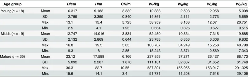
After being transported to the laboratory, the subsamples were oven-dried at 85°C until a constant weight was obtained. Dry weights were computed for all tree components using the ratio of dry weight to fresh weight from subsamples from each component and multiplied by their known fresh weights. The total tree biomass was generated by summing the biomass of each component. The statistics of the tree variables and the biomass of each component at dif-ferent age groups are listed inTable 1.
Tree biomass model
demonstrated that the allometric relationships changed, even within the lifetime of individuals of a single species. Here, we used the following six equations to estimate the tree component biomass according to three age groups, including young, middle-aged, and mature forests.
W¼aDb ð1Þ
W¼aDbHc ð2Þ
W ¼aDbCRc ð3Þ
W ¼aðD2HÞb ð4Þ
W¼aðD2HÞbCRc ð5Þ
W¼aDbHcCRd ð6Þ
whereWis tree biomass in kg, andα,b,c, anddare the parameters to be estimated. Overman
et al. [39] reported that it is convenient to use logarithms for thefitting model and for dealing with heteroscedasticity. Therefore, Eqs (1) to (6) can be linearized using logarithms in the fol-lowing equations, respectively:
lnðWÞ ¼aþblnðDÞ ð7Þ
lnðWÞ ¼aþblnðDÞ þclnðHÞ ð8Þ
lnðWÞ ¼aþblnðDÞ þclnðCRÞ ð9Þ
lnðWÞ ¼aþblnðD2HÞ ð10Þ
Table 1. Tree variables and biomass of each component ofC.equisetifoliain different age groups.
Age group D/cm H/m CR/m WT/kg WB/kg WL/kg WR/kg
Young(n= 18) Mean 6.317 9.183 3.332 12.388 2.593 2.958 5.008
SD. 2.759 3.359 0.840 14.861 2.111 2.773 5.669
Max. 13.1 15.4 5.725 58.959 8.163 12.07 20.751
Min. 2.5 4.1 1.95 0.664 0.326 0.627 0.515
Middle(n= 19) Mean 12.747 14.016 3.834 52.450 10.534 7.315 19.885
SD. 2.132 2.869 0.644 23.788 6.853 3.308 9.832
Max. 16.8 19.5 5.05 103.707 34.249 15.258 40.798
Min. 9.3 8 2.85 18.243 3.871 2.569 7.343
Mature (n= 35) Mean 23.12 17.589 6.166 237.858 37.271 26.427 88.173
SD. 5.092 2.207 1.876 111.181 32.687 31.652 61.748
Max. 36.3 22.7 10.55 537.391 155.955 153.917 291.325
Min. 15.6 14.1 3.4 91.731 11.208 7.618 29.106
Note:Dis the diameter at breast height;His the total tree height;CRis the crown radius;Wtis the biomass of the trunk;WBis the biomass of the branch;
WLis the biomass of the leaf;WRis the biomass of the root; SD is the standard deviation.
lnðWÞ ¼aþblnðD2HÞ þclnðCRÞ ð11Þ
lnðWÞ ¼aþblnðDÞ þclnðHÞ þdlnðCRÞ ð12Þ
wherea= ln(α). The log-transformation of the data leads to a biased biomass estimation [40,
41], and uncorrected biomass estimates are theoretically expected to generate a systematic underestimation. The bias is not an arithmetic constant value but rather a constant proportion of the estimation [42]. Baskerville [43] recognized this detail and gave a multiplicative correc-tion factor for this bias:
CF¼expðs
2
2Þ ð13Þ
wheres2¼
X
ðlnW lnW^Þ2
=ðn 2Þis the mean square error from the logarithmic regres-sion, andnis the sample size. Therefore, the estimated tree biomass (W^) could be calculated fromEq (14):
^
W ¼expðln^WÞCF ð14Þ
Model selection
The coefficient of determination (R2) is the most widely used criterion in biomass model lit-erature. However, in many situations, it has been used uncritically. The R2is deceptive because it increases with the addition of polynomial terms and with the inclusion of new pre-dictors [44,45]. Therefore, R2can sometimes be a poor estimator of model performance. The mean absolute prediction error (MAPE) [33,46,47] was used as the primary metric to evalu-ate and compare the performance of models, whose statistical properties are well known and commonly used in forecasting and model comparison in ecology and environment assess-ment.
R2¼1
SðWi W^iÞ 2=
SðWi WÞ
2 ð15Þ
MAPE¼1
n
Xn
i¼1
jWi W^ij Wi
ð16Þ
whereWi= observed biomass value treei, andW^iandW = the estimated value and the aver-age, respectively, ofWi.
In this study, we first used the above Eqs (7–12) andEq (14)to estimate the biomass of tree components, including the trunk, the branch, the leaf and the root, by age groups. Then, we selected the best equation according to the evaluation statistics (R2and MAPE) and the signifi-cance of the estimated parameters. Finally, the best equation for each component was fitted as a system of equations ensuringWTotal=WT+WB+WL+WRusing a seemingly unrelated
regression (SUR) [48]:
lnðWTÞ ¼fðD;H;CRÞ lnðWBÞ ¼fðD;H;CRÞ lnðWLÞ ¼fðD;H;CRÞ lnðWRÞ ¼fðD;H;CRÞ
whereCFT,CFB,CFL,CFRare the correction factors for trunk biomass, branch biomass, leaf
bio-mass, and root biomass by age groups, respectively. Thefitting procedure involved the use of option SUR of the procedure MODEL in SAS. The normality of the residual for total biomass pre-diction (W^Total) was tested using the normal Q-Q plot and the Shapiro-Wilk test of normality.
Results
Biomass allocation
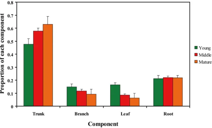
The tree biomass ofC.equisetifoliaover the three age groups was highest in the trunk, followed by (in decreasing order) the root, the branch, and the leaf. The proportion of the biomass from trunk increased with forest age, while that in the branch and the leaf declined, especially for the leaf, which significantly declined from the young forest to the middle-aged forest (ANOVA analysis,F= 30.457,P<0.001). In addition, the proportion of biomass ofC.equisetifoliathat from the root was independent of tree age (ANOVA analysis,F= 0.276,P= 0.76). Of the total biomass, the trunk accounted for 47.6% to 62.9% from the young forest to the mature forest, respectively, the branch for 14.9% to 9.2%, the leaf for 16.4% to 6.2%, and the root for 21.1% to 21.7% (S1 Table,Fig 1).
Each component biomass model selection by age groups
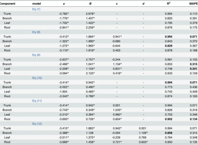
We developed the tree component biomass models for young, middle-aged and mature forests using Eqs (7–12), and the correction factor was applied to back-transformed predictions (Eq 14). The R2and the MAPE were calculated based on the back-transformed predictions.
Fig 1. Proportion of the tree biomass from the trunk, the branch, the leaf, and the root in young, middle-aged, and mature forests.
In the young forest, both Eqs8and10performed the best in estimating the trunk biomass compared to other models in terms of the MAPE, the R2, and the parameter significance. Both of these equations explained 99.4% of the variance in the trunk biomass, and the MAPE was 0.071 (Table 2). Here we used theEq 8to model the trunk biomass. The best model for estimat-ing the branch biomass wasEq 9compared to other models in terms of the MAPE and parame-ter significance. The second performance modelEq 11resulted in a 1.26% increase in the MAPE over the best model (Eq 9). The best model introducing the variableCRexplained 85.3% of the variance in the branch biomass. Although the MAPE inEq 12was equal toEq 9, the two-parameter estimates of this model were not significant at a level of 0.05. In terms of the MAPE and the parameter estimate significance, the best model for estimating the leaf biomass wasEq 9, in which the MAPE was 0.341, lower than that of the other models. For the root
Table 2. Parameter estimates and model evaluation statistics of each biomass model for the young forest.
Component model a B c d R2 MAPE
Eq (7)
Trunk -2.785* 2.678* - - 0.994 0.110
Branch -1.776* 1.407* - - 0.820 0.391
Leaf -1.702* 1.422* - - 0.795 0.379
Root -2.841* 2.259* - - 0.876 0.175
Eq (8)
Trunk -3.413* 1.884* 0.941* - 0.994 0.071
Branch -1.322* 1.980* -0.680 - 0.843 0.372
Leaf -1.272* 1.965* -0.644 - 0.829 0.367
Root -3.110* 1.919* 0.403 - 0.878 0.168
Eq (9)
Trunk -2.637* 2.757* -0.244 - 0.991 0.103
Branch -2.466* 1.041* 1.134* - 0.853 0.315
Leaf -2.208* 1.154* 0.831* - 0.746 0.341
Root -3.094* 2.125* 0.416* - 0.933 0.159
Eq (10)
Trunk -3.414* 0.942* - - 0.994 0.071
Branch -2.022* 0.480* - - 0.773 0.436
Leaf -1.954 0.485* - - 0.742 0.409
Root -3.343* 0.789* - - 0.874 0.163
Eq (11)
Trunk -3.414* 0.942* 0.001 - 0.994 0.071
Branch -2.743* 0.349* 1.245* - 0.826 0.319
Leaf -2.510* 0.384* 0.960* - 0.703 0.348
Root -3.693* 0.726* 0.604* - 0.952 0.134
Eq (12)
Trunk -3.415* 1.883* 0.942* 0.001 0.994 0.071
Branch -2.388* 1.128 -0.094 1.109* 0.858 0.315
Leaf -2.011* 1.375* -0.239 0.769 0.764 0.348
Root -3.689* 1.456* 0.721* 0.603* 0.950 0.135
Note: Values in bold denote the best statistic among six biomass models for each component.
*means significant at 0.05 level.
biomass model,Eq 11with the variablesD2HandCRwas the best model, as the MAPE was the lowest, and the R2was the highest. In addition, the three parameters of this model were all sig-nificant at a level of 0.05.
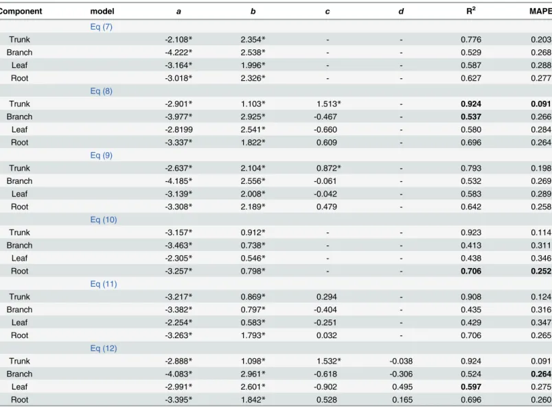
In the middle-aged forest,Eq 8explained 92.4% of the variance in the trunk biomass (Table 3). In addition, the MAPE was lowest, 55.2% lower than that of the equation with only
D(Eq 7), indicating that the total tree height greatly improved the trunk biomass model. For the branch biomass model, although the MAPE fromEq 12was the lowest, the parameters of
HandCRwere not significant at a level of 0.05.Eq 7was the best for estimating the branch bio-mass and the leaf biobio-mass. In terms of the root biobio-mass, both the MAPE and the R2showed thatEq 10was the best model.
Table 3. Parameter estimates and model evaluation statistics of each biomass model for the middle-aged forest.
Component model a b c d R2 MAPE
Eq (7)
Trunk -2.108* 2.354* - - 0.776 0.203
Branch -4.222* 2.538* - - 0.529 0.268
Leaf -3.164* 1.996* - - 0.587 0.288
Root -3.018* 2.326* - - 0.627 0.277
Eq (8)
Trunk -2.901* 1.103* 1.513* - 0.924 0.091
Branch -3.977* 2.925* -0.467 - 0.537 0.266
Leaf -2.8199 2.541* -0.660 - 0.580 0.284
Root -3.337* 1.822* 0.609 - 0.696 0.264
Eq (9)
Trunk -2.637* 2.104* 0.872* - 0.793 0.198
Branch -4.185* 2.556* -0.061 - 0.532 0.269
Leaf -3.139* 2.008* -0.042 - 0.583 0.289
Root -3.308* 2.189* 0.479 - 0.642 0.258
Eq (10)
Trunk -3.157* 0.912* - - 0.923 0.114
Branch -3.463* 0.738* - - 0.413 0.311
Leaf -2.305* 0.546* - - 0.438 0.346
Root -3.257* 0.798* - - 0.706 0.252
Eq (11)
Trunk -3.217* 0.869* 0.294 - 0.908 0.124
Branch -3.382* 0.797* -0.404 - 0.435 0.316
Leaf -2.254* 0.583* -0.251 - 0.429 0.347
Root -3.263* 1.793* 0.032 - 0.706 0.265
Eq (12)
Trunk -2.888* 1.098* 1.532* -0.038 0.924 0.091
Branch -4.083* 2.961* -0.618 -0.306 0.524 0.264
Leaf -2.991* 2.601* -0.902 0.495 0.597 0.275
Root -3.395* 1.842* 0.528 0.165 0.696 0.260
Note: Values in bold denote the best statistic among six biomass models for each component.
*means significant at 0.05 level.
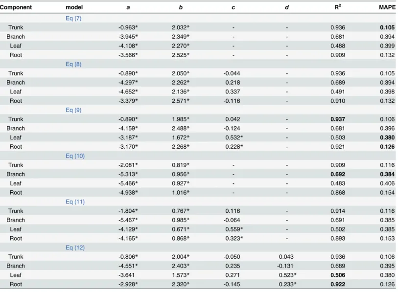
In mature forests,Eq 7with onlyDwas best in terms of having the lowest MAPE and the second highest R2(Table 4). Although the MAPE values from Eqs7and8were equal, the effect ofHon the trunk biomass was not significant for this dataset (P>0.05). The best equation for estimating the branch biomass wasEq 10compared to other models in terms of the MAPE and the R2.Eq 9with variablesDandCRhad the lowest MAPE compared to the other models in estimating the biomass of the leaf and the root. In terms of leaf biomass, addingCRgreatly improved estimates, increasing the R2and reducing the MAPE compared to the equivalent equation withoutCR(Eq 7).
Table 4. Parameter estimates and model evaluation statistics of each biomass model for the mature forest.
Component model a b c d R2 MAPE
Eq (7)
Trunk -0.963* 2.032* - - 0.936 0.105
Branch -3.945* 2.349* - - 0.681 0.394
Leaf -4.108* 2.270* - - 0.488 0.399
Root -3.566* 2.525* - - 0.909 0.132
Eq (8)
Trunk -0.890* 2.050* -0.044 - 0.936 0.105
Branch -4.297* 2.262* 0.218 - 0.689 0.394
Leaf -4.652* 2.136* 0.337 - 0.491 0.398
Root -3.379* 2.571* -0.116 - 0.910 0.132
Eq (9)
Trunk -0.890* 1.985* 0.042 - 0.937 0.106
Branch -4.159* 2.488* -0.124 - 0.681 0.396
Leaf -3.187* 1.672* 0.532* - 0.503 0.380
Root -3.170* 2.268* 0.228* - 0.921 0.126
Eq (10)
Trunk -2.081* 0.819* - - 0.909 0.116
Branch -5.313* 0.956* - - 0.692 0.384
Leaf -5.466* 0.927* - - 0.483 0.406
Root -4.938* 1.016* - - 0.868 0.154
Eq (11)
Trunk -1.804* 0.767* 0.116 - 0.914 0.116
Branch -5.467* 0.985* -0.064 - 0.691 0.385
Leaf -4.129* 0.671* 0.559* - 0.502 0.385
Root -4.165* 0.868* 0.323* - 0.893 0.153
Eq (12)
Trunk -0.806* 2.004* -0.050 0.043 0.936 0.106
Branch -4.551* 2.403* 0.235 -0.131 0.689 0.395
Leaf -3.641 1.573* 0.271 0.523* 0.506 0.380
Root -2.928* 2.320* -0.145 0.233* 0.922 0.126
Note: Values in bold denote the best statistic among six biomass models for each component.
*means significant at 0.05 level.
Biomass predictions using SUR method by age groups
Based on the best model for each component analyzed above, we used SUR method to estimate a system of equations (Eq (15)) to ensure the additivity of the total tree biomass, including the trunk biomass, the branch biomass, the leaf biomass, and the root biomass.
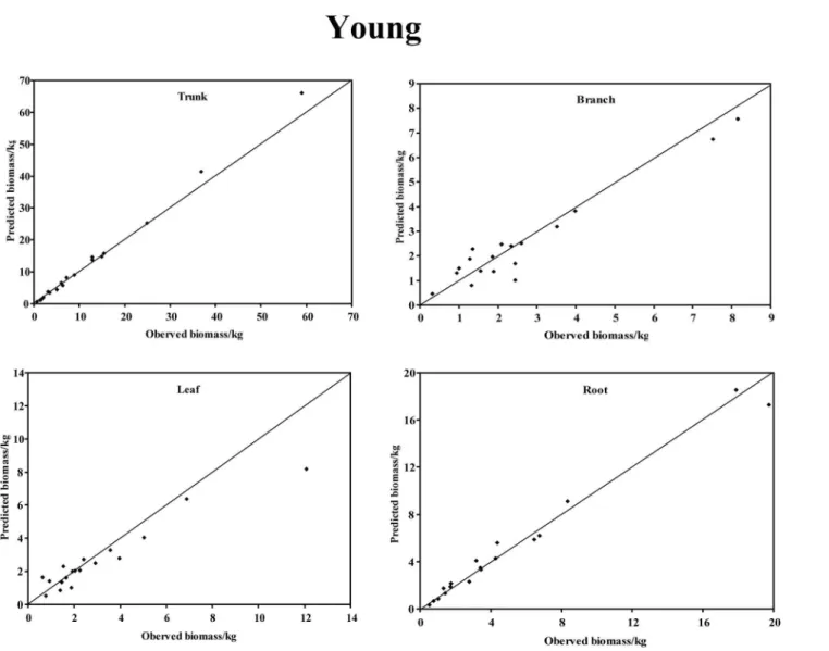
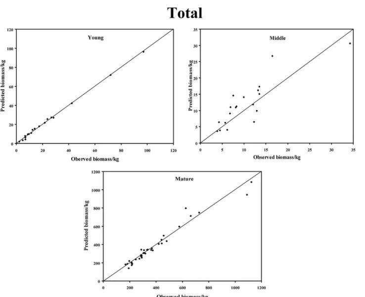
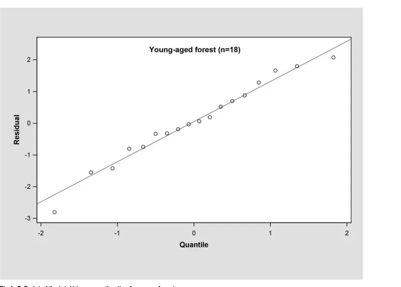
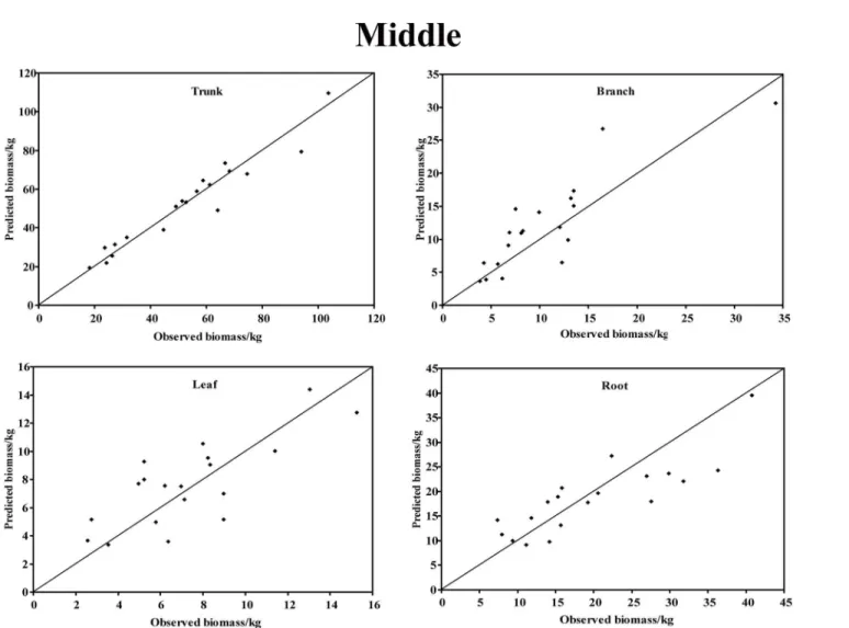
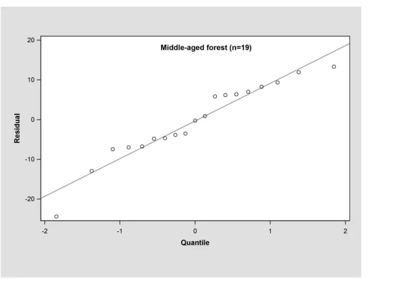
In the young forest, the trunk biomass predictions were close to the observed biomass, as well as the branch biomass, leaf biomass and root biomass (Fig 2). In terms of the total bio-mass predictions, the predictions were highly correlated with the observed values (Fig 3), and the residual was normal (Fig 4, Shapiro-Wilk test,P= 0.891>0.05). In the middle-aged forest, the fit accuracy of the trunk biomass was very high (Fig 5). However, the branch bio-mass, leaf biomass and root biomass prediction performed worse than the trunk biomass (Fig 5). In addition, the total biomass predictions were very close to observed values (Fig 3), and the residual for total biomass predictions was also normal (Fig 6, Shapiro-Wilk test,
P= 0.274>0.05). The SUR method also showed good performance on predicting the trunk
Fig 2. The relationship between the predicted biomass and observed biomass for four components in young forest.
biomass, branch biomass, leaf biomass, root biomass in the mature forest (Fig 7), as well as the total biomass which could be depicted by the relationship and residual plots (Shapiro-Wilk test,P= 0.839>0.05, Figs3and8). All the parameter estimates of the selected biomass models by age groups using SUR method are displayed inTable 5.
Discussion
Variation in the tree biomass and its allocation to components was commonly found in com-parisons among individuals, ages, stands, regions, and species [49–51]. In the study, the pro-portion of trunk biomass to total tree biomass significantly increased at a level of 0.05 in the young forest to the mature forest and represented the greatest portion of the total biomass, which also could be found in other studies [52–53]. However, the proportion of branch bio-mass and leaf biobio-mass decreased from the young forest to the mature forest. The result is
Fig 3. The relationship between the predicted biomass and observed biomass for total biomass in young, middle-aged, and mature forests.
consistent with findings of Scots pine (Pinus sylvestris) [54] and loblolly pine (Pinus taeda) [55]. The leaf biomass is a valuable component to quantify because it is highly correlated with forest productivity in young forests, which typically peak as canopies close and then decreases with stand age [56–57]. The relative amount of biomass from the leaf in this study significantly decreased from the young forest to the middle-aged forest (Fig 1). The individual-tree root bio-mass increases with tree age to maintain a balance between the above- and belowground com-ponents [58–59]. Although the root biomass increased with tree age, the proportion of root biomass to the total tree remained stable at the three stages, indicating that roots are a crucial component when considering biomass partitioning forC.equisetifolia. Bijaket al. [60] reported a decrease in the proportion of root biomass in relation to total biomass of the silver birch (Betula pendula) with the increasing tree age, which was different in this study.C.equisetifolia
has a strong root system to be adaptable to degraded sites, which results in a high proportion of biomass allocation at the whole stand development stages.
The main predictor of biomass,D, tends to work quite well for predicting tree biomass [61–
63], but it fails to provide accurate estimates of biomass component fractions [64]. Many stud-ies have shown that improvements can be made by adding variables other thenDto improve
Fig 4. Q-Q plot of the total biomass estimation for young forest.
tree biomass estimation. The most widely used variable is the total tree height because height-diameter relationships vary across a range of ecological conditions [65–67]. Chave et al. [68] found that the inclusion of height reduced the standard error of aboveground biomass esti-mates from 19.2 to 12.5% in predicting the biomass of tropical forests. As noted above, more than 50% of the aboveground biomass was from the trunk. In the trunk biomass models of this study, the MAPE from equation with variableHwas 35.45% and 55.17% lower than that of the equation with only the variableDin the young and middle-aged forests, respectively. In the leaf biomass equations, other variables, such as tree age, crown competition factors [69] that are closely related to the leaf area, crown volume and canopy dynamics, are often not included for individual trees. For realistic predictions of the leaf biomass, variables other thanHmust be included [70–72]. The treeCRis a useful indicator of vigor and stand density [73–75]. Mea-surements of crown dimensions have been recently emphasized as important to improving tree biomass estimation, including measurements of the crown length, the crown width and the diameter of the largest branch in a tree [29,33]. Wanget al. [76] demonstrated that crown width is an important determinant of leaf biomass for Korean pine (Pinus koraiensis). We also
Fig 5. The relationship between the predicted biomass and observed biomass for four components in middle-aged forest.
found that equations with the variableCRgreatly improved root biomass estimates (Tables2
and4). However, some studies reported that root biomass equations were not improved by including crown width [77–78]. In addition, tree age is the other factor. Disregarding tree age may give biased biomass estimates [79]. In this study, we developed a biomass model for each tree component by age group, which could be of benefit for forest managers when evaluating biomass storage and carbon sequestration forC.equisetifoliain the tropical forest of Hainan Island.
When we estimate biomass from tree components, it is desirable to have the property of additivity in the biomass estimations of the components. The principle of additivity in which the biomass estimations from component equations added to the total biomass has long been recognized [16]. Parresol [48] found that a seemingly unrelated regression (SUR) method can be applied when considering the contemporaneous correlations among different components and biomass additivity, including the trunk, the branch, the leaf, and the root, from the same tree. The SUR method led to efficient parameter estimates by considering inherent correlations among biomass components. Russell [80] reported that the largest gain in using the SUR method is that confidence and prediction intervals for biomass estimates are narrower than
Fig 6. Q-Q plot of total biomass estimation for middle-aged forest.
isolated estimates. In this study, based on the best individual regressions for each component independently in young, middle-aged and mature forests, the systems of equations presented herein will provide reasonable estimates for those who wish to estimate the biomass ofC. equi-setifoliatrees in the tropical forest of Hainan Island (Figs2–7).
Conclusion
The tree biomass ofC.equisetifoliaover the young, middle and mature three age groups in a tropical forest of Hainan Island was highest in the trunk, followed by (in decreasing order) the root, the branch, and the leaf. The biomass from the trunk increased with forest age, while that in the branch and the leaf declined, especially for the leaf. In this study, 12 equations for bio-mass components by three age groups were established and the best models for estimating tree biomass components were selected according to the R2and MAPE. Among these 12 equations, only three equations with variableDwere made, while the remaining equations introduced the other variables, includingH,D2H, andCR. An equation including theCRgreatly improved the model performance and reduced the error, especially for the young and mature forests. Also
Fig 7. The relationship between the predicted biomass and observed biomass for four components in mature forest.
Table 5. Parameter estimates of the selected models for different components by age groups using SUR method.
Component Age groups a b c
Young
Trunk -3.599 2.274 0.709
Branch -2.436 1.123 0.953
Leaf -2.158 1.211 0.640
Root -3.983 0.771 0.625
Middle
Trunk -2.822 1.218 1.375
Branch -6.197 3.358
-Leaf -4.247 2.450
-Root -2.620 0.712
-Mature
Trunk -1.211 2.109
-Branch -5.127 0.935
-Leaf -2.704 1.827
-Root -5.487 2.820 0.534
Note: In young forest, trunk: ln(W) =a+bln(D) +cln(H); branch and leaf: ln(W) =a+bln(D) +cln(CR); root: ln(W) =a+bln(D2H) +cln(CR). In
middle-aged forest, trunk: ln(W) =a+bln(D) +cln(H); branch and leaf: ln(W) =a+bln(D); root: ln(W) =a+bln(D2H). In mature forest, trunk and leaf: ln(W) =a+
bln(D); branch: ln(W) =a+bln(D2H); root: ln(W) =a+bln(D) +cln(CR).
taking into account the biomass additivity, our findings suggest that the seemingly unrelated regression (SUR) not only gave efficient and accurate estimates but also achieved the logical additivity of biomass forC.equisetifoliain a tropical forest of Hainan Island.
Supporting Information
S1 Table. Proportion of tree biomass from components in young, middle-aged, and mature forests.
(DOC)
Author Contributions
Conceived and designed the experiments: YX ZY. Performed the experiments: YX XW ZL DL SS. Analyzed the data: YX ZL. Contributed reagents/materials/analysis tools: YX DL. Wrote the paper: YX.
References
1. Sanquetta CR, Behling AB, Corte APD, Netto SP, Schikowski AB, do Amaral M. Simultaneous estima-tion as alternative to independent modeling of tree biomass. Ann For Sci. 2015; 1–14.
2. Fahey TJ, Woodbury PB, Battles JJ, Goodale CL, Hamburg SP, Ollinger SV, et al. Forest carbon stor-age: Ecology, management, and policy. Front. Ecol. Environ. 2010; 8: 245–252.
3. West GB, Brown JH, Enquist BJ. A general model for the origin of allometric scaling laws in biology. Sci-ence 1997; 276:122–126. PMID:9082983
4. Parresol BR. Assessing tree and stand biomass: a review with examples and, critical comparisons. For Sci. 1999; 45(4):573–593.
5. Basuki TM, van Laake PE, Skidmore AK, Hussin TA. Allometric equations for estimating the above-ground biomass in tropical lowland Dipterocarp forests. For Ecol Manage. 2009; 257: 1684–1694. 6. Zhang X, Duan A, Zhang J. Tree biomass estimation of Chinese fir (Cunninghamia lanceolata) based
on Bayesian method. PLoS ONE 2013; 8(11): e79868. doi:10.1371/journal.pone.0079868PMID: 24278198
7. Zhou G. Wang Y, Jiang Y, Yang Z. Estimating biomass and net primary production from forest inventory data: a case study of China’sLarixforests. For Ecol Manage. 2002; 169: 149–157.
8. Pan Y, Luo T, Birdsey R, Hom j, Melillo J. New estimates of carbon storage and sequestration in Chi-na’S forests: effects of age-class and method on inventory-based carbon estimation. Climatic Change. 2004; 67(2): 211–236.
9. Schroeder P, Brown S, Mo J, Bridsey R, Cieszewski C. Biomass estimation for temperate broadleaf for-ests of the United States using inventory data. For Sci. 1997; 43: 424–434.
10. Fang J, Chen A, Peng C, Zhao S, Ci L. Changes in forest biomass carbon storage in China between 1949 and 1998. Science 2001; 291: 2320–2322.
11. Jalkanen A, Makippaa r, Stahl G, Lehtonen A, Petersson H. Estimation of the biomass stock of trees in Sweden: comparison of biomass equations and age-dependent biomass expansion factors. Ann For Sci. 2005; 62: 845–851.
12. Levy PE, Hale SE Nicoll BC. Biomass expansion factors and root: shoot rations for coniferous tree spe-cies in Great Britain. Forestry 2004; 77: 421–430.
13. Petersson H, Holm S, Stahl G, Alger D, Fridman J, Lehtonen A, et al. Individual tree biomass equations or biomass expansion factors for assessment of carbon stock changes in living biomass-A comparative study. For Ecol Manage. 2012; 270: 78–84.
14. Wang X, Fang J, Zhu B. Forest biomass and root-shoot allocation in northeast China. For Ecol Manage. 2008; 255: 4007–4020.
15. Nogueira EM, Fearnside PM, Nelson BW. Normalization of wood density in biomass estimates of Ama-zon forests. For Ecol Manage. 2008; 256: 990–996.
16. Kozak A. Methods for ensuring additivity of biomass components by regression analysis. For Chron. 1970; 46: 402–404.
18. Zhang X, Lei Y, Cao QV. Compatibility of stand basal area predictions based on forecast combination. For Sci. 2010; 56: 552–557.
19. Mendonza LA. Growth and uses ofCasuarina cunninghamianain Argentina. In: Midgley SJ, Turnbull JW, Johnston RD (eds)CasuarinaEcology. Management and Utilization, CSIRO, Canberra, 1983; 53–54. 20. Yang JC, Chang TR, Chen TH, Chen ZZ. Provenance trial ofCasuarina equisetifoliain Taiwan I. Seed
weight and seedling growth. Bulletin of Taiwan Forestry Research Institute 1995; 10: 195–207. 21. Zhong C, Bai J, Zhang Y. Introduction and conservation of Casuarina trees in China. For Res. 2005;
18: 345–350. (in Chinese)
22. Ye G. Coastal Ecosystem ofCasuarinaPlantation. Chinese Forestry Publishing House, Beijing, 2011. (in Chinese)
23. Liu X, Lu Y, Xue Y, Zhang X. Testing the importance of native plants in facilitation the restoration of coastal plant communities dominated by exotics. For Ecol Manage. 2014; 322: 19–26.
24. Wu C, Wang X, Xue Y, Wang X, Lin Z. Clonal ofCasuarina equisetifoliaroot biomass and its estimation model in northeastern Hainan. J NE For Univer. 2014; 42: 67–71. (in Chinese)
25. Wang FM, Xu X, Zou B, Guo ZH, Li ZA, Zhu WX. Biomass accumulation and carbon sequestration in four different agedCasuarina equisetifoliacoastal shelterbelt plantations in south China. PLoS ONE 2013; 8: e77449. doi:10.1371/journal.pone.0077449PMID:24143236
26. Lie G, Xue L. Biomass allocation patterns in forests growing different climatic zones of China. Trees 2015; 1–8.
27. Yang Z, Xue Y, Liu X, Wang X, Lin Z. Additivity in tree biomass models ofCasuarina equisetifoliain Hai-nan Province. J NE For Univer. 2015; 43: 36–40. (in Chinese)
28. Leites LP, Robinson AP, Crookston NL. Accuracy and equivalence testing of crown ratio models and assessment of their impact on diameter growth and basal area increment predictions of two variants of the forest vegetation simulator. Can J For Res. 2009; 39: 655–665.
29. Goodman RC, Phillips OL, Baker TR. The importance of crown dimensions to improve tropical tree bio-mass estimates. Ecol Appl. 2014; 24: 680–698. PMID:24988768
30. Levy PE, Hale SE, Nicoll BC. Biomass expansion factors and root: shoot ratios for coniferous tree spe-cies in Great Britain. Forestry 2004; 77(5): 421–430
31. Soethe N, Lehmann J, Engels C. Root tapering between branching points should be included in fractal root system analysis. Ecol Model. 2007; 207: 363–366
32. Mugasha WA, Eid T, Bollandsås OM, Malimbwi RE, Chamshama SAO, Zahabu E et al. Allometric mod-els for prediction of above- and belowground biomass of trees in the miombo woodlands of Tanzania. For Ecol Manage. 2013; 310: 87–101.
33. MacFarlane DW. A generalized tree component biomass model derived from priciples of variable allometry. For Ecol Manage. 2015; 354: 43–55.
34. Cannell MGR. Woody biomass of forest stands. For Ecol Manage. 1984; 8: 299–312.
35. Chave J, Andalo C, Brown S, Cairns MA, Chambers JQ, Eamus D, et al. Tree allometry and improved esti-mation of carbon stocks and balance in tropical forests. Oecologia 2005; 145: 87–99. PMID:15971085 36. Iida Y, Poorter L, Sterck FJ, Kassim AR, Kubo T, Potts MD, et al. Wood density explains architectural
differentiation across 145 co-occurring tropical tree species. Functional Ecology 2012; 26: 274–282. 37. Huxley JS, Tessier G. Terminology of relative growth. Nature 1936; 137: 780–781.
38. Niklas KJ. Size-dependent allometry of tree height, diameter and trunk taper. Ann Bot. 1995; 75: 217–
227.
39. Overman JPM, Witte HJL, Saldarriaga JG. Evaluation of regression models for above-ground biomass determination in Amazon rainforest. J Trop Ecol 1994; 10: 207–218.
40. Snowdon P. A ratio estimator for bias correction in logarithmic regressions. Can J For Res. 1991; 21: 720–724.
41. Medhurst JL, Battaglia M, Cherry ML, Hunt MA, White DA, Beadle CL. Allometric relationships for Euca-lyptus nitens(Deane and Maiden) Maiden plantations. Trees 1999; 14: 91–101.
42. Wiant HV, Harner EJ. Percent bias and standard error in logarithmic regression. For Sci. 1979; 20: 167–168.
43. Baskerville GL. Use of logarithmic regression in the estimation of plant biomass. Can J For Res. 1972; 2: 49–53.
45. Mbow C, Verstraete MM, Sambou B, Diaw AT, Neufeldt H. Allometric models for aboveground biomass in dry savanna trees of the Sudan and Sudan-Guinean ecosystems of Southern Senegal. J. For. Res. 2013; 19: 340–347.
46. Yao X, Fu B, Lu Y, Sun F, Wang S. Liu M. 2013. Comparison of four spatial interpolation methods for estimating soil moisture in a complex terrain catchment. PLoS ONE 2013; 8 (1): e54660. doi:10.1371/ journal.pone.0054660PMID:23372749
47. Sileshi GW. 2014. A critical review of forest biomass estimation models, common mistakes and correc-tive measures. For Ecol Manage. 2014; 329: 237–254.
48. Parresol BR. Additivity of nonlinear biomass equations. Can J For Res. 2001; 31: 865–878.
49. Canham CD, Berkowitz AR, Kelly VR, Lovett GM, Ollinger SV, Schnurr J. Biomass allocation and multi-ple resource limitation in tree seedlings. Can J For Res. 1996; 26: 1521–1530.
50. Li X, Yi M, Son Y, Park PS, Lee KH, Son YM, et al. Biomass and carbon storage in an age-sequence of Korean Pine (Pinus koraiensis) plantation forests in central Korea. J. Plant Biol. 2011; 54: 33–42. 51. Wang J, Fan J, Fan X, Zhang C, Wu L, Gadow KV. Crown and root biomass equations for the small
trees ofPinus koraiensisunder canopy. Dendrobiology 2013; 70: 13–25.
52. Gower ST, Pongracic S, Landsberg JL. A global trend in belowground carbon allocation: can we use the relationship at smaller scales? Ecology 1996; 77(6): 1750–1755.
53. Peichl M, Arain A. Allometry and partitioning of above-and belowground tree biomass in an aged-sequence of white pine forests. For Ecol Manage. 2007; 253: 68–80.
54. Vaninen P, Ylitalo H, Sievänen R, Mäkelä A. Effects of age and site quality on the distribution of bio-mass in Scots pine (Pinus sylvestrisL.). Trees 1996; 10: 231–238.
55. Albaugh TJ, Allen HL, Dougherty PM, Johnsen KH. Long term growth responses of loblolly pine to opti-mal nutrient and water resource availability. For Ecol Manag. 2004; 192: 3–19.
56. Ryan MG, Binkley D, Fownes JH. Age-related decline in forest productivity: pattern and process. Adv Ecol Res. 1997; 27: 211–262.
57. Burkes EC, Will RE, Barron-Gafford GA, Teskey RO, Shiver B. Biomass partitioning and growth effi-ciency of intensively managedPinus taedaandPinus elliottiistands of different planting densities. For Sci. 2003; 4: 224–234.
58. Waring RH, Pitman GB. Modifying lodgepole pine stands to change susceptibility to mountain pine-bee-tle attack. Ecology 1985; 66: 889–897.
59. Van Lear DH, Kapeluck PR. Above and below-stump biomass and nutrient content of a mature loblolly pine plantation. Can. J. For. Res. 1995; 25: 361–367.
60. Bijak SZ, Zasada M, Bronisz A, Bronisz K, Czajkowski M, Ludwisiak L, et al. Estimating coarse roots biomass in young silver birch stands on post-agricultural lands in central Poland. Silva Fennica 2013; 47: 1–14.
61. van Laar A. Sampling for above-ground biomass forPinus radiatain theBosboukloof catchmentat Johnkershoek. South Afr For J. 1982; 123: 8–13.
62. Bi H, Turner J, Lambert MJ. Additive biomass equations for native eucalypt forest trees of temperate Australia. Trees 2004; 18: 467–479.
63. Case BS, Hall RJ. Assessing prediction errors of generalized tree biomass and volume equations for the boreal forest region of west-central Canada. Can J For Res. 2008; 38: 878–889.
64. Jenkins JC, Chojnacky DC, Heath LS, Birdsey RA. National scale biomass estimators for United States tree species. For Sci. 2003; 49: 12–35.
65. Ketterings QM, Coe R, van Noordwijk M, Ambagau Y, Palm CA. Reducing uncertainty in the use of allo-metric biomass equations for predicting aboveground tree biomass in mixed secondary forests. For Ecol Manage. 2001; 146: 199–209.
66. Feldpausch TR, Lloyd J, Lewis SL, Brienen RJW, Gloor M, Mendoza AM, et al., 2012. Tree height inte-grated into pantropical forest biomass estimates. Biogeosciences 2012; 9: 3381–3403.
67. Zhang X, Duan A, Zhang J, Xiang C. Estimating tree height-diameter models with the Bayesian method. Sci World J. 2014; 683691: 1–9.
68. Chave J, Andalo C, Brown S, Cairns MA, Chambers JQ, Eamus D. Tree allometry and improved esti-mation of carbon stocks and balance in tropical forests. Oecologia, 2005; 145: 87–99. PMID: 15971085
70. Saint-André L, Thongo M’Bou A, Mabiala A, Mouvondy WJ, Jourdan C, Roupsard O, et al. Age-related equations for above and below-ground biomass of a Eucalyptus hybrid in Congo. For. Ecol. Manage. 2005; 205, 199–214.
71. Tobin B, Black K, Osborne B, Reidy B, Bolger T, Nieuwenhuis M. Assessment of allometric algorithms for estimating leaf biomass. Leaf area index and litter fall in different aged sitka spruce forests. Forestry 2006; 79: 453–465.
72. António N, Tomé M, Tomé J, Soares P, Fontes L. Effect of tree, stand, and site variables on the allome-try of Eucalyptus globulus tree biomass. Can. J. For. Res. 2007; 37: 895–906.
73. Hasenauer H, Monserud RA. A crown ratio model for Austrian forests. For Ecol Manage. 1996; 84: 49–60. 74. Popoola FS, Adesoye PO. Crown ratio models for tectonaģrandis (Linn. f) stands in Osho forest
reserve, Oyo state, Niġeria. J For Sci. 2012; 28(2): 63–67.
75. Clutter JL, Fotson JC, Pienaar LV, Brister GH, Bailey RL. Timber Management: A Quantitative Approach. John Wiley and sons, New York. 1983.
76. Wang J, Fan J, Fan X, Zhang C, Wu L, Gadow KV. Crown and root biomass equations for the small trees ofPinus koraiensisunder canopy. Dendrobiology 2013; 70: 13–25.
77. Wagner RG, Ter-Mikaelian MT. Comparison of biomass component equations for four species of north-ern coniferous tree seedlings. Ann For Sci. 1999; 56 (3): 193–199.
78. Wang F, Xu X, Zou B, Guo Z, Li Z, Zhu W. (2013) Biomass accumulation and carbon sequestration in four different agedCasuarina equisetifoliacoastal shelterbelt plantations in south China. PLoS ONE 2013: 8(10): e77449. doi:10.1371/journal.pone.0077449PMID:24143236
79. Mäkelä A, Valentine HT. Crown ratio influences allometric scaling in trees. Ecology 2006; 87 (12): 2967–2972. PMID:17249219