INDIVIDUAL BIOVOLUME OF SOME DOMINANT COPEPOD SPECIES IN
COASTAL WATERS OFF BUENOS AIRES PROVINCE, ARGENTINE SEA
María Delia Viñas 1,2,3,*, Nadia Rosalía Diovisalvi 3,4 and Georgina Daniela Cepeda 1,2,3
1Instituto Nacional de Investigación y Desarrollo Pesquero (INIDEP) (Paseo Victoria Ocampo Nº 1, B7602HSA, Mar del Plata, Argentina)
2
Consejo Nacional de Investigaciones Científicas y Técnicas (CONICET) 3
Universidad Nacional de Mar del Plata (UNMDP) 4
Instituto Tecnológico de Chascomús (INTECH)
Copepods are key components in the marine communities because of their important role in the transfer of matter and energy from primary producers to higher trophic levels and in the export of organic matter from the euphotic to deeper layers of the oceans (CALBET et al., 2000). Because of their role as prey for fishes at different stages of development, knowledge of zooplankton abundance and biomass in spatial and temporal scales remains a key element of the marine ecosystem approaches (IRIGOIEN et al., 2009).
In fisheries science, accurate estimations of abundance, biomass and production of the different components of the food webs are necessary for the construction and implementation of ecosystem models (CHRISTENSEN; PAULY, 1992).
Paracalanus parvus, Ctenocalanus vanus, Calanoides carinatus and Oithona nana are dominant
copepod species (50-100 %) in the coastal waters of the Argentine Sea (RAMÍREZ, 1981; VIÑAS et al., 2002). These copepods play an important role in the pelagic food web as the main prey item for larvae (CIECHOMSKI; WEISS, 1974; VIÑAS; RAMÍREZ, 1996) and juveniles and adults of anchovy (ANGELESCU, 1982; PÁJARO, 2002). Thus, an accurate estimation of their biomass and productivity is necessary to quantify the transfer of matter and energy across the planktonic food webs.
So far, there is only one regional work in which the individual biomass of copepods has been estimated (FERNÁNDEZ ARÁOZ, 1991) in the Argentine Sea, but early copepodite stages were not included because of the mesh size (≥ 220 µm) employed.
Our aim was to estimate the individual biomass of all the stages of the above-mentioned copepods by the geometric method and to establish, for each species, significant regression models predicting biovolume from some linear body dimension.
Volumetric methods, such as the one employed in the present study, are the only choice if
samples are also to be used for taxonomic purposes (POSTEL et al., 2000) and the geometric approach is the only suitable in the case of small-sized zooplankton (OMORI; IKEDA, 1984).
The conversion of our results into another biomass proxy from the literature may easily be made. In fact, body wet weight can be derived from measurements of body biovolume by applying a factor of 1 for specific gravity (OMORI and IKEDA, 1984). Dry weight can be obtained by multiplying the wet weight by 0.20 and the carbon content can be considered as 40 % of the dry weight (POSTEL et al., 2000).
Samples were obtained on October 18th and November 11th at the permanent coastal station EPEA (38º28’S – 57º41’W), with a Babybongo net (0.18 m diameter) provided with 220 µm and 67 µm meshes. The smallest mesh size was selected in order to retain all the stages of the dominant copepod species
Paracalanus parvus, Oithona nana, Ctenocalanus vanus and Calanoides carinatus. Samples were fixed
in 4% formaldehyde immediately after collection. A minimum of 30 females and males of each species were measured. The number of copepodite stages measured was variable (Table 1). Measurements were made under a microscope for the smaller species Oithona nana, Paracalanus parvus and Ctenocalanus vanus, and under a stereoscopic microscope for Calanoides carinatus. In both cases calibrated eye-piece graticules were used in which 1 division equalled 5.88 m and 18 m, respectively. Two persons performed the measurements working no more than 3 hours a day each in order to avoid fatigue as a source of error in the determinations.
Prosome length, width and height, as well as urosome length and width, were measured, in order to apply the model of CHOJNACKI; HUSSEIN (1983) slightly modified (antenna and leg volumes excluded) by FERNÁNDEZ ARÁOZ (1991), in which:
where V= biovolume (µm3); L, W and H, prosome length, width and height (µm), respectively; l and w urosome length and width (µm), respectively.
Measurements were performed as follows: L was measured from the furthest projection of the head to the flexure joint between the prosome and the urosome; l from that flexure joint to the insertion of the caudal setae; W, H and w at the widest point of the body.
Mean V was determined for males, females and each of the five copepodite stages.
In order to simplify the number of morphological dimensions to be measured for the estimation of biovolume, the power model (y = axß ) was applied between the geometrically estimated V and the following body dimensions: L, W, H and T (total length). The power function was adopted because it is of general use to describe the relationships between size and weight/biovolume in copepods (POSTEL et al., 2000).
Mean body dimensions and estimated biovolume of adults and copepodite stages of the selected species are presented in Table 1.
The size/biovolume regressions derived for adults, copepodites and all stages combined of O.
nana and C. carinatus are shown in Table 2. Due to
their morphological similarity, copepodite stages of C.
vanus and P. parvus were grouped together into only
one regression, but separate equations for the adults (males and females) of both species were also obtained.
On the basis on the determination coefficients (R2) obtained, W was found to be a better predictor of V than L and T. However, these last dimensions also presented significant positive relationships with V. Thus, the corresponding L/V and T/V regressions are also provided (Table 2).
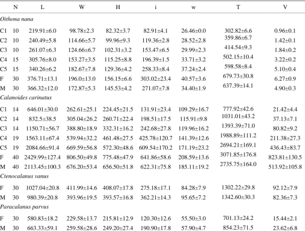
Table 1. Body dimensions (mean ± standard deviation in µm) and estimated biovolume (mean ± standard deviation x 106µm3) of adults and copepodite stages of O. nana, C. carinatus, C. vanus and P. parvus. L, W and H prosome length, width and height, respectively; i and w, urosome length and width, respectively, T total length, V biovolume.
N L W H i w T V
Oithona nana
C1 10 219.91±6.0 98.78±2.3 82.32±3.7 82.91±4.1 26.46±0.0 302.82±6.6 0.96±0.1 C2 10 240.49±5.8 114.66±5.7 99.96±9.3 119.36±2.8 28.52±2.8 359.86±6.7 1.42±0.1 C3 10 261.07±6.3 124.66±6.7 102.31±3.2 153.47±6.5 29.99±2.3 414.54±9.3 1.84±0.2 C4 15 305.76±8.0 153.27±3.5 115.25±8.8 196.39±1.5 33.71±3.2 502.15±10.4 3.22±0.2 C5 15 340.26±6.2 182.67±7.8 129.36±4.2 258.33±8.4 37.24±2.4 598.58±8.4 5.10±0.4 F 30 376.71±13.1 196.0±13.0 156.15±6.6 303.02±23.4 40.57±3.6 679.73±30.8 6.27±0.9 M 30 366.32±12.0 172.87±5.3 145.53±4.2 271.07±7.8 34.40±1.9 637.39±14.1 4.90±0.3 Calanoides carinatus
C1 14 646.01±30.0 262.61±25.1 224.45±21.5 131.91±23.4 109.29±16.7 777.92±42.6 21.42±4.4 C2 14 832.5±38.5 305.04±26.2 260.71±22.4 198.51±17.5 115.91±9.8 1031.01±43.2 37.13±7.1 C3 14 1150.71±56.7 388.80±18.9 332.31±16.2 242.68±27.8 119.96±16.2 1393.39±71.0 80.82±9.2 C4 19 1563.11±67.4 539.94±32.2 461.48±27.5 425.78±120.7 141.39±12.6 1988.89±111.2 211.38±27.3 C5 19 2084.66±91.4 669.59±56.8 572.30±48.6 609.54±170.2 171.19±23.2 2694.21±169.1 436.43±83.7 F 40 2429.99±127.4 806.50±49.8 775.48±47.9 641.86±58.6 208.59±13.6 3071.85±176.8 823.81±130.5 M 40 2113.45±100.3 676.20±53.4 656.50±51.8 622.31±75.8 185.11±19.2 2735.75±164.0 513.92±105.8 Ctenocalanus vanus
F 30 1027.04±20.8 411.99±14.6 408.07±17.8 275.18±17.1 84.28±7.9 1302.22±29.8 92.12±7.9 M 30 980.39±20.8 393.96±19.5 393.57±16.8 362.21±14.3 95.65±7.2 1342.60±30.3 82.36±7.3 Paracalanus parvus
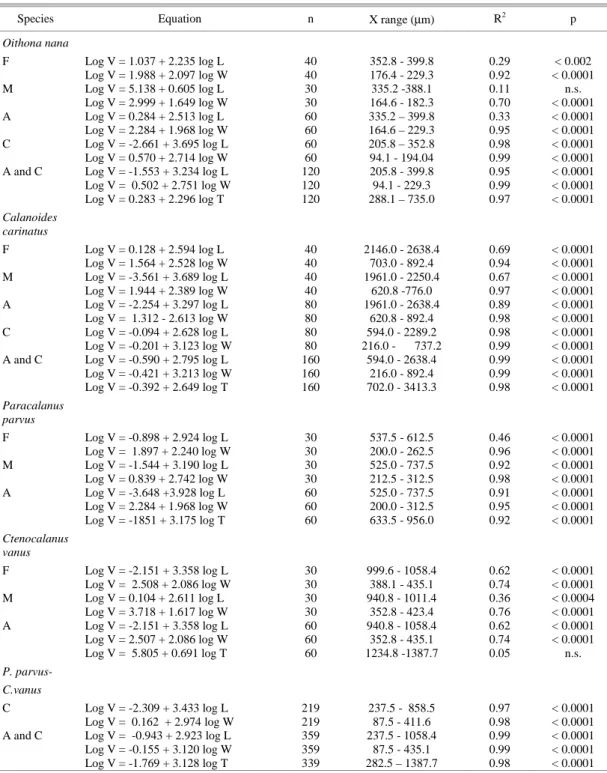
Table 2. Size-biovolume regressions of selected copepod species. V: biovolume (in µm3), L and W: prosome length and width, respectively (in µm), T: total length, F: females, M: males, A: adults and C: copepodites.
Species Equation n X range (µm) R2 p
Oithona nana
F Log V = 1.037 + 2.235 log L 40 352.8 - 399.8 0.29 < 0.002
Log V = 1.988 + 2.097 log W 40 176.4 - 229.3 0.92 < 0.0001
M Log V = 5.138 + 0.605 log L 30 335.2 -388.1 0.11 n.s.
Log V = 2.999 + 1.649 log W 30 164.6 - 182.3 0.70 < 0.0001
A Log V = 0.284 + 2.513 log L 60 335.2 – 399.8 0.33 < 0.0001
Log V = 2.284 + 1.968 log W 60 164.6 – 229.3 0.95 < 0.0001
C Log V = -2.661 + 3.695 log L 60 205.8 – 352.8 0.98 < 0.0001
Log V = 0.570 + 2.714 log W 60 94.1 - 194.04 0.99 < 0.0001
A and C Log V = -1.553 + 3.234 log L 120 205.8 - 399.8 0.95 < 0.0001
Log V = 0.502 + 2.751 log W 120 94.1 - 229.3 0.99 < 0.0001 Log V = 0.283 + 2.296 log T 120 288.1 – 735.0 0.97 < 0.0001 Calanoides
carinatus
F Log V = 0.128 + 2.594 log L 40 2146.0 - 2638.4 0.69 < 0.0001
Log V = 1.564 + 2.528 log W 40 703.0 - 892.4 0.94 < 0.0001
M Log V = -3.561 + 3.689 log L 40 1961.0 - 2250.4 0.67 < 0.0001
Log V = 1.944 + 2.389 log W 40 620.8 -776.0 0.97 < 0.0001
A Log V = -2.254 + 3.297 log L 80 1961.0 - 2638.4 0.89 < 0.0001
Log V = 1.312 - 2.613 log W 80 620.8 - 892.4 0.98 < 0.0001
C Log V = -0.094 + 2.628 log L 80 594.0 - 2289.2 0.98 < 0.0001
Log V = -0.201 + 3.123 log W 80 216.0 - 737.2 0.99 < 0.0001 A and C Log V = -0.590 + 2.795 log L 160 594.0 - 2638.4 0.99 < 0.0001 Log V = -0.421 + 3.213 log W 160 216.0 - 892.4 0.99 < 0.0001 Log V = -0.392 + 2.649 log T 160 702.0 - 3413.3 0.98 < 0.0001 Paracalanus
parvus
F Log V = -0.898 + 2.924 log L 30 537.5 - 612.5 0.46 < 0.0001
Log V = 1.897 + 2.240 log W 30 200.0 - 262.5 0.96 < 0.0001
M Log V = -1.544 + 3.190 log L 30 525.0 - 737.5 0.92 < 0.0001
Log V = 0.839 + 2.742 log W 30 212.5 - 312.5 0.98 < 0.0001
A Log V = -3.648 +3.928 log L 60 525.0 - 737.5 0.91 < 0.0001
Log V = 2.284 + 1.968 log W 60 200.0 - 312.5 0.95 < 0.0001
Log V = -1851 + 3.175 log T 60 633.5 - 956.0 0.92 < 0.0001
Ctenocalanus vanus
F Log V = -2.151 + 3.358 log L 30 999.6 - 1058.4 0.62 < 0.0001
Log V = 2.508 + 2.086 log W 30 388.1 - 435.1 0.74 < 0.0001
M Log V = 0.104 + 2.611 log L 30 940.8 - 1011.4 0.36 < 0.0004
Log V = 3.718 + 1.617 log W 30 352.8 - 423.4 0.76 < 0.0001
A Log V = -2.151 + 3.358 log L 60 940.8 - 1058.4 0.62 < 0.0001
Log V = 2.507 + 2.086 log W 60 352.8 - 435.1 0.74 < 0.0001
Log V = 5.805 + 0.691 log T 60 1234.8 -1387.7 0.05 n.s.
P. parvus-
C.vanus
C Log V = -2.309 + 3.433 log L 219 237.5 - 858.5 0.97 < 0.0001
Log V = 0.162 + 2.974 log W 219 87.5 - 411.6 0.98 < 0.0001 A and C Log V = -0.943 + 2.923 log L 359 237.5 - 1058.4 0.99 < 0.0001 Log V = -0.155 + 3.120 log W 359 87.5 - 435.1 0.99 < 0.0001 Log V = -1.769 + 3.128 log T 339 282.5 – 1387.7 0.98 < 0.0001
The geometric approach has been recently employed by other authors (CALBET et al., 2000; ALCARAZ et al., 2003; GROSJEAN et al., 2004; MC
biovolume from measurements of both the length and width of copepods. Biovolume is then used to make weight estimates. Presumably the geometric method suffers from some of the same drawbacks as the length-weight regression method, but may produce more accurate weights by accounting for changes in width and to some extent the condition factor of the copepod during a stage (KIMMERER et al., 2007).
Prosome width was a better biovolume predictor than prosome length. Similar results were reported by FERNÁNDEZ ARÁOZ (1991) for copepods from Patagonian waters and by PEARRE (1980) on the basis of a large number of species analyzed.
Prosome length is somewhat ambiguous to determine in view of the different morphologies of the main copepod groups and the variety of measuring conventions used by different workers. Besides, width seems to be a more critical dimension than length in prey selection by larval fish (HUNTER, 1981).
A general prosome width-biovolume regression (such as those developed here) including all the developmental stages provided for each species studied, can be potentially useful where detailed identification of stages is not desired (CHISHOLM; ROFF, 1990).
Although a mean biovolume is provided for the adults and copepodite stages of the selected species, it is a known fact that size and, consequently, biovolume of copepods vary both seasonally (VIÑAS; GAUDY, 1996; UYE; SANO, 1998) and geographically (CONOVER; HUNTLEY, 1991) in temperate waters. So, for each study period and area, it is more convenient to estimate the biovolume of targeted species from the size measurements and specific size/biovolume equations. In addition, size is more easily and readily measured than weight (COHEN; LOUGH, 1981).
In the present work, no direct estimates of biovolume were made. However, we validated our biovolume measurements by deriving dry weight from measured copepod body area and comparing it with data from the literature. For that, we chose the equation of HOPCROFT et al. (HOPCROFT et al., 1998) for Oithona nana. Our biovolumes estimated geometrically were converted into dry weight using the above mentioned conversion factors, assuming that ash free dry weight is 73.6 % of dry weight on average (MAUCHLINE, 1998). As a result our indirect estimations of dry weight were, on average, only 4,6% lower than the direct measurements obtained by HOPCROFT et al. (1998).
We have combined the copepodites of P.
parvus and Ctenocalanus in a single equation. This is
a common practical procedure when the species are morphologically very similar and difficult to
distinguish by standard optical analysis in the laboratory (WEBBER; ROFF, 1995).
The importance of investigating the trends in zooplankton biomass in relationship to fish recruitment has been clearly demonstrated (BEAUGRAND et al., 2003; IRIGOIEN et al., 2009). The present findings dealing with important prey of larvae, juveniles and adults of anchovy (Engraulis
anchoita), will contribute to bioenergetic studies
concerning this species.
ACKNOWLEDGEMENTS
We are indebted to Lic. Rubén Negri, head of the “Dinámica del Plancton Marino y Cambio Climático” INIDEP Project for the collection of samples and to Anibal Aubone and Daniel Hernández for statistical advise. We also thank the crew and technicians of the R/V “Capitán Cánepa” for their assistance during the cruises. The comments of the anonymous referees are greatly appreciated. The study was partially supported by grants from the Universidad Nacional de Mar del Plata (UNMDP) Nº 15/E 269 and 15/E 393 to MDV. This is INIDEP Contribution Nº 1584.
REFERENCES
ALCARAZ, M.; SAIZ, E.; CALBET, A.; TREPAT, I.; BROGLIO. E. Estimating zooplankton biomass through image analysis. Mar. Biol., v.143, p. 307-315, 2003. ANGELESCU, V. Ecología trófica de la anchoíta del Mar
Argentino (Engraulidae, Engraulis anchoíta). Parte II. Alimentación, comportamiento y relaciones tróficas en el ecosistema. Serie Contribuciones INIDEP, Mar del Plata, Argentina, v. 409, 83 p., 1982.
BEAUGRAND, G.; BRANDER, K. M.; LINDLEY, J. A.; SOUISSI, S.; REID, P.C. Plankton effect on cod recruitment in the North Sea. Nature, v. 426, p. 661– 664, 2003.
CALBET, A.; LANDRY, M. R.; SCHEINBERG, R. D. Copepod grazing in a subtropical bay: species specific responses to a mid-summer increase in nanoplankton standing stock. Mar. Ecol. Prog. Ser., v. 193, p. 75-84, 2000.
CHISHOLM, L. A.; ROFF, J. C. Size-weight relationships and biomass of tropical neritic copepods off Kingston, Jamaica. Mar. Biol., v. 106, p. 71-77, 1990.
CHOJNACKI, J.; HUSSEIN, M. M. Body length and weight of the dominant copepod species in the Southern Baltic Sea. Zesz. Nauk. Akad. Roln. Szczec, v. 103, p. 53-64, 1983.
CHRISTENSEN, V.; PAULY, D. ECOPATH II-A software for balancing steady-state ecosystem models and calculating network characteristics. Ecol. Model., v. 61, p. 169-185, 1992.
COHEN, R. E.; LOUGH, R. G. Length-weight relationships for several copepods dominant in the Georges Bank-Gulf of Maine area. J. Northw. Atl. Fish. Sci., v. 1, p. 47-52, 1981.
CONOVER, R. J.; HUNTLEY, M. Copepods on ice-covered seas – distribution, adaptations to seasonally limited food, metabolism, growth patterns and life cycle strategies in polar seas. J. Mar. Syst., v. 2, p.1-41,1991. FERNÁNDEZ ARÁOZ, N. C. Individual biomass, based on
body measures of copepod species considered as main forage items for fishes of the Argentine shelf. Oceanologica Acta, v. 14, p. 575-580, 1991.
GROSJEAN, PH.; PICHERAL, M.; WAREMBOURG, C.; GORSKY, G. Enumeration, measurement, and identification of net zooplankton samples using the ZOOSCAN digital imaging system. ICES J. Mar. Sci., v. 61, p. 518-525, 2004.
HOPCROFT, R. R.; ROFF, J. C.; LOMBARD, D. Production of tropical copepods in Kingston Harbour, Jamaica: the importance of small species. Mar. Biol., v. 130, p. 593-604, 1998.
HUNTER, J. R. Feeding ecology and predation of marine fish larvae. In: Marine fish larvae, morphology, ecology and relation to fisheries. Washington: Univ. of Washington Press, 1981.131 p.
IRIGOIEN, X.; FERNÁNDES, J. A.; GROSJEAN, P.; DENIS, K.; ALBAINA, A.; SANTOS, M. Spring zooplankton distribution in the Bay of Biscay from 1998 to 2006 in relation with anchovy recruitment. J. Plankton Res., v. 31, p. 1-17, 2009.
KIMMERER, W. J.; HIRST, A. G.; HOPCROFT, R. R.; MCKINNON, A. D. Estimating juvenile copepod growth rates: corrections, inter-comparisons and recommendations. Mar. Ecol. Prog. Ser., v. 336, p. 187-202, 2007.
MAUCHLINE, J. The biology of calanoid copepods, Advances in Marine Biology, v. 33, Academic Press, New York, 1998. 710 p.
MC KINNON, A. D.; DUGGAN, S.; DE’ATH, G. Mesozooplankton dynamics in inshore waters of the Great Barrier Reef. Estuar. Coast. Shelf. Sci., v. 63, p. 497-511, 2005.
OMORI, M.; IKEDA, T. Methods in Marine Zooplankton Ecology, Wiley- Interscience, New York, 325 pp. 1984.
PÁJARO, M. Alimentación de la anchoíta argentina (Engraulis anchoita Hubbs y Marini, 1935) (Pisces: Clupeiformes) durante la época reproductiva. Rev. Invest. y Des. Pesq., v. 15, p. 111-125, 2002.
PEARRE, S. The copepod width-weight relation and its utility in food chain research. Can. J. Zool., v. 58, p. 1884-1891, 1980.
POSTEL, L., FOCK, H.; HAGEN, W. Biomass and Abundance. In: ICES Zooplankton Methodology Manual, Academic Press, London, 2000, p. 83-192. RAMÍREZ, F. C. Zooplancton y producción secundaria.
Parte I: Variación y distribución estacional de los copépodos. Contr. Inst. Nac. de Invest. y Des. Pesq., v. 383, p. 202-212, 1981.
UYE, S.; SANO, K., Seasonal variations in biomass, growth rate and production rate of the small cyclopoid copepod Oithona davisae in a temperate eutrophic inlet. Mar. Ecol. Prog. Ser., v. 163, p. 37-44, 1998.
VIÑAS, M. D.; GAUDY, R. Annual cycle of Euterpina acutifrons (Copepoda: Harpacticoida) in the Gulf of San Matías (Argentina) and in the Gulf of Marseilles (France). Sci. Mar., v. 60, p. 307-318, 1996.
VIÑAS, M. D.; NEGRI, R. M.; RAMÍREZ, F. C.; HERNÁNDEZ, D. Zooplankton assemblages and hydrography in the spawning area of anchovy (Engraulis anchoita) off Río de la Plata estuary (Argentina, Uruguay). Mar. Freshwat. Res., v. 53, p. 1031-1043, 2002.
VIÑAS, M. D.; RAMÍREZ, F. C. Gut analysis of first-feeding anchovy larvae from Patagonian spawning area in relation to food availability. Arch. Fish. Mar. Res., v. 43, p. 321-256, 1996.
WEBBER, M. K.; ROFF, J. C. Annual biomass and production of the oceanic copepod community off Discovery Bay, Jamaica. Mar. Biol., v. 123, p. 481-495, 1995.