Y.-F. Chen and A. Rezine (Eds.): The 12th INFINITY Workshop. EPTCS 39, 2010, pp. 17–31, doi:10.4204/EPTCS.39.2
c
H. Boucheneb & K. Barkaoui This work is licensed under the Creative Commons Attribution License.
semantics
Hanifa Boucheneb
Laboratoire VeriForm, ´Ecole Polytechnique de Montr´eal, P.O. Box 6079, Station Centre-ville, Montr´eal, Qu´ebec,Canada, H3C 3A7
Kamel Barkaoui
Laboratoire CEDRIC, Conservatoire National des Arts et M´etiers, 292 rue Saint Martin, Paris Cedex 03, France [email protected]
This paper deals with the reachability analysis of{P,A}-Time Petri nets ({P,A}-TPN in short) in the context of strong semantics. It investigates the convexity of the union of state classes reached by different interleavings of the same set of transitions. In [6], the authors have considered the T-TPN model and its Contracted State Class Graph (CSCG) [7] and shown that this union is not necessarily convex. They have however established some sufficient conditions which ensure convexity. This paper shows that for the CSCG of{P,A}-TPN, this union is convex and can be computed without computing intermediate state classes. These results allow to improve the forward reachability anal-ysis by agglomerating, in the same state class, all state classes reached by different interleavings of the same set of transitions (abstraction by convex-union).
1
introduction
Petri nets are established as a suitable formalism for modeling concurrent and dynamic systems. They are used in many fields (computer science, control systems, production systems, etc.). Several extensions to time factor have been defined to take into account different features of the system as well as its time constraints. The time constraints may be expressed in terms of stochastic delays of transitions (stochastic Petri nets), fixed values associated with places or transitions ({P,T}-Timed Petri nets), or intervals labeling places, transitions or arcs ({P,T,A}-Time Petri Nets) [9, 11, 13]. For{P,T,A}-Time Petri Nets, there are two firing semantics: Weak Time Semantics (WTS) and Strong Time Semantics (STS). For both semantics, each enabled transition has an explicit or implicit firing interval derived from time constraints associated with places, transitions or arcs of the net. A transition cannot be fired outside its firing interval, but in WTS, its firing is not forced when the upper bound of its firing interval is reached. Whereas in STS, it must be fired within its firing interval unless it is disabled. The STS is the most widely used semantics. There are also server and single-server semantics. The multiple-server semantics allows to handle, at the same time, several time intervals per place (P-TPN), per arc (A-TPN) or per transition (T-TPN) whereas it is not allowed in the single-server semantics.
In [8], the authors have compared the expressiveness of{P,T,A}-TPN models with strong (X−T PN, X∈ {P,T,A}and weak semantics (X−T PN, X∈ {P,T,A}) (see Figure 1). They have established that1:
• For the single-server semantics, bounded{P,T,A}-TPN and safe{P,T,A}-TPN are equally expres-sive w.r.t. timed-bisimilarity and then w.r.t. timed language acceptance.
1A Petri net is bounded iff the number of tokens in each reachable marking is bounded. It is safe iff the number of tokens in
• T-TPN and P-TPN are incomparable models.
• A-TPN includes all the other models.
• The strong semantics includes the weak one for P-TPN and A-TPN, but not for T-TPN.
Figure 1: Comparison of the expressiveness of{P,T,A}-TPNs given in [8]
The reachability analysis of{P,T,A}-TPN is, in general, based on abstractions preserving properties of interest (markings or linear properties). In general, in the abstractions preserving linear properties, we distinguish three levels of abstraction. In the first level, states reachable by time progression may be either represented or abstracted. In the second level, states reachable by the same sequence of transitions independently of their firing times are agglomerated in the same node. In the third level, the agglomer-ated states are considered modulo some equivalence relation: the firing domain of the state class graph (SCG) [4], the bisimulation relation over the SCG of the contracted state class graph (CSCG) [7], the approximations of the zone based graph (ZBG) [5]). An abstract state is then an equivalence class of this relation. Usually, all states within an abstract state share the same marking and the union of their time domains is convex and defined as a conjunction of atomic constraints2. From the practical point of view, the Difference Bound Matrices (DBMs) are a useful data structure for representing and handling efficiently sets of atomic constraints [1].
The classical forward reachability analysis consists of computing, on-the-fly, all abstract states that are reachable from the initial abstract state. The reachability problem is known to be decidable for bounded{P,T,A}-TPN but the reachability analysis suffers from the state explosion problem. For timed models, this problem is accentuated by the fact that, in the state space abstraction, a node represents, in fact, a finite/infinite set of states (abstract state) and interleavings of concurrent transitions lead, in general, to different abstract states.
To attenuate the state explosion problem, the reachability analysis is usually based on an abstrac-tion by inclusion or by convex-union. During the construcabstrac-tion of an abstracabstrac-tion, each newly computed abstract state is compared with the previously computed ones. In the abstractions by inclusion, two ab-stract states, with the same marking, having domains such that one is included in the other are grouped into one node. In the abstractions by convex-union, two abstract states, with the same marking, having domains such that their union is convex (and then can be represented by a single DBM), are grouped into one node. Convex-union abstractions are more compact than inclusion abstractions [10].
How-2An atomic constraint is of the form x−y≤c, x≤c or−x≤c, where x, y are real valued variables representing clocks or
ever, it is known that DBMs are not closed under union and the convex-union test is a very expen-sive operation relatively to the test of inclusion [10]. The convex-union test of n (with n>1) abstract states α1 = (M,D1),α2 = (M,D2), ...αn = (M,Dn) involves computing the smallest enclosing DBM
α = (M,D)of their union, the difference between D and D1,D2, ...Dn−1, and finally checking that this
difference is included in Dn.
Another interesting reachability analysis approach, proposed in [2] for a CSS-like parallel compo-sition of timed automata, consists of computing abstract states in breadth-first manner and at each level grouping, in one abstract state, all abstract states reached by different interleavings of the same set of concurrent transitions. The authors have shown that this union is convex, and then does not need any test of convexity. To use this approach in the context of{P,T,A}-TPN, we need to show that the union of ab-stract states reached by different interleavings of the same set of transitions is convex. In [6], the authors have shown that for the T-TPN model, this union is not necessarily convex in the SCG and the CSCG. This paper shows that for the P-TPN, this union is not necessarily convex in the SCG but is convex in the CSCG. Finally, it shows that these results are also valid for the A-TPN model.
The next section is devoted to the P-TPN model, its semantics, its SCG, its CSCG, and the proof that the union of abstract states (i.e., state classes) reached by different interleavings of the same set of transitions is not necessarily convex in the SCG but is convex in the CSCG. Moreover, this union can be computed directly without computing beforehand intermediate state classes. Section 3 extends the results shown in Section 2 to the A-TPN model. Section 4 contains concluding remarks.
2
P-Time Petri Nets
In this paper, for reasons of clarity, we consider safe P-Time Petri nets.
2.1 Definition and behavior
A P-Time Petri net is a Petri net augmented with time intervals associated with places. Formally, a P-TPN is a tuple(P,T,Pre,Post,M0,Isp)where:
1. P={p1, ...,pm}and T={t1, ...,tn}are nonempty and finite sets of places and transitions such that
(P∩T= /0),
2. Pre and Post map each transition to its preset and postset (Pre, Post : T −→2P,Pre(ti) =◦ti⊆ P,Post(ti) =ti◦⊆P),
3. M0is the initial marking (M0⊆P),
4. Isp is the static residence interval function (Isp : P→Q+×(Q+∪ {∞})),Q+ is the set of
non-negative rational numbers. Isp(pi)specifies the lower↓Isp(pi)and the upper↑Isp(pi)bounds of
the static residence interval in place pi.
Let M⊆P be a marking and ti a transition of T . Transition ti is enabled for M iff all required
tokens for firing ti are present in M, i.e., Pre(ti)⊆M. The firing of ti from M leads to the marking M′ = (M−Pre(ti))∪Post(ti). The set of transitions enabled for M is denoted En(M), i.e., En(M) = {ti∈T |Pre(ti)⊆M}. A transition tk ∈En(M)is in conflict with tiin M iff Pre(tk)∩Pre(ti)6= /0. The
firing of tiwill disable tk.
The P-TPN state is defined as a triplet s= (M,Dead p,I p), where M⊆P is a marking, Dead p⊆M
is the set of dead tokens in M and I p is the residence interval function(I p : M−Dead p→Q+×(Q+∪ {∞})). The initial state of the P-TPN model is s0= (M0,Dead p0,I p0)where Dead p0= /0, I p0(pi) = Isp(pi), for all pi ∈M0. When a token is created in place pi, its residence interval is set to its static
residence interval Isp(pi). The bounds of this interval decrease synchronously with time, until the token
of pi is consumed or dies. A transition ti can fire iff all its input tokens are available, i.e., the lower
bounds of their residence intervals have reached 0, but must fire, without any additional delay, if the upper bound of, at least, one of its input tokens reaches 0. The firing of a transition takes no time.
We define the P-TPN semantics as follows: Let s= (M,Dead p,I p) and s′= (M′,Dead p′,I p′) be two states of a P-TPN, d∈R+a nonnegative real number and tf ∈T a transition of the net.
- We write s→d s′, also denoted s+d, iff the state s′ is reachable from state s by a time progression of d units, i.e.,∀pi∈M−Dead p, d≤ ↑I p(pi), M′=M, Dead p′=Dead p, and∀pj ∈M′−Dead p′, I p′(pj) = [Max(0,↓I p(pj)−d),↑I p(pj)−d]. The time progression is allowed while we do not overpass
residence intervals of all non dead tokens. No token may die by this time progression.
- We write s→tf s′ iff state s′is immediately reachable from state s by firing transition tf, i.e., Pre(tf)⊆ M−Dead p, ∀pi∈Pre(tf),↓I p(pi) =0, M′= (M−Pre(tf))∪Post(tf), Dead p′ =Dead p, and ∀pi∈ M′−Dead p′, I p′(pi) =Isp(pi),if pi∈Post(tf)and I p′(pi) =I p(pi)otherwise.
- We write sErr→s′ iff state s′ is immediately reachable from state s by firing transition Err. Transition
Err is immediately firable from s if there exists no transition firable from s and there is, at least, a token
in M−Dead p s.t. the upper bound of its interval has reached 0 (token to die) i.e., (∀tk ∈En(M− Dead p),∃pj ∈Pre(tk),↓I p(pj)>0), (∃pi∈M−Dead p,↑I p(pi) =0), M′ =M, Dead p′=Dead p∪ {pj∈M−Dead p|↑I p(pj) =0}, and (∀pi∈M′−Dead p′, I p′(pi) =I p(pi)).
According with the above semantics, states from which transition Err is firable, are timelock states3.
Therefore, transition Err allows to detect timelock states and dead tokens, and also to unblock the time progression.
The P-TPN state space is the timed transition system(S,→,s0), where s0is the initial state of the
P-TPN and S={s|s0
∗
→s}is the set of reachable states of the model,→∗ being the reflexive and transitive closure of the relation→defined above.
A run in the P-TPN state space (S,→,s0), starting from a state s, is a maximal sequence ρ =s1 d1
→ s1+d1
t1
→s2 d2
→..., such that s1=s. By convention, for any state si, relation si 0
→si holds. The
sequence d1t1d2t2...is called the timed trace ofρ. The sequence t1t2....is called the untimed trace ofρ.
Runs of the P-TPN are all runs starting from the initial state s0. Its timed (resp. untimed) traces are timed
(resp. untimed) traces of its initial state.
2.2 The SCG and CSCG of P-TPN
The SCG of P-TPN is defined in a similar way as the SCG of T-TPN, except that time constraints are associated with places, and tokens may die. A SCG state class is defined as a tripletα= (M,Dead p,φp) where M⊆P, Dead p⊆M is the set of dead tokens in M andφpis a conjunction of atomic constraints4
characterizing the union of the residence intervals of its non dead tokens. Each place piof M−Dead p
has a variable denoted piinφprepresenting the residence delay of its token (i.e., the waiting time before
its consummation or its death).
3A state s is a timelock state iff no progression of time is possible and no transition is firable from s. 4An atomic constraint is of the form x−y≤c
From the practical point of view,φpis represented by a Difference Bound Matrix (DBM). The DBM
ofφpis a square matrix D of order|M−Dead p|+1, indexed by variables ofφpand a special variable p0whose value is fixed at 0. Each entry di jrepresents the atomic constraint pi−pj≤di j. Hence, entries di0and d0 jrepresent simple atomic constraints pi≤di0and−pj≤d0 j, respectively. If there is no upper
bound on pi−pj with i6=j, di j is set to∞. Entry diiis set to 0. Though the same nonempty domain may
be represented by different DBMs, they have a unique form called canonical form. The canonical form of a DBM is the representation with tightest bounds on all differences between variables, computed by propagating the effect of each entry through the DBM. It can be computed in O(n3), n being the number of variables in the DBM, using a shortest path algorithm, like Floyd-Warshall’s all-pairs shortest path algorithm [1]. Canonical forms make operations over DBMs much simpler [3].
The initial state class isα0= (M0,Dead p0,φp0)where M0 is the initial marking, Dead p0= /0 and
φp0= V pi∈M0
↓Isp(pi)≤pi≤ ↑Isp(pi).
Successor state classes are computed using the following firing rule [4]: Letα = (M,Dead p,φp)be a state class and tf a transition of T . The state class α has a successor by tf (i.e., succ(α,tf)6= /0) iff Pre(tf)⊆M−Dead p and the following formula is consistent5:
φp∧(
^
pf∈Pre(tf),pi∈M−Dead p
pf−pi≤0).
This firing condition means that tf is enabled in M−Dead p and there is a state s.t. the residence delay
of each input token of tf is less or equal to the residence delays of all non dead tokens in M.
If succ(α,tf)6=/0 then succ(α,tf) = (M′,Dead p′,φp′)is computed as follows:
1. M′= (M−Pre(tf))∪Post(tf);
2. Dead p′=Dead p;
3. Setφp′ to φp∧( V
pf∈Pre(tf),pi∈M−Dead p
pf−pi≤0);
4. Rename, inφp′, pf in tf, for all pf ∈Pre(tf);
5. Add constraints: V
pn∈Post(tf)
↓Isp(pn)≤pn−tf ≤ ↑Isp(pn);
6. Replace each variable pi by pi+tf (this substitution actualizes delays (old pi= new pi+tf));
7. Eliminate by substitution tf.
If tf is firable then its firing consumes its input tokens and creates a token in each of its output places.
Step 2) means that no token may die by firing tf. Step 3) isolates states ofα from which tf is firable.
Note that this firing condition implies that∀pf,p′f ∈Pre(tf),pf =p′f and then the firing delay tf of tf
is equal to pf. Step 4) renames variables associated with tokens consumed by tf in tf. Step 5) adds
constraints of the created tokens. The residence interval of a token created by tf is relative to the firing
date of tf. Step 6) updates the delays of tokens not used by tf. Step 7) eliminates variable tf.
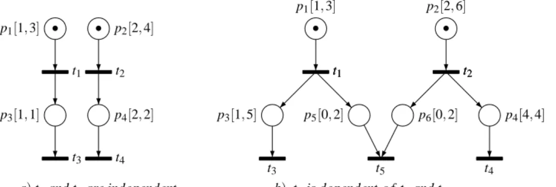
For example, consider the P-TPN shown in Figure 2.a). From its initial SCG state classα0= (p1+
p2,/0,1≤p1≤3 ∧ 2≤p2 ≤4), transition t1 is firable from α0, since 1≤p1≤3 ∧ 2≤ p2≤4∧
p1−p2≤0 is consistent. The firing of t1leads to the state class(p2+p3,/0,0≤p2≤3∧p3=1). Its
formula is derived from the firing condition of t1fromα0as follows: rename p1in t1, add the constraint
t1 t2
t3 t4
p3[1,1]
p1[1,3] p2[2,4]
p4[2,2]
• •
a)t1and t2are independent b) t5is dependent o f t1and t2
p1[1,3] p2[2,6]
p3[1,5] p5[0,2] p6[0,2] p4[4,4]
t1 t2
t1 t2
t3 t5 t4
• •
Figure 2: P-TPNs used to illustrate features of the interleaving in the SCG and the CSCG
1≤p3−t1≤1, replace p2and p3by p2+t1and p3+t1, respectively, and finally eliminate by substitution
t1.
The transition Err is firable fromα= (M,Dead p,φp)iff there is no possibility to reach the intervals
of input places of any enabled transition without overpassing the interval of a non dead token, i.e.,
∃pi∈M−Dead p,s.t.∀tf ∈En(M−Dead p),φp∧( V pf∈Pre(tf)
p
f−pi≤0)is not consistent.
If Err is firable fromα (i.e., succ(α,Err)6= /0), its firing leads to the state class α′ =succ(α,Err) = (M′,Dead p′,φp′) where: M′=M, Dead p′ =Dead p∪ {pi ∈M−Dead p|∀tf ∈En(M−Dead p), φp∧
( V
pf∈Pre(tf)
p
f −pi ≤0) is not consistent }, φ
′
p is obtained from φp by eliminating by substitution all
variables associated with places of Dead p′−Dead p (i.e., by puttingφpin canonical form and eliminating
all variables associated with places of Dead p′−Dead p).
Letα,α′ be two state classes and X∈T∪ {Err}a transition. We writeα −→X α′ iff succ(α,X)6= /0∧α′=succ(α,X). The SCG of the P-TPN is the structure (C,−→,α0) whereα0 is the initial state class andC ={α|α0−→∗ α}is the set of reachable state classes.
Note that dead tokens have no effect on the future behavior. Therefore, we can abstract dead tokens when we compare state classes. Two state classes α = (M,Dead p,φp)and α′= (M′,Dead p′,φp′)are said to be equal iff they have the same set of non dead tokens (i.e., M−Dead p=M′−Dead p′) and the DBMs of their formulas have the same canonical form (i.e.,φp≡φp′).
In the same way as for the SCG of T-TPN [4], we can prove that the SCG of P-TPN is finite and preserves linear properties.
According to the firing rule given above, simple atomic constraints (i.e., atomic constraints of the form pi≤c or−pi ≤c) are not necessary to compute the successor state classes. It follows that all
classes with the same triangular atomic constraints (i.e., atomic constraints of the form p
i−pj≤c) have
the same firing sequences. They can be agglomerated into one node while preserving linear properties of the model. This kind of agglomeration has been successfully used in [7] for the SCG of the T-TPN.
Formally, we define a bisimulation relation, denoted ≃, over the SCG of the P-TPN by: ∀α = (M,Dead p,φp),α′ = (M′,Dead p′,φp′)∈C, let D and D′ be the DBMs in canonical form of φp and
φ′
p, respectively,(M,Dead p,φp)≃(M′,Dead p′,φp′)iff M−Dead p=M′−Dead p′ and ∀pi,pj∈M− Dead p,di j=di j′.
The CSCG of the P-TPN is the quotient graph of the SCG w.r.t. ≃. A CSCG state class is an equivalence class of ≃. It is defined as a triplet β = (M,Dead p,ψp), where ψp is a conjunction of
triangular atomic constraints. The initial CSCG state class isβ0= (M0,Dead p0,ψp0)where M0is the
initial marking, Dead p0=/0 andψp0= V pi,pj∈M0
pi−pj≤ ↑Isp(pi)− ↓Isp(pj).
6), of the firing rule given above, is not needed because the substitution of each piby pi+tf has no effect on triangular atomic constraints ((pi+tf)−(pj+tf) = pi−pj). Steps 6) and 7) are replaced by: Put the resulting formula in canonical form and then eliminate all constraints containing tf.
2.3 Interleaving in the P-TPN state class graph
Note that transition Err, used to detect timelock states and dead tokens, cannot be concurrent to any transition of T . So, there is no interleaving between Err and transitions of T .
Let us first show, by means of a counterexample, that the union of the SCG state classes of a P-TPN, reached by different interleavings of the same set of transitions of T , is not generally convex.
Consider the P-TPN shown in Figure 2.a). From its initial SCG state classα0= (p1+p2,/0,1≤p1≤
3 ∧ 2≤p2≤4), sequences t1t2and t2t1lead respectively to the SCG state classes:
α1= (p3+p4,/0,0≤p3≤1∧p4=2∧ −2≤p3−p4≤ −1)and
α2= (p3+p4,/0,p3=1∧1≤p4≤2∧ −1≤p3−p4≤0).
The union of domains ofα1andα2is obviously not convex.
Consider now the CSCG of the same net. From its initial CSCG state classβ0= (p1+p2,/0,−3≤
p
1−p2≤1), sequences t1t2and t2t1lead to the CSCG state classes:
β1= (p3+p4,/0,−2≤p3−p4≤ −1)andβ2= (p3+p4,/0,−1≤p3−p4≤0), respectively.
The union of domains ofβ1andβ2is convex(−2≤p3−p4≤0).
We will show, in the following, that this result is always valid for the union of all the CSCG state classes reached by different interleavings of the same set of transitions. Let us first establish the firing condition of a sequence of concurrent transitions.
Proposition 1 Letβ = (M,Dead p,ψp)be a CSCG state class, and Tm⊆T a set of transitions enabled and not in conflict in M−Dead p,Ω(Tm)the set of all interleavings of transitions of Tmandω=t1t2...tm∈
Ω(Tm). The successor ofβ byω is non empty (i.e., succ(β,ω)6=/0)6iff the following formula, denoted
ϕp, is consistent:
ψp ∧ t1≤t2≤...≤tm ∧ ^
f∈[1,m]
[ ^
pi∈Pre(tf)
pi=tf ∧ ^
pj∈(M−Dead p)− S l∈[1,f[
Pre(tl)
tf−pj≤0∧
^
k∈[1,f[,pn∈Post(tk)
tf−pkn≤0 ∧ ^
pn∈Post(tf)
↓Isp(pn)≤pnf−tf ≤ ↑Isp(pn) ]
Proof 1 By assumption, all transitions of Tm are not in conflict (i.e., ∀ti,tl ∈Tm s.t. ti 6=tl, Pre(ti)∩ Pre(tl) = /0). The firing condition of the sequence t1t2...tm fromα adds toψp the firing constraints of transitions of the sequence (for f ∈[1,m]). We add for each transition tf of the sequence, a variable, denoted tf, representing its firing delay. The added constraints consist of five blocks. The first block fixes the firing order of transitions of Tm. The second block means that the residence delays of tokens used by each transition tf must be equal to tf. The third and the fourth blocks mean that the firing delay tf is less or equal to the residence delays of tokens that are present (and not dead) when tf is fired (i.e., pj ∈(M−Dead p)− S
l∈[1,f[
Pre(tl)and pn∈ S k∈[1,f[
Post(tk)). The fifth block of constraints specifies the
residence delays of tokens created by tf (i.e., pn∈Post(tf)). Note that pnf denotes the residence delay of the token pncreated by tf.
6succ(β
As an example, consider the P-TPN shown in Figure 2.b) and its initial CSCG state class β0=
(p1+p2,/0,−5≤p1−p2≤1). The firing conditionϕp1of the sequence t1t2is computed as follows:
1) Setϕp1to−5≤p1−p2≤1;
2) Add variables t1and t2and the constraint t1≤t2;
3) Add constraints specifying the firing delays of t1and t2: t1=p1 ∧ t2=p2;
4) Add constraints of tokens created by t1: 1≤p3−t1≤5 ∧ 0≤p5−t1≤2;
5) Add constraints specifying that the firing delay of t2 is less or equal to the residence delays of the
tokens created by t1: t2≤p3 ∧ t2≤p5.
6) Add constraints of tokens created by t2: 4≤p4−t2≤4 ∧ 0≤p6−t2≤2
Then: ϕp1= (−5≤p1−p2≤1) ∧ (t1=p1 ∧t2=p2) ∧ (t1≤t2) ∧
(t2≤p3 ∧ t2≤p5) ∧ (1≤p3−t1≤5 ∧ 0≤p5−t1≤2) ∧ (4≤p4−t2≤4 ∧ 0≤p6−t2≤2)
In the same manner, we obtain the firing conditionϕp2of the sequence t2t1fromβ0:
ϕp2= (−5≤p1−p2≤1) ∧ (t1=p1 ∧ t2=p2) ∧ (t2≤t1) ∧
(t1≤p4 ∧ t1≤p6) ∧ (4≤p4−t2≤4 ∧ 0≤p6−t2≤2) ∧ (1≤p3−t1≤5 ∧ 0≤p5−t1≤2)
Sinceϕp1⇒t1≤p4 ∧t1≤p6andϕp2⇒t2≤p3 ∧ t2≤p5, it follows that:
ϕp1∨ϕp2= (−5≤p1−p2≤1) ∧ (t1=p1 ∧ t2=p2) ∧
(t2≤p
3 ∧ t2≤p5) ∧ (t1≤p4 ∧ t1≤p6) ∧
(4≤p4−t2≤4 ∧ 0≤p6−t2≤2) ∧ (1≤p3−t1≤5 ∧ 0≤p5−t1≤2)
Formula ϕp1∨ϕp2 is the firing condition of t1 and t2 from β0, in any order. Its domain is convex
(representable by a single DBM). The following theorem (Theorem 1) establishes that this result is valid for any set of transitions of T not in conflict and firable from a CSCG state class. The proof of this theorem follows the same ideas as those used in the previous example to show that ϕp1∨ϕp2can be
rewritten as a conjunction of atomic constraints.
Theorem 1 Letβ= (M,Dead p,ψp)be a CSCG state class and Tm⊆T a set of transitions firable from
β and not in conflict inβ.
Then S
ω∈Ω(Tm)
succ(β,ω)6=/0 and S ω∈Ω(Tm)
succ(β,ω) is a state classβ′= (M′,Dead p′,ψ′p)where M′= (M− S
tf∈Tm
Pre(tf)) + S tf∈Tm
Post(tf), Dead p′ =Dead p andψp′ is a conjunction of triangular atomic con-straints that can be computed as follows:
• setψp′ to
ψp ∧ ^
f∈[1,m]
[ ^
pi∈Pre(tf)
p
i=tf ∧ ^
pn∈Post(tf)
↓Isp(pn)≤pnf−tf ≤ ↑Isp(pn) ∧
^
pj∈(M−Dead p)− S l∈[1,m]
Pre(tl)
tf−pj≤0 ∧ ^
k∈[1,m],pn∈Post(tk)
tf−pkn≤0 ]
• Putψp′ in canonical form, then eliminate variables t1,t2, ...,tmand variables associated with their
input places.
Proof 2 If transitions of Tmare all firable fromβ and not in conflict then the firing of one of them cannot disable the others. So, all sequences ofΩ(Tm)are firable fromβ. Then: S
ω∈Ω(Tm)
succ(β,ω)6= /0. Let us
first rewrite the firing conditionϕp, given in Proposition 1, of the sequenceω=t1t2....tm, so as to isolate the part that is independent from the firing order. In other words, let us show that:ϕp≡
ψp ∧ t1≤t2≤...≤tm ∧ ^
f∈[1,m]
[ ^
pi∈Pre(tf)
pi=tf ∧ ^
pn∈Post(tf)
↓Isp(pn)≤pnf−tf ≤ ↑Isp(pn)∧
^
pj∈(M−Dead p)− S l∈[1,m]
Pre(tl)
tf−pj≤0 ∧ ^
k∈[1,m],pn∈Post(tk)
tf−pkn≤0]
Consider the following sub-formula, denotedϕ1, ofϕp:
t1≤t2...≤tm ∧ ^ f∈[1,m]
[ ^
pi∈Pre(tf)
pi=tf ∧ ^
pn∈Post(tf)
↓Isp(pn)≤pnf−tf ≤ ↑Isp(pn)]
This formula implies that: (1) ∀f ∈[1,m],∀l∈[f,m],tf ≤tl.
(2) ∀f∈[1,m],∀l∈[f,m],∀pj∈Pre(tl),tf ≤tl=pj.
Then: (2’)ϕ1⇒ V
f∈[1,m],pj∈ S l∈[f,m]
Pre(tl)
tf −pj≤0.
(3) ∀f∈[1,m],∀l∈[f,m],∀pn∈Post(tl),tf ≤tl≤pln.
Then: (3’)ϕ1⇒ V
f∈[1,m],l∈[f,m],pn∈Post(tl)
tf−pln≤0.
Consider now the following sub-formula, denotedϕ2, ofϕp: ^
f∈[1,m],pj∈(M−Dead p)− S l∈[1,f[
Pre(tl)
tf−pj≤0
From (2’), it follows that constraints (2) are redundant in the partϕ2ofϕp and then can be eliminated from the partϕ2ofϕ, without altering the domain ofϕp:
^
f∈[1,m],pj∈(M−Dead p)− S l∈[1,m[
Pre(tl)
tf−p j≤0
Letϕ3be the following part ofϕ:
^
f∈[1,m],l∈[1,f[,pn∈Post(tl)
tf−pln≤0
From (3’), it follows that constraints (3) are redundant in the partϕ1ofϕpand then can be added to the partϕ3ofϕp, without altering the domain ofϕp:
^
f∈[1,m],l∈[1,m],pn∈Post(tl)
tf−pln≤0
Therefore,ϕp≡
^
f∈[1,m]
[ ^
pi∈Pre(tf)
pi=tf ∧ ^
pn∈Post(tf)
↓Isp(pn)≤pnf−tf ≤ ↑Isp(pn)∧
^
pj∈(M−Dead p)− S l∈[1,m]
Pre(tl)
tf−pj≤0 ∧ ^
k∈[1,m],pn∈Post(tk)
tf−pkn≤0 ]
We have rewritten the firing condition of the sequence t1t2...tm so as to isolate the part t1≤t2...≤tm fixing the firing order from the other part, which is independent of the firing order. It follows that the firing condition of transitions of Tmin any order, denotedφp′, is:
ψp ∧ ^
f∈[1,m]
[ ^
pi∈Pre(tf)
pi=tf ∧ ^
pn∈Post(tf)
↓Isp(pn)≤pnf−tf ≤ ↑Isp(pn)∧
^
pj∈(M−Dead p)− S l∈[1,m]
Pre(tl)
tf−pj≤0 ∧ ^
k∈[1,m],pn∈Post(tk)
tf−pkn≤0 ]
To obtain the formula ofβ′, it suffices to putφp′ in canonical form and then eliminates variables associ-ated with transitions of Tmand their input places.
Theorem 1 is also valid for unsafe P-TPNs in the context of multiple-server semantics. The proof of this claim is similar, except that markings, presets and postsets of transitions are multisets over places. In this case, a variable is associated with each token (instead of each place). Transitions can be multi-enabled. Each enabling instance of a transition is defined as a couple composed by the name of the transition and the multiset of tokens participating in its enabling. Its firing delay depends on time con-straints of its tokens. A variable is associated with each enabling instance of the same transition. In the next section, we will extend the result established in Theorem 1 to the A-TPN model.
3
A-Time Petri Nets
The A-TPN model is the most powerful model in the class of{P,T,A}-TPN [8]. Like in P-TPN, A-TPN uses the notion of availability intervals of tokens but each token of a place p has an availability interval per output arc of p, whereas, in P-TPN, each token has only one availability interval. As for P-TPN, we consider, in the following, safe A-TPN.
Formally, A-TPN is a tuple(P,T,Pre,Post,M0,Isa)where:
1. P, T , Pre, Post and M0are defined as for P-TPN,
2. Let IE={(pi,tj)∈P×T|pi∈Pre(tj)}be the set of input arcs of all transitions. Isa : IE→Q+×
(Q+∪ {∞}) is the static availability interval function. Isa(p
i,tj) specifies the lower↓Isa(pi,tj)
and the upper↑Isa(pi,tj)bounds of the static availability interval of tokens of pi for tj.
Since, in A-TPN, intervals are associated with arcs connecting places to transitions, the notion of dead tokens of the P-TPN model is replaced by dead arcs. If a place pi is marked and connected to a
transition tj, the arc(pi,tj)will die if the residence time of the token of pi overpasses the availability
interval of the arc(pi,tj). To detect dead arcs, we use the special transition Err, as for the P-TPN model.
Let EE(M) ={(pi,tj)∈M×T | pi∈Pre(tj)}be the set of enabled arcs in M. The A-TPN state is
s0= (M0,Deada0,Ia0)where Deada0= /0, Ia0(pi,tj) =Isa(pi,tj), for all (pi,tj)∈EE(M0). When a
token is created in place pi, the availability interval of each output arc(pi,tj)is set to its static interval Isa(pi,tj) and then decreases, synchronously with time, until the token within pi is consumed or the
arc dies. A transition tf can fire iff all its input arcs are not dead and have reached their availability
intervals, i.e., the lower bounds of the intervals of its input arcs have reached 0. But, it must fire, without any additional delay, if the upper bound of, at least, one of its input arcs has reached 0. The firing of a transition takes no time.
The A-TPN state space is the timed transition system(S,→,s0), where s0is the initial state of the
A-TPN and S={s|s0→∗ s}is the set of reachable states of the model,→∗ being the reflexive and transitive
closure of the relation→defined as follows.
Let s= (M,Deada,Ia),s′= (M′,Deada′,Ia′)be two A-TPN states, d∈R+,tf ∈T ,
- s→d s′, iff∀(pi,tj)∈EE(M)−Deada, d≤ ↑Ia(pi,tj), M′=M, Deada′=Deada and ∀(pk,tl)∈ EE(M′)−Deada′,Ia′(p
k,tl) = [Max(↓Ia(pk,tl)−d,0),↑Ia(pk,tl)−d]. The time progression is allowed
while we do not overpass intervals of all non dead arcs of EE(M′).
- s→tf s′ iff state s′ is immediately reachable from state s by firing transition tf, i.e., Pre(tf)× {tf} ⊆ EE(M)−Deada, ∀pi∈Pre(tf),↓Ia(pi,tf) =0, M′= (M−Pre(tf))∪Post(tf), Deada′ =Deada−
(Pre(tf)×T), and∀(pk,tl)∈EE(M′)−Deada′, Ia′(pk,tl) =Isa(pk,tl),if pk∈Post(tf)and Ia′(pk,tl) = Ia(pk,tl) otherwise. It means that all input arcs of tf are enabled, not dead and have reached their
availability intervals. The firing of tf consumes tokens of its input places and produces tokens in its
output places (one token per output place). The consumed tokens and their output arcs are removed. The produced tokens are added to the marking. The availability intervals of their output arcs are set to their static availability intervals.
- sErr→ s′ iff state s′ is immediately reachable from state s by firing transition Err. Transition Err is immediately firable from s if there no transition of T firable from s and there is at least an arc in
EE(M)−Deada s.t. the upper bound of its interval has reached 0 i.e.,(∀tk ∈T s.t. Pre(tk)× {tk} ⊆ EE(M)−Deada,∃pj∈Pre(tk),↓Ia(pj,tk)>0),(∃(pi,tl)∈EE(M)−Deada,↑Ia(pi,tl) =0), M′=M, Deada′ =Deada∪ {(pj,tl)∈EE(M)−Deada|↓Ia(pj,tl)) =0}, and (∀(pi,tj) ∈EE(M′)−Deada′, Ia′(pi,tj) =Ia(pi.tj)).
3.1 The CSCG of the A-TPN
The definition of the CSCG of the P-TPN is extended to the A-TPN by replacing the notion of dead tokens by dead arcs and constraints on availability of tokens by those of arcs. The CSCG state class of A-TPN is defined as a tripletγ= (M,Deada,φa)where M⊆P is a marking, Deada⊆EE(M)is the set
of dead arcs in EE(M)andφais a conjunction of triangular atomic constraints over variables associated
with non dead arcs of EE(M). Each arc(pi,tj)of(EE(M)−Deada)has a variable, denoted pti j inφa,
representing its availability interval.
The initial CSCG state class is:γ0= (M0,Deada0,ψa0)where M0⊆P is the initial marking, Deada0=
/0 andψa0= V
(pi,tj)∈EE(M0),(pk,tl)∈EE(M0)
pti j−pkl≤ ↑Isa(pi,tj)− ↓Isa(pk,tl).
Successor state classes are computed using the following firing rule: Let γ= (M,Deada,ψa)be a
state class and tf a transition of T . The state class γ has a successor by tf (i.e., succ(γ,tf)6= /0) iff Pre(tf)× {tf} ⊆EE(M)−Deada and the following formula is consistent:
ψa∧(
^
pi∈Pre(tf),(pj,tk)∈EE(M)−Deada
This firing condition means that tf is enabled in M, its input arcs are not dead, and there is a state s.t. the
input arcs of tf will reach their intervals before overpassing intervals of all non dead arcs in EE(M).
If succ(γ,tf)6= /0 then succ(γ,tf) = (M′,Deada′,ψa′)is computed as follows:
1. M′= (M−Pre(tf))∪Post(tf);
2. Deada′=Deada−(Pre(tf)×T)
3. Setψa′ to ψa∧( V
pi∈Pre(tf),(pj,tk)∈EE(M)−Deada
pti f ≤ptjk);
4. Replace variables pti f associated with input arcs of tf by tf;
5. Add constraints V
pn∈Post(tf),tl∈p◦n
↓Isa(pn,tl)≤ptnl−tf ≤ ↑Isa(pn,tl);
6. Putψa′ in canonical form and then eliminate tf.
If tf is firable then its firing consumes its input tokens and creates tokens in its output places (one token
per output place). The consumed tokens and their output arcs are eliminated. Step 3) isolates states ofγ from which tf is firable (i.e., states where input arcs of tf reach their availability interval before
overpassing the availability intervals of all non dead enabled arcs). This step implies that for all pi,pj∈ Pre(tf),pti f =ptj f. Step 4) replaces all these equal variables by tf. Steps 5) adds the time constraints
of the created tokens. Step 6) putsψa′ in canonical form before eliminating variable tf.
3.2 Interleaving in the CSCG of A-TPN
The following theorem extends, to A-TPN, the result established in Theorem 1.
Theorem 2 Letγ= (M,Deada,ψa)be a CSCG state class and Tm⊆T a set of transitions firable from
γand not in conflict inγ.
Then S
ω∈Ω(Tm)
succ(γ,ω)6= /0 and S ω∈Ω(Tm)
succ(γ,ω) is a state class γ′ = (M′,Deada′,ψa′) where M′= (M− S
tf∈Tm
Pre(tf))∪ S tf∈Tm
Post(tf), Deada′ =Deada−( S tf∈Tm
Pre(tf)×T) and ψa′ is a conjunction of triangular atomic constraints that can be computed as follows:
• Setψa′ to
ψa ∧ ^
f∈[1,m]
[ ^
pi∈Pre(tf)
pi f =tf ∧ ^
pn∈Post(tf),tl∈p◦n
↓Isa(pn,tl)≤pnlf −tf ≤ ↑Isa(pn,tl) ∧
^
(pj,tk)∈(EE(M)−Deada)− S
l∈[1,m] Pre(tl)×T
tf−pjk≤0 ∧ ^
k∈[1,m],pn∈Post(tk),tl∈p◦n
tf−pknl≤0 ]
• Putψa′ in canonical form, then eliminate variables t1,t2, ...,tmand variables associated with their
input places.
• Rename each variable pnlf ,s.t. pn∈Post(tf),tl ∈p◦nand f ∈[1,m], in pnl.
Proof 3 We first extend the firing condition of a sequence ω =t1t2...tn ofΩ(Tm) given in Proposition 1 to the case of A-TPN.ω is firable fromγ (i.e., succ(β,ω)) iff the following formula, denoted ϕa is consistent:
^
f∈[1,m]
[ ^
pi∈Pre(tf)
pi f =tf ∧ ^
(pj,tk)∈(EE(M)−Deada)− S
l∈[1,f[
(Pre(tl)×T)
tf−pjk≤0∧
^
k∈[1,f[,pn∈Post(tk),tl∈p◦n
tf−pknl≤0 ∧ ^
pn∈Post(tf),tl∈p◦n
↓Isa(pn,tl)≤pnlf −tf ≤ ↑Isa(pn,tl) ]
The firing condition of the sequence t1t2...tmfromγ adds toψafor each transition tf of the sequence, a variable, denoted tf, representing its firing delay and five blocks of constraints. The first block fixes the firing order of transitions of Tm. The second block means that the residence delays of arcs used by each transition tf must be equal to tf. The third and the fourth blocks mean that the firing delay tf is less or equal to the residence delays of all enabled and non dead arcs present when tf is fired (i.e.,(pj,tk)∈
(EE(M)−Deada)−( S
l∈[1,f[
Pre(tl)×T)and(pn,tl)s.t. pn∈ S k∈[1,f[
Post(tk)and tl∈p◦n). The fifth block of
constraints specifies the residence delays of arcs enabled by tf (i.e.,(pn,tl)s.t. pn∈Post(tf)and tl∈p◦n). The rest of the proof follows the same steps as the proof of Theorem 1. In other words, let us show that
ϕa≡ ψa ∧ t1≤t2≤...≤tm ∧ ^
f∈[1,m]
[ ^
pi∈Pre(tf)
pi f =tf ∧ ^
pn∈Post(tf),tl∈p◦n
↓Isa(pn,tl)≤pnlf −tf ≤ ↑Isa(pn,tl)∧
^
(pj,tk)∈(EE(M)−Deada)− S
l∈[1,m] Pre(tl)×T
tf−pjk≤0 ∧ ^
k∈[1,m],pn∈Post(tk),tl∈p◦n
tf−pknl≤0 ]
Consider the following sub-formula, denotedϕ1, ofϕa:
t1≤t2...≤tm ∧ ^ f∈[1,m]
[ ^
pi∈Pre(tf)
pi f =tf ∧ ^
pn∈Post(tf),tl∈p◦n
↓Isa(pn,tl)≤pnlf −tf ≤ ↑Isa(pn,tl)]
This formula implies that: (1) ∀f ∈[1,m],∀k∈[f,m],tf ≤tk. (2) ∀f∈[1,m],∀k∈[f,m],∀pj∈Pre(tk),tf ≤tk=pjk.
Then: (2’)ϕ1⇒ V
f∈[1,m],k∈[f,m],pj∈Pre(tk)
tf−p jk≤0.
(3) ∀f∈[1,m],∀k∈[f,m],∀pn∈Post(tk),∀tl∈p◦n,tf ≤tk≤pknl.
Then: (3’)ϕ1⇒ V
f∈[1,m],k∈[f,m],pn∈Post(tk),tl∈p◦n
tf−pk nl ≤0.
Consider the following sub-formula, denotedϕ2, ofϕa: ^
f∈[1,m],(pj,tk)∈(EE(M)−Deada)− S l∈[1,f[
Pre(tl)×T
tf−pjk≤0
From (2’), it follows that constraints (2) are redundant in the partϕ2ofϕa and then can be eliminated from the partϕ2ofϕa, without altering the domain ofϕa:
^
f∈[1,m],(pj,tk)∈(EE(M)−Deada)− S
l∈[1,m[ Pre(tl)×T
tf−pjk≤0
Letϕ3be the following part ofϕa:
^
f∈[1,m],k∈[1,f[,pn∈Post(tk),tl∈p◦n
From (3’), it follows that constraints (3) are redundant in the partϕ1ofϕaand then can be added to the partϕ3ofϕa, without altering the domain ofϕa:
^
f∈[1,m],k∈[1,m],pn∈Post(tk),tl∈p◦n
tf−pk nl≤0
Therefore,ϕa≡ψa ∧ t1≤t2≤...≤tm ∧ ^
f∈[1,m]
[ ^
pi∈Pre(tf)
pi f =tf ∧ ^
pn∈Post(tf),tk∈p◦n
↓Isa(pn,tk)≤pnkf −tf ≤ ↑Isa(pn,tk)∧
^
(pj,tk)∈(EE(M)−Deada)− S
l∈[1,m] Pre(tl)×T
tf −pjk≤0 ∧ ^
k∈[1,m],pn∈Post(tk),tl∈p◦n
tf−pknl ≤0 ]
The firing condition of transitions of Tm in any order, denoted ψa′, is obtained by eliminating the part fixing the firing order. To obtain the formula of γ′, it suffices to put ψa′ in canonical form and then eliminate variables associated with transitions of Tmand their input places.
The extension of this result to unsafe A-TPN is straightforward by considering multisets of tokens, multisets of enabled arcs, and associating a variable with each instance of multiple enabled arcs. Each enabled transition is defined by the name of the transition and a set of enabled arcs.
Using the translation into A-TPN of the P-TPN shown in Figure 2.a), we prove that the union of the SCG state classes of the A-TPN reached by different interleavings of the same set of transitions is not necessarily convex7. Indeed, its initial SCG state class (p1+p2,/0,1≤ pt11≤3 ∧ 2≤ pt22≤4),
sequences t1t2 and t2t1 lead respectively to the SCG state classes: (p3+p4,/0,0≤ pt33 ≤1∧pt44=
2∧ −2≤pt
33−pt44≤ −1)and(p3+p4,/0,pt33=1∧1≤pt44≤2∧ −1≤pt33−pt44≤0). The union
of their domains is not convex.
4
Conclusion
In this paper, we have considered the P-TPN and A-TPN models, their SCG and CSCG. We have investigated the convexity of the union of state classes reached by different interleavings of the same set of transitions. We have shown that this union is not convex in the SCG but is convex in the CSCG. This result allows to use the reachability analysis approach proposed in [2], which reduces the redundancy caused by the interleaving semantics.
This result is however not valid for the T-TPN [6], in spite of the fact that A-TPN is the most powerful model. This could be explained by the fact that the firing interval of a transition refers to the instant when it becomes enabled in T-TPN, whereas, in{P,A}-TPN, it is equal to the intersection of intervals of all its input tokens/arcs. In T-TPN, the firing interval can be related to the last transition of a sequence and then dependent of the firing order. For example, consider the net shown in Figure 2.b) and suppose that intervals attached to places are moved to be attached to their output transitions. The firing of transitions
t1and t2, in any order, will enable transition t5. But, the firing interval of t5is related to t2in t1t2, whereas
it is related to t1in t2t1. The union of the CSCG state classes reached by t1t2and t2t1from the initial state
class is: (p3+p4+p5+p6,(−8≤t3−t4≤1∧ −6≤t3−t5≤1∧2≤t4−t5≤4)∨(−3≤t3−t4≤
2∧ −1≤t3−t5≤5∧1≤t4−t5≤4)). Its domain is not convex.
7The P-TPN is translated into A-TPN by replacing the static residence interval function Isp by Isa defined by:∀p
i∈P,tj∈
Therefore, A-TPN is more powerful than T-TPN and also more suitable for abstractions by convex-union. However, the translation of T-TPN into A-TPN is not easy and needs to add several places and transitions [8], which may offset the benefits of abstractions by convex-union. The choice of the appropriate{P,T,A}-TPN model for a given problem should be a good compromise between the easiness of modeling the problem and the verification complexity.
As immediate perspective, we will use the results established here and in [6] to investigate the exten-sion, to{P,T,A}-TPN, of the reachability approach proposed in [12] for a variant of safe P-TPN. In this variant, there are two kinds of places (behaviour and constraint places) and each transition can have at most one behaviour place in its preset. A transition is firable, if the age of its behaviour place reaches its static residence interval. It must be fired before overpassing this interval, unless it is disabled.
References
[1] G. Behrmann, P. Bouyer, K. G. Larsen, and R. Pel´anek Lower and upper bounds in zone-based abstractions
of timed automata, International Journal on Software Tools for Technology Transfer Volume 8(3), 2006.
[2] R. Ben Salah, M. Bozga and O. Maler, On Interleaving in Timed Automata, CONCUR’06, 465-476, volume 4137 of LNCS, 2006.
[3] Bengtsson, J.: Clocks, DBMs and States in Timed Systems, PhD thesis, Dept. of Information Technology,
Uppsala University, 2002.
[4] B. Berthomieu and F. Vernadat, State class constructions for branching analysis of Time Petri nets, volume 2619 of LNCS, 2003.
[5] H. Boucheneb, G. Gardey, and O. (H.) Roux. TCTL model checking of time Petri nets, Journal of Logic and Computation, 19(6):1509-1540, December 2009.
[6] H. Boucheneb and K. Barkaoui, Covering steps graphs of time Petri nets In Proc. of the 10th International Workshop on Verification of Infinite-State Systems (INFINITY), 2008.
[7] H. Boucheneb and H. Rakkay, A more efficient time Petri net state space abstraction useful to model checking
timed linear properties In journal of Fundamenta Informaticae, volume 88, number 4, pp 469-495, 2008.
[8] M. Boyer and O. H. Roux,On the compared expressiveness of arc, place and transition time Petri Nets, journal Fundamenta Informaticae, vol. 88, no3, pages 225-249, 2008.
[9] W. Khansa, J.-P Denat and S. Collart-Dutilleul, P-Time Petri Nets for manufacturing systems, International Workshop on Discrete Event Systems, WODES’96, pp 94-102, 1996.
[10] R. Hadjidj and H. Boucheneb, Improving state class constructions for CTL* model checking of Time Petri
Nets, International Journal on Software Tools Technology Transfer (STTT), volume 10, number 2, pp
167-184, 2008.
[11] P. M. Merlin, A study of the recoverability of computing systems., Department of Information and Computer Science, University of California, Irvine CA, 1974.
[12] C. J. Myers, T. G. Rokicki, T. H.-Y. Meng, POSET timing and its application to the timed cirucits, in IEEE Transactions on CAD, 18(6), 1999.
![Figure 1: Comparison of the expressiveness of {P,T,A}-TPNs given in [8]](https://thumb-eu.123doks.com/thumbv2/123dok_br/16482571.199966/2.918.288.631.211.427/figure-comparison-expressiveness-p-t-tpns-given.webp)