www.geosci-model-dev.net/9/4405/2016/ doi:10.5194/gmd-9-4405-2016
© Author(s) 2016. CC Attribution 3.0 License.
Terrestrial ecosystem process model Biome-BGCMuSo v4.0:
summary of improvements and new modeling possibilities
Dóra Hidy1, Zoltán Barcza2, Hrvoje Marjanovi´c3, Maša Zorana Ostrogovi´c Sever3, Laura Dobor2,14,
Györgyi Gelybó4, Nándor Fodor5, Krisztina Pintér1, Galina Churkina6,15, Steven Running7, Peter Thornton8, Gianni Bellocchi9, László Haszpra10,13, Ferenc Horváth11, Andrew Suyker12, and Zoltán Nagy1
1MTA-SZIE Plant Ecology Research Group, Szent István University, Páter K. u.1., 2103 Gödöll˝o, Hungary 2Department of Meteorology, Eötvös Loránd University, Pázmány P. sétány 1/A., 1117 Budapest, Hungary
3Croatian Forest Research Institute, Department for Forest Management and Forestry Economics, Cvjetno naselje 41,
10450 Jastrebarsko, Croatia
4Institute for Soil Sciences and Agricultural Chemistry, Centre for Agricultural Research, Hungarian Academy of Sciences,
Herman O. út 15., 1163 Budapest, Hungary
5Agricultural Institute, Centre for Agricultural Research, Hungarian Academy of Sciences, Brunszvik u. 2.,
2462 Martonvásár, Hungary
6Institute for Advanced Sustainability Studies e.V., Berliner Strasse 130, 14467 Potsdam, Germany
7Numerical Terradynamic Simulation Group, Department of Ecosystem and Conservation Sciences University of Montana,
Missoula, MT 59812, USA
8Climate Change Science Institute/Environmental Sciences Division, Oak Ridge National Laboratory, Oak Ridge,
TN 37831, USA
9UREP, INRA, 63000 Clermont-Ferrand, France
10Hungarian Meteorological Service, P.O. Box 39, 1675 Budapest, Hungary
11Institute of Ecology and Botany, Centre for Ecological Research, Hungarian Academy of Sciences, Alkotmány u. 2-4.,
2163 Vácrátót, Hungary
12School of Natural Resources, University of Nebraska-Lincoln, 806 Hardin Hall, Lincoln, NE 68588, USA
13Geodetic and Geophysical Institute, MTA Research Centre for Astronomy and Earth Sciences, Csatkai Endre utca 6-8, 9400
Sopron, Hungary
14Czech University of Life Sciences, Faculty of Forestry and Wood Sciences, Department of Forest Protection and
Entomology, Kamýcká 129, 165 21 Prague 6, Czech Republic
15Geography Department, Humboldt University of Berlin, Berlin, Germany Correspondence to:Dóra Hidy ([email protected])
Received: 18 April 2016 – Published in Geosci. Model Dev. Discuss.: 13 May 2016 Revised: 7 October 2016 – Accepted: 7 November 2016 – Published: 7 December 2016
Abstract.The process-based biogeochemical model Biome-BGC was enhanced to improve its ability to simulate car-bon, nitrogen, and water cycles of various terrestrial ecosys-tems under contrasting management activities. Biome-BGC version 4.1.1 was used as a base model. Improvements in-cluded addition of new modules such as the multilayer soil module, implementation of processes related to soil mois-ture and nitrogen balance, soil-moismois-ture-related plant senes-cence, and phenological development. Vegetation
Case studies on a managed forest, cropland, and grassland are presented to demonstrate the effect of model develop-ments on the simulation of plant growth as well as on carbon and water balance.
1 Introduction
The development of climate models has led to the construc-tion of Earth system models (ESMs) with varying degrees of complexity where the terrestrial carbon cycle is included as a dynamic sub-model (Ciais et al., 2013). In some of the ESMs, the atmospheric concentration of carbon dioxide (CO2)is no
longer prescribed by the emission scenarios but it is calcu-lated dynamically as a function of anthropogenic CO2 emis-sion and the parallel ocean and land surface carbon uptake. Focusing specifically on land surface, the carbon balance of terrestrial vegetation can be quantified by state-of-the-art bio-geochemical models and are integral parts of the ESMs.
At present, there is no consensus on the future trajectory of the terrestrial carbon sink (Fig. 6.24 in Ciais et al., 2013; see also Friedlingstein et al., 2014). Some ESMs predict satura-tion of the land carbon sink in the near future while others show that the uptake will stay on track with the increasing CO2emission. This means a considerable uncertainty is
re-lated to the climate–carbon cycle feedback (Friedlingstein et al., 2006; Friedlingstein and Prentice, 2010). The wide range of model data related to the land carbon sink means that the current biogeochemical models have inherent uncertainties which must be addressed.
Biogeochemical models need continuous development to include empirically discovered processes and mechanisms, e.g., acclimation processes describing the dynamic responses of plants to the changing environmental conditions (Smith and Dukes, 2012), regulation of stomatal conductance under elevated CO2concentration (Franks et al., 2013), drought
ef-fect on vegetation functioning (van der Molen et al., 2011), soil moisture control on ecosystem functioning (Yi et al., 2010), and other processes. Appropriate description of hu-man intervention is also essential to adequately quantify lat-eral carbon fluxes and net biome production (Chapin et al., 2006). Staying on track with the new measurement-based findings is a challenging task but necessary to improve our ability to simulate the terrestrial carbon cycle more accu-rately.
The process-based biogeochemical model Biome-BGC is the focus of this study. The model was developed by the Numerical Terradynamic Simulation Group (NTSG), at the University of Montana (http://www.ntsg.umt.edu/project/ biome-bgc), and is widely used to simulate carbon (C), ni-trogen (N), and water fluxes of different terrestrial ecosys-tems such as deciduous and evergreen forests, grasslands, and shrublands (Running and Hunt, 1993; Thornton, 1998;
Thornton et al., 2002; Churkina et al., 2009; Hidy et al., 2012).
Biome-BGC is one of the earliest biogeochemical models that include an explicit N cycle module. It is now clear that climate–carbon cycle interactions are affected by N avail-ability and the CO2 fertilization effect can be limited by the amount of N in ecosystems (Friedlingstein and Prentice, 2010; Ciais et al., 2013). Therefore, the explicit simulation of the N cycle is an essential part of these biogeochemical models (Thornton et al., 2007; Thomas et al., 2013).
sim-ulate the climate change impacts on selected forest plots in central Europe.
Di Vittorio et al. (2010) developed Agro-BGC to simulate the functioning of C4 perennial grasses including a new dis-turbance handler and a novel enzyme-driven C4 photosyn-thesis module.
Wang et al. (2005) applied Biome-BGC to simulate crop-land carbon balance in China. Ma et al. (2011) developed ANTHRO-BGC to simulate the biogeochemical cycles of winter crops in Europe, including an option for harvest and considering allocation to yield.
Trusilova and Churkina (2008) applied Biome-BGC to es-timate the carbon cycle of urban vegetated areas.
Lagergren et al. (2006) used Biome-BGC to estimate the carbon balance of the total forested area in Sweden. Mu et al. (2008) used Biome-BGC to estimate the carbon balance of China. In the paper of Jochheim et al. (2009), forest car-bon budget estimates were presented for Germany based on a modified version of Biome-BGC. Barcza et al. (2009, 2011) used Biome-BGC to estimate the carbon balance of Hungary. Eastaugh et al. (2011) used Biome-BGC to estimate the im-pact of climate change on Norway spruce growth in Aus-tria. Biome-BGC was used within the CARBOEUROPE-IP project as well as in several studies exploiting the related European-scale simulation results (e.g., Jung et al., 2007a, b; Vetter et al., 2008; Schulze et al., 2009; ˇTupek et al., 2010; Churkina et al., 2010).
Hunt et al. (1996) used Biome-BGC in a global-scale simulation and compared the simulated net primary produc-tion (NPP) with satellite-based vegetaproduc-tion index. Hunt et al. (1996) also used an atmospheric transport model cou-pled with Biome-BGC to simulate surface fluxes to estimate the distribution of CO2 within the atmosphere. Churkina et al. (1999) used Biome-BGC in a global-scale multimodel in-tercomparison to study the effect of water limitation on NPP. Churkina et al. (2009) used Biome-BGC in a coupled sim-ulation to estimate the global carbon balance for the present and up to 2030. Biome-BGC is used in the Multiscale synthe-sis and Terrestrial Model Intercomparison Project (MsTMIP) (Huntzinger et al., 2013; Schwalm et al., 2010) as part of the North American Carbon Program.
In spite of its popularity and proven applicability, the model development temporarily stopped at version 4.2. One major drawback of the model was its relatively poor perfor-mance in the simulation of the effect of management prac-tices. It is also known that anthropogenic effects have a ma-jor role in the transformation of the land surface in large spa-tial scales (Vitousek et al., 1998). Some structural problems also emerged, like the simplistic soil moisture module (us-ing one soil layer), lack of new structural developments (see, e.g., Smith and Dukes, 2012), problems associated with phe-nology (Hidy et al., 2012), and lack of realistic response of ecosystems to drought (e.g., senescence).
Our aim was to improve the model by targeting significant structural development, and to create a unified,
state-of-the-art version of Biome-BGC that can be potentially used in Earth system models, as well as in situations where manage-ment and water availability play an important role (e.g., in semi-arid regions) in biomass production. The success and widespread application of Biome-BGC can be attributed to the fact that Biome-BGC strikes a great balance between pro-cess fidelity and tractability: it is relatively easy to use and run, even for non-specialists, but still yields interesting in-sights. The success can also be attributed to the open-source nature of the model code. Following this tradition, we keep the developed Biome-BGC open source. In order to support application of the model, a comprehensive user guide was also compiled (Hidy et al., 2015).
In the present work, the scientific basis of the develop-ments is presented in detail, followed by verification studies in different ecosystems (forest, grassland, and cropland) to demonstrate the effect of the developments on the simulated fluxes and pools.
2 Study sites
Model developments were motivated by the need to improve model simulation for grasslands, croplands, and forests. Here, we demonstrate the applicability of the developed model at three sites on three different plant functional types characterized by contrasting management, climate, and site conditions.
2.1 Grassland/pasture
The large pasture near Bugacpuszta (46.69◦N, 19.60◦E; 111 m a.s.l.) is situated in the Hungarian Great Plain, cover-ing an area of 1074 ha. The study site (2 ha) has been used as pasture for the last 150 years according to archive army maps from the 19th century. The soil surface is characterized by an undulating microtopography formed by winds within an ele-vation range of 2 m. The vegetation is highly diverse (species number over 80) dominated byFestuca pseudovinaHack. ex
Wiesb.,Carex stenophyllaWahlbg.,Cynodon dactylon(L.)
Pers., andPoaspp.
The average annual precipitation is 562 mm and the annual mean temperature is 10.4◦C. According to the FAO classi-fication (Driessen et al., 2001) the soil type is chernozem with a rather high organic carbon content (51.5 g kg−1 for the 0–10 cm top soil; Balogh et al., 2011). The soil texture is sandy loamy sand (sand content 78 %, silt content 9 % in the 0–10 cm soil layer). The pasture belongs to the Kiskun-ság National Park and has been under extensive grazing by a Hungarian grey cattle herd in the last 20 years. Stocking density was 0.23–0.58 animal ha−1during the 220-day
graz-ing period between 2004 and 2012.
Carbon dioxide (CO2) and latent heat flux (LHF) have
this study as input and verification data (Nagy et al., 2007, 2011). The EC station has a measurement height of 4 m and is equipped with a CSAT3 (Campbell Scientific) sonic anemometer and a LI-7500 open-path infrared gas analyzer (IRGA; LI-COR Inc., Lincoln, NE, USA). Air temperature, relative humidity, precipitation, global radiation, and soil temperature are also monitored. Soil water content is mea-sured by CS616 (Campbell Scientific, Shepshed, Leicester-shire, UK) probes. Two probes were inserted horizontally at 3 and 30 cm depth and one was inserted vertically averaging the soil water content of the upper 30 cm soil layer. For model evaluation, measured soil water content at 30 cm depth was used.
Data processing includes spike detection and removal fol-lowing Vickers and Mahrt (1997) and linear detrending to calculate fluctuations from the raw data. To avoid errors caused by the flow disturbance effect of the sensor heads, the correction proposed by van der Molen et al. (2004) was ap-plied. The planar fit method (Wilczak et al., 2001) was used to correct for sonic anemometer tilt. Crosswind correction was applied for sensible heat flux calculation after Liu et al. (2001). The Webb–Pearman–Leuning correction (WPL; Webb et al., 1980) was used to consider the effect of fluctu-ations in air density on the fluxes. Frequency response cor-rections were applied after Moore (1986) to account for the damping effect of sensor line averaging, lateral separation between the IRGA and the sonic anemometer, and the lim-ited time response of the sensors. The gap-filling and flux partitioning methods are based on the nonlinear function be-tween photosynthetically active photon flux density (PPFD) and daytime CO2fluxes, and temperature and nighttime CO2 fluxes (Reichstein et al., 2005).
2.2 C4 cropland
Three production-scale cropland measurement sites were es-tablished in 2001 at the University of Nebraska Agricultural Research and Development Center near Mead, Nebraska, USA, which are the part of the AmeriFlux (http://ameriflux. ornl.gov/) and the FLUXNET global network (http://fluxnet. ornl.gov/). Mead1 (41.17◦N, 96.48◦W; 361 m a.s.l.; 48.7 ha) and Mead2 (41.16◦N, 96.47◦W; 362 m a.s.l.; 52.4 ha) are both equipped with center pivot irrigation systems. Mead3 (41.18◦N, 96.44◦W; 362 m a.s.l.; 65.4 ha) relies on rainfall. Maize is planted each year at Mead1, while Mead2 and Mead3 are in a maize–soybean rotation.
On the Mead sites, the annual average temperature is 10.1◦C and the mean annual precipitation total is 790 mm. Soil at the site is deep silty clay loam consisting of four soil series: Yutan (fine–silty, mixed, superactive, mesic Mol-lic Hapludalfs), Tomek (fine, smectitic, mesic Pachic Argial-bolls), Filbert (fine, smectitic, mesic Vertic ArgialArgial-bolls), and Fillmore (fine, smectitic, mesic Vertic Argialbolls).
The CO2and energy fluxes are measured by an EC system
using an omnidirectional three-dimensional sonic
anemome-ter (model R3, Gill Instruments Ltd., Lymington, UK), an open-path infrared CO2/H2O gas analyzer (model
LI-7500: LI-COR Inc., Lincoln, NE, USA), and a closed-path CO2/H2O system (model LI-6262: LI-COR Inc., Lincoln,
NE, USA). The sensors were mounted 3 m above the ground when the canopy was shorter than 1 m, and later moved to a height of 6 m until harvest when maize was planted (Suyker et al., 2004; Verma et al., 2005).
Raw EC data processing included correction of fluxes for inadequate sensor frequency response (i.e., tube attenuation, sensor separation; Massman, 1991; Moore, 1986). Fluxes were adjusted for flow distortion (Nakai et al., 2006) and the variation in air density due to the transfer of water va-por (Webb et al., 1980; Suyker et al., 2003).
Air temperature and humidity were measured at 3.0 and 6.0 m height (Humitter50Y, Vaisala, Helsinki, Finland). PPFD (LI 190SA Quantum Sensor, LI-COR Inc., Lincoln, NE, USA), net radiation at 5.5 m height (Q*7.1, Radiation and Energy Balance Systems Inc., Seattle, WA, USA), and soil heat flux (0.06 m depth; Radiation and Energy Balance Systems Inc.) were also measured (Verma et al., 2005). Soil water content measured at 0.1 m depth was used in this study (ML2 Thetaprobe, Delta T Devices Ltd, Cambridge, UK).
Green leaf area index (LAI) was determined from destruc-tive sampling. A LI-COR 3100 (LI-COR Inc., Lincoln, NE, USA) leaf area meter was used to measure sampled leaves. Each sampling was from six 1 m row samples from six parts of the field. Aboveground biomass was determined using destructive plant sampling. Plants were cut off at ground level, brace roots were removed, and plants were placed in fine mesh bags. Plants were dried to constant weight. Sub-sequently, the mass of green leaves, stems, reproductive or-gans, and senesced tissue was determined on a per-plant ba-sis. Measured plant populations were used to convert from per-plant basis to a unit-ground-area basis.
The Mead1 site was under no-till management prior to the harvest of 2005. Currently, there is a fall conservation tillage for which approximately one-third of the crop residue is left on the surface. From 2010 to 2013, for a biomass removal study, management at Mead2 was identical to Mead1 (con-tinuous maize, fall conservation tillage, etc.). Management settings of the simulations were based on site records. In this study, the Mead1 site is used for model evaluation.
2.3 Deciduous broad-leaved forest
The Jastrebarsko site (45.62◦N, 15.69◦E; 115 m a.s.l.) is a forest study site situated in a lowland oak forest that is part of the state-owned Pokupsko basin forest complex, located approximately 35 km southwest of Zagreb (Croatia). The for-est compartment where the EC tower for CO2flux measure-ment is located was a 37-year-old mixed stand dominated by
Quercus roburL. (58 %) accompanied by other tree species,
(1 %). Corylus avellana L. andCrataegus monogyna Jacq.
are common in the understory. Oak forests in this area are managed in 140-year rotations. Stands are thinned once ev-ery 10 years ending with regeneration cuts during the last 10 years of the rotation (two or three), aimed at facilitating natural regeneration of the stand and continuous cover of the soil.
Annual mean temperature was 10.6◦C and average an-nual precipitation was 962 mm during the period of 1981– 2010 (data from the National Meteorological and Hydro-logical Service for the Jastrebarsko meteoroHydro-logical station). The average annual depth to the groundwater ranges from 60 to 200 cm (Mayer, 1996). Groundwater level in a 4 m deep piezometer was measured weekly during the vegetation sea-son from 2008 onwards. The forest is partly flooded with stagnating water during winter and early spring due to the heavy soil present at the site. Soil is generally Gleysol with low water conductivity (Mayer, 1996), and according to the World Reference Base for Soil Resources (WRB, 2006), it is classified as Luvic Stagnosol. The soil texture is dominantly clay with 18 % of sand and 28 % of silt fraction in the 0– 30 cm top soil layer (Mayer, 1996).
Carbon dioxide and latent heat flux have been measured by the EC technique since September 2007 (Marjanovi´c et al., 2011a, b). The measurement height at the time of installation was 23 m above ground (3–5 m above the top of the canopy). Since the forest stand grew, the measurement height was el-evated to 27 m in April 2011. The EC system was made up of a sonic anemometer (81 000 V, R.M. Young, USA) and an open-path IRGA (LI-7500, LI-COR Inc., Lincoln, NE) with a sampling rate of 20 Hz. Meteorological measurements cluded soil temperature, incoming shortwave radiation, in-coming and outgoing PPFD, net radiation, air temperature and humidity, soil heat flux, and total rainfall. Soil water con-tent was measured at 0–30 cm depth using two time-domain reflectometers (Marjanovi´c et al., 2011a).
Raw data processing of EC data was made using EdiRe Data Software (University of Edinburgh, United Kingdom) according to the methodology based on the EuroFlux proto-col (Aubinet et al., 2000) with a further adjustment such as the WPL correction (Webb et al., 1980). Quality control was performed after Foken and Vichura (1996). Net ecosystem exchange (NEE) was obtained after taking into account the storage term which was calculated using a profile system de-signed to make sequential CO2concentration measurements (IRGA, SBA-4, PP Systems) from six heights in a 6 min cy-cle. Quality assessment and quality control was made accord-ing to Foken and Vichura (1996). Gap-fillaccord-ing of missaccord-ing data and NEE flux partitioning to gross primary production (GPP) and total ecosystem respiration (TER) was made using online EC data gap-filling and flux partitioning tools (http://www. bgc-jena.mpg.de/~MDIwork/eddyproc/) using the method of Reichstein et al. (2005).
Jastrebarsko forest stand characteristics data include diam-eter at breast height (dbh) and volume distribution by tree
species, weekly tree stem and annual height increment, tree mortality, phenology data, annual litterfall, litterfall C and N content, fine root biomass, net annual root-derived car-bon input, soil texture, and carcar-bon content (Marjanovi´c et al., 2011b; Ostrogovi´c, 2013; Alberti et al., 2014). Data were used either as input in modeling (e.g., groundwater level), for assessing some of the model parameters (e.g., phenol-ogy data) or model evaluation (e.g., EC fluxes, tree increment measurements).
3 Description of base model: Biome-BGC 4.1.1 MPI Our model developments started before Biome-BGC 4.2 was published. The starting point was Biome-BGC v4.1.1 with modifications described in Trusilova et al. (2009). We re-fer to this model as Biome-BGC v4.1.1 MPI version (MPI refers to the Max Planck Institute in Jena, Germany) or orig-inal Biome-BGC. Biome-BGC v4.1.1 MPI version was de-veloped from the Biome-BGC family of models (Thornton, 2000). Biome-BGC is the extension and generalization of the Forest-BGC model to describe different vegetation types in-cluding C3 and C4 grasslands (Running and Coughlan, 1988; Running and Gower, 1991; Running and Hunt, 1993; Thorn-ton, 2000; White et al., 2000; Trusilova et al., 2009).
Biome-BGC uses a daily time step. The model is driven by daily values of minimum and maximum temperatures, pre-cipitation, daytime mean global radiation, and daylight aver-age vapor pressure deficit (VPD). In addition, Biome-BGC uses site-specific data (e.g., soil texture, site elevation, lat-itude), and ecophysiological data (e.g., maximum stomatal conductance, specific leaf area, C : N mass ratios in different plant compartments, allocation of related parameters) to sim-ulate the biogeochemical processes of the given biome. The main simulated processes are photosynthesis, evapotranspi-ration, allocation, litterfall, and C, N, and water dynamics in the litter and soil (Thornton, 2000).
In Biome-BGC, the main parts of the simulated ecosystem are defined as plant, soil and litter. As Biome-BGC explicitly simulates the water, carbon and N balance of the soil–plant system, the most important pools include leaf (C, N, and wa-ter), fine root (C, N), soil (C, N, and wawa-ter), and litter (C, N). C and N pools have additional sub-pools (i.e., so-called actual pools, storage pools, and transfer pools). The actual sub-pools are defined to store the amount of C and N that is available for growth on a given day. The storage sub-pools contain the amount of C and N that will appear during the next year’s growing season (in this sense they are the virtu-alization of seeds or buds). The transfer sub-pools inherit the entire content of the storage pools at the end of a given year. The model simulation has two phases. The first is the spinup simulation (or, in other words, the self-initialization or equilibrium run), which starts with a very low initial level of soil C and N and runs until a steady state is reached under the given climate in order to estimate the initial values of the state variables (Thornton, 2000; Thornton and Rosenbloom, 2005). In the second phase, the normal simulation uses the results of the spinup simulation as initial values for the C and N pools. This simulation is performed for a given predeter-mined time period.
4 Methodological results: model adjustments
Some improvements focusing primarily on the development of the model to simulate carbon and water balance of man-aged herbaceous ecosystems have already been published (Hidy et al., 2012). Previous model developments included structural improvements on soil hydrology and plant phenol-ogy. Additionally, management modules were implemented in order to provide more realistic fluxes for managed grass-lands. We refer to this model version as the modified Biome-BGC (this is the predecessor of the current model).
Several developments have been made since the publica-tion of the Hidy et al. (2012) study. The developments were motivated by multiple factors. Poor agreement of the mod-ified Biome-BGC with available eddy covariance measure-ments made in Hungary over two grassland sites (see Hidy et al., 2012) clearly revealed the need for more sophisticated representation of soil hydrology, especially at the drought-prone, sandy Bugac site. Implementation and benchmarking of the multilayer soil module resulted in several additional developments related, e.g., to the N balance, soil tempera-ture, root profile, soil water deficit effect on plant function-ing, and decomposition of soil organic matter. Lack of man-agement descriptors within the original Biome-BGC moti-vated the development of a broad array of possible manage-ment techniques covering typical grassland, cropland, and forest management practices. Modeling exercises within in-ternational projects revealed additional problems that needed a solution related, e.g., to stomatal conductance (Sándor et al., 2016). Recently published findings (e.g., simulation of
temperature acclimation of respiration; Smith and Dukes, 2012) also motivated our work on model development. Ad-dressing the known issues with the Biome-BGC model re-quired diverse directions, but this was necessary due to the complex nature of the biogeochemical cycles of the soil– plant system. Our overarching aim was to provide a state-of-the-art biogeochemical model that is in the same league as currently available models, such as LPJmL, ORCHIDEE, CLM, JULES, CASA, and others.
The model that we present in this study is referred to as Biome-BGCMuSo (abbreviated as BBGCMuSo, where MuSo refers to a multilayer soil module). Currently, BBGC-MuSo has several versions but hereafter only the latest ver-sion (4.0) is discussed.
In this paper, we provide detailed documentation of all changes made in the model logic compared to the origi-nal model (Biome-BGC v4.1.1). Here, we briefly mention the previously published developments and we provide de-tailed descriptions concerning the new features. In order to illustrate the effect and the importance of the developments, model evaluations are presented for three contrasting sites equipped with EC measurement systems in Sect. 5.
Due to the modifications of the model structure and the implementation of the new management modules, it was nec-essary to modify the structure of the input and output files of the model. Technical details are discussed in the user guide of BBGCMuSo v4.0 (Hidy et al., 2015; http://nimbus.elte. hu/bbgc/files/Manual_BBGC_MuSo_v4.0.pdf).
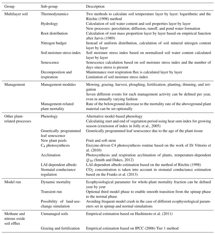
We summarized the model adjustments in Table 1. Within the table, the implemented processes are grouped for clarity. Below, we document the adjustments in detail.
4.1 Multilayer soil
Table 1.Summary of model adjustments. Group refers to major processes represented by collection of modules in Biome-BGCMuSo, while sub-group refers to specific features.
Group Sub-group Description
Multilayer soil Thermodynamics Two methods to calculate soil temperature layer by layer: logarithmic and the Ritchie (1998) method
Hydrology Calculation of soil water content and soil properties layer by layer New processes: percolation, diffusion, runoff, and pond water formation Root distribution Calculation of root mass proportion layer by layer based on empirical function
after Jarvis (1989)
Nitrogen budget Instead of uniform distribution, calculation of soil mineral nitrogen content layer by layer
Soil moisture stress index Soil moisture stress index based on normalized soil water content calculated layer by layer
Senescence Senescence calculation based on soil moisture stress index and the number of days since stress is present
Decomposition and respiration
Maintenance root respiration flux is calculated layer by layer Limitation of soil moisture stress index
Management Management modules Mowing, grazing, harvest, ploughing, fertilization, planting, thinning, and irri-gation
Seven different events for each management activity can be defined per year, even in annually varying fashion
Management-related plant mortality
Rate of the belowground decrease to the mortality rate of the aboveground plant material can be set optionally
Other plant-related processes
Phenology Alternative model-based phenology
Calculating start and end of vegetation period using heat sum index for growing season (extension of index in Jolly et al., 2005)
Genetically programmed leaf senescence
Genetically programmed leaf senescence due to the age of the plant tissue
New plant pools Fruit and soft stem
C4photosynthesis Enzyme-driven C4 photosynthesis routine based on the work of Di Vittorio et al. (2010)
Acclimation Photosynthesis and respiration acclimation of plants, temperature-dependent Q10(Smith and Dukes, 2012)
LAI-dependent albedo LAI-dependent albedo estimation based on the method of Ritchie (1998) Stomatal conductance
regulation
CO2 concentration is taken into account in stomatal conductance estimation based on the Franks et al. (2013)
Model run Dynamic mortality Ecophysiological parameter for whole-plant mortality fraction can be defined year by year
Transient run Optional third model phase to enable smooth transition from the spinup phase to the normal phase
Possibility of land-use-change simulation
Avoiding frequent model crash in the case of different ecophysiological param-eters set in spinup and normal simulations
Methane and nitrous oxide soil efflux
Unmanaged soils Empirical estimation based on Hashimoto et al. (2011)
Grazing and fertilization Empirical estimation based on IPCC (2006) Tier 1 method
accuracy and computational cost. In accordance with the soil layers, we also defined new fluxes within the model. Note that in the Hidy et al. (2012) publication the devel-oped Biome-BGC had only four soil layers, so the seven-layer module is an improvement.
of the given layer. Below 5 m, the soil temperature can be as-sumed equal to the annual average air temperature of the site (Florides and Kalogirou, 2016). Furthermore, in the bottom layer we assume that soil water content (SWC) is equal to the field capacity (constant value) and soil mineral content has a small, constant value (1 kg N ha−1 within the 7 m deep soil
column). The percolated water (and soluble N) to the bottom hydrologically inactive layer is a net loss, while the water (and soluble N) diffused upward from the bottom layer is a net gain for the simulated soil system.
Soil texture and soil bulk density can be defined by the user, layer by layer. If the maximum rooting zone (defined by the user) is greater than 3 m, the roots reach the con-stant boundary soil layer and water uptake can occur from that layer, as well. In previous BBGCMuSo model versions, the soil texture was constant with depth, and the maximum possible rooting depth was 5 m.
4.1.1 Soil thermodynamics
Since some of the soil processes depend on the actual soil temperature (e.g., decomposition of soil organic matter), it is necessary to calculate soil temperature for each active layer. Given the importance of soil temperature (e.g., Sándor et al., 2016), the soil module was also reconsidered in BBGC-MuSo. The daily soil surface temperature is determined after Zheng et al. (1993). The basic equations are detailed in Hidy et al. (2012). An important modification in BBGCMuSo is that the average temperature of the top soil layer (with a thickness of 10 cm) is not equal to the above-mentioned daily surface temperature. Instead, temperature of the active layers is estimated based on an empirical equation with daily time steps.
Two optional empirical estimation methods are imple-mented in BBGCMuSo. The first is a simple method, assum-ing a logarithmic temperature gradient between the surface and the constant temperature boundary layer. This is an im-provement compared to the modified Biome-BGC where a linear gradient was assumed. The second method is based on the soil temperature estimation method of the DSSAT model family (Ritchie, 1998) and the 4M model (Sándor and Fodor, 2012).
4.1.2 Soil hydrology
The C and the hydrological cycles of the ecosystems are strongly coupled due to interactions between soil moisture and stomatal conductance, soil organic matter decomposi-tion, N mineralizadecomposi-tion, and other processes. Accurate esti-mation of the soil water balance is thus essential.
Among soil hydrological processes, the original Biome-BGC only takes into account plant uptake, canopy intercep-tion, snowmelt, outflow (drainage), and bare soil evaporation. We have added the simulation of runoff, diffusion, perco-lation, and pond water formation and enhanced the
simula-tion of the transpirasimula-tion processes in order to improve the soil water balance simulation. Optional handling of season-ally changing groundwater depth (i.e., possible flooding due to elevated water table) is also implemented. In the Hidy et al. (2012) study, only runoff, diffusion, and percolation were implemented (the simulation of these processes has been fur-ther developed since then). Pond water formation and simu-lation of groundwater movement are new features in BBGC-MuSo 4.0.
Estimation of characteristic soil water content values There are four significant characteristic points of the soil wa-ter retention curve: saturation, field capacity, permanent wilt-ing point, and hygroscopic water. Beside volumetric SWC, soil moisture status can also be described by soil water po-tential (PSI; MPa). The Clapp–Hornberger parameter (B;
di-mensionless) and the bulk density (BD; g cm−3), are also
important in soil hydrological calculations (Clapp and Horn-berger, 1978). Soil texture information (fraction of sand and silt within the soil; clay fraction is calculated by the model internally as a residual) for each soil layer are input data for BBGCMuSo. Based on soil texture, other soil properties (characteristic points of SWC,B, BD) can be estimated
inter-nally by the model using pedotransfer functions (Fodor and Rajkai, 2011). The default values are listed in Table 2, which can be adjusted by the user within their plausible ranges.
As in the original Biome-BGC, the PSI at saturation is the function of soil texture in BBGCMuSo:
PSIsat= − {exp [(1.54−0.0095·SAND+0.0063·SILT)
·ln(10)]·9.8·10−5o, (1)
where SAND and SILT are the sand and silt percent fractions of the soil, respectively. In BBGCMuSo, PSI for unsaturated soils is calculated from SWC using the saturation value of SWC (SWCsat) and theBparameter:
PSI=exp
SWC sat
SWC ·ln(B)
·PSIsat. (2)
Pond water and hygroscopic water
In the case of intensive rainfall events, when not all of the precipitation can infiltrate, pond water is formulated at the surface. Water from the pond can infiltrate the soil after the water content of the top soil layer decreases below satura-tion. Evaporation of the pond water is assumed to be equal to potential soil evaporation.
Table 2.Default values of parameters in BBGCMuSo for different soil types. Soil types are identified based on the user-defined sand, silt, and clay fraction of the soil layers based on the soil triangle method.
Sand Loamy Sandy Sandy Sandy Loam Silt Silt Silty Clay Silty Clay
sand loam clay clay loam loam clay loam loam clay
B 3.45 10.45 9.22 5.26 4.02 50 7.71 7.63 6.12 5.39 4.11 12.46
SWCsat 0.4 0.52 0.515 0.44 0.49 0.51 0.505 0.5 0.46 0.48 0.42 0.525
SWCfc 0.155 0.445 0.435 0.25 0.38 0.42 0.405 0.39 0.31 0.36 0.19 0.46
SWCwp 0.03 0.275 0.26 0.09 0.19 0.24 0.22 0.205 0.13 0.17 0.05 0.29
BD 1.60 1.4 1.42 1.56 1.5 1.44 1.46 1.48 1.54 1.52 1.58 1.38
RCN 50 70 68 54 56 64 66 62 58 60 52 72
B(dimensionless): Clapp–Hornberger parameter; SWCsat, SWCfc, SWCwp(m3m−3): SWCs at saturation, at the field capacity and at the wilting point, respectively; BD (g cm−3): bulk density; RCN (dimensionless): runoff curve number.
pool of the top layer can be depleted (approaching hygro-scopic water content). In this case, evaporation and transpi-ration fluxes are limited in BBGCMuSo. Hygroscopic water content is also the lower limit in decomposition calculations (see below).
Runoff
Our runoff simulation method is semi-empirical and uses the precipitation amount and the Soil Conservation Service (SCS) runoff curve number (Williams, 1991). If the precipi-tation is greater than a critical amount which depends on the water content of the topsoil, a fixed part of the precipitation is lost due to runoff and the rest infiltrates the soil. The runoff curve number can be set by the user or can be estimated by the model (Table 2).
Percolation and diffusion
In BBGCMuSo, two calculation methods of vertical soil wa-ter movement are implemented. The first method is based on Richards’ equation (Chen and Dudhia, 2001; Balsamo et al., 2009). A detailed description and equations for this method can be found in Hidy et al. (2012). The second method is the so-called “tipping bucket method” (Ritchie, 1998) which is based on semi-empirical estimation of percolation and diffu-sion fluxes and has a long tradition in crop modeling.
In the case of the first method, hydraulic conductivity and hydraulic diffusivity are used in diffusion and percola-tion calculapercola-tions. These variables change rapidly and signifi-cantly upon changes in SWC. As we already mentioned, for the calculation of the main processes, a daily time step is used. For the calculation of the soil hydrological processes, finer temporal resolution was implemented in the case of the first calculation method (in the case of the tipping bucket method, a daily time step is used).
In BBGCMuSo, the time step (TS; seconds) of the soil water module integration is dynamically changed. In contrast to the modified Biome-BGC (Hidy et al., 2012), the TS is based on the theoretical maximum of soil water flux instead of the amount of precipitation.
As a first step, we calculate water flux data for a short, 1 s TS for all soil layers based on their actual SWC. The most important problem here is the selection of the optimal TS: TS values that are too small result in a slow model run, while TS values that are too large will lead to overestimation of water fluxes. The TS is estimated based on the magnitude of the maximal soil moisture content change in 1 s (1SWCmax;
m3m−3s−1). Equations (3)–(4) describes the calculation of
TS:
TS=10EXPON, (3)
where
EXPON=abs [LV+(DL+3)] if DL+LV<0
EXPON=0 if DL+LV≥0 . (4)
LV is the rounded local value of the maximal soil moisture content change, and DL is the discretization level, which can be 0, 1, or 2 (low, medium, or high discretization level which can be set by the user).
Therefore, if the magnitude of 1SWCmax is
10−3m3m−3s−1 (e.g., SWC increases from 0.400 to 0.401 m3m−3in 1 s), then LV is−3, so TS is 100=1 s (if DL=0). The 1 s TS is necessary if 1SWCmax is above
10−1m3m−3s−1. Using daily TS proved to be adequate
when1SWCmaxwas below 10−8m3m−3s−1.
After calculating the first TS (TSstep1=1 s), water fluxes
are determined by using the precalculated time steps, and the SWC of the layers are updated accordingly. In the next n
steps the calculations are repeated until reaching a threshold (86 400, the number of the seconds in a day). This method helps to avoid the overestimation of the water fluxes while also decreasing the computation time of the model.
4.1.3 Groundwater
supply external information about the depth of the water ta-ble. Groundwater depth is controlled by prescribing the depth of saturated zone (groundwater) within the soil. We note that the groundwater implementations by Pietsch et al. (2003) and by Bond-Lamberty et al. (2007a) are different from our ap-proach as they calculate water table depth internally with the modified Biome-BGC. During the spinup phase of the sim-ulation, the model can only use daily average data for one typical simulation year (i.e., multiannual mean water table depth). During the normal phase, the model can read daily groundwater information defined externally.
The handling of the externally supplied, near-surface groundwater information is done as follows. If the upward-moving water table reaches the bottom border of a simulated soil layer, part of the given layer becomes “quasi-saturated” (99 % of the saturation value), and thus the average soil mois-ture content of the given layer increases. If the water table reaches the upper border of the given soil layer, then the given layer becomes quasi-saturated. The quasi-saturation state allows for the downward flow of water through a sat-uration soil layer, particularly through the last layer. This ap-proach was necessary because of the discrete size of soil lay-ers and the fact that the input groundwater level data consti-tute a net groundwater level. Namely, groundwater level is partly affected by lateral groundwater flows (which are un-known) and corresponding changes in hydraulic pressure that can push the water up; it is also partly affected by draining of the upper soil layers. While soil is draining, it is possible that the groundwater level remains unchanged, or that its level decreases slower because the drained water from the upper layer replaces the water that leaves the system (i.e., drains to below 10 m, which is the bottom of the last soil layer). With implementation of quasi-saturation state, we allowed for the water to flow through saturated layers, in particular through the bottom one. Otherwise, the water could become “trapped” because the model routine could not allow down-ward movement of water from an upper soil layer to a lower layer that is already saturated (because that layer would have already been “full”).
Groundwater level affects soil water content and in turn affects stomatal conductance and soil organic matter decom-position (see below).
4.1.4 Root distribution
Water becomes available to the plant through water uptake by the roots. The maximum depth of the rooting zone is a user-defined parameter in the model. For herbaceous vegeta-tion, the temporally changing depth of the root is simulated based on an empirical, sigmoid function (Campbell and Diaz, 1988). In forests, fine root growth is assumed to occur in the entire root zone and rooting depth does not change with time. This latter logic is used due to the presence of coarse roots in forests which are assumed to change depth slowly (in juve-nile forests, this approach might be problematic).
In order to weight the relative importance of the soil layers (i.e., to distribute total transpiration or root respiration among soil layers), it is necessary to calculate the distribution of roots in the soil layers. The proportion of the total root mass in the given layer (Rlayer)is calculated based on empirical
exponential root profile approximation after Jarvis (1989):
Rlayer=f·
1z layer
zr
·exp
−f·
z layer
zr
. (5)
In Eq. (5),f is an empirical root distribution parameter (its
proposed value is 3.67 after Jarvis, 1989),1zlayerandzlayer
are the thickness and the midpoint of the given soil layer, respectively, andzris the actual rooting depth.
Rooting depth and root distribution are taken into account by all ecophysiological processes which are affected by soil moisture content (transpiration), soil carbon content (main-tenance respiration), and soil N content (decomposition). 4.1.5 Nitrogen budget
In previous model versions, uniform distribution of mineral N was assumed within the soil profile. In BBGCMuSo, we hypothesize that varying amounts of mineralized N are avail-able within the different soil layers and are availavail-able for root uptake and other losses. The change of soil mineral N con-tent is calculated layer by layer in each day. In the root zone (i.e., within soil layers containing roots), the changes of min-eralized N content are caused by soil processes (decompo-sition, microbial immobilization, denitrification), plant up-take, leaching, atmospheric deposition, and biological N fix-ation. The produced/consumed mineralized N (calculated by decomposition and daily allocation functions) is distributed within the layers depending on their soil mineral N content. Mineralized N from atmospheric N deposition (Ndep) in-creases the N content of the first (0–10 cm) soil layer. Bio-logical N fixation is divided between root zone layers as a function of the root fraction in the given layer. In soil layers without roots, N content is affected by transport (e.g., leach-ing) only. Leaching is calculated based on empirical function using the proportion of soluble N that is subject to mobiliza-tion (an adjustable ecophysiological parameter in the model), mineral N content and the water fluxes (percolation and dif-fusion) of the different soil layers.
Biome-BGC v4.2 logic, which means that these values can be ad-justed as part of the ecophysiological model parameteriza-tion.
4.1.6 Soil moisture stress index
Stomatal closure occurs due to low relative atmospheric moisture content (high VPD), and insufficient soil moisture (drought stress; Damour et al., 2010) but also due to anoxic conditions (e.g., presence of elevated groundwater or high soil moisture content during and after large precipitation events; Bond-Lamberty et al., 2007a). The original Biome-BGC had a relatively simple soil moisture stress function which was not adjustable and was unable to consider anoxic conditions.
In order to create a generalized model logic for BBGC-MuSo, the soil moisture limitation calculation was improved, and the use of the stress function on stomatal conductance (and consequently transpiration and senescence) calculations was extended, taking into account both types of limitations mentioned above (limit1: drought, limit2: anoxic condition close to soil saturation). The start and end of the water stress period are determined by comparing actual and predefined, characteristic points of SWC and calculating a novel soil moisture stress index (SMSI; dimensionless). Characteristic points of soil water status can be defined using relative SWC (relative SWC to field capacity in the case of limit1 and to saturation in the case of limit2) or soil water potential (see Sect. 3.4 of Hidy et al., 2015).
SMSI is the function of normalized soil water content (NSWC) (in contrast to original model, where SMSI was the function of soil water potential). NSWC is defined by the fol-lowing equation:
NSWC= SWC−SWCwp
SWCsat−SWCwp,if SWCwp<SWC
NSWC=0 ,if SWCwp≥SWC
, (6)
where SWC is the soil water content of the given soil layer (m3m−3), SWC
wpand SWCsatare the wilting point and the
saturation value of soil water content, respectively. Parame-ters can either be set by the user or calculated by the model internally (see Table 2).
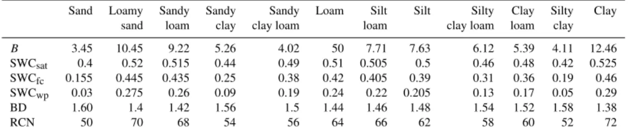
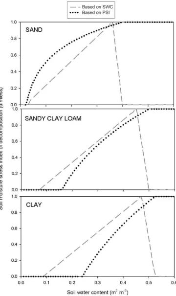
The NSWC and the soil water potential as function of SWC are presented in Fig. 1 for three different soil types: sand soil (sand: 90 %, silt: 5 %), sandy clay loam (sand: 50 %, silt: 20 %), and clay soil (sand: 8 %, silt: 45 %).
According to our definition, SMSI is a function of NSWC and can vary between 0 (maximum stress) and 1 (minimum stress).
Figure 1.Dependence of normalized soil water content (upper part) and soil water potential (lower part) on soil water content in the case of three different soil types. Dimless indicates dimensionless measurements.
The general form of SMSI is defined by the following equations:
SMSI= NSWC
NSWCcrit1, if NSWC<NSWCcrit1
SMSI=1, if NSWCcrit1<NSWC≤NSWCcrit2
SMSI= 1−NSWC
1−NSWCcrit2,if NSWCcrit2<NSWC
, (7)
where NSWCcrit1and NSWCcrit2(NSWCcrit1<NSWCcrit2)
are the characteristic points of the normalized soil water curve, calculated from the soil water potential values or rela-tive soil water content defined by ecophysiological param-eters. Conversion from relative values to NSWC is made within the model. Characteristic point NSWCcrit1is used to control drought-related limitation, while NSWCcrit2 is used to control excess-water-related limitation (e.g., anoxic-soil-related stomatal closure).
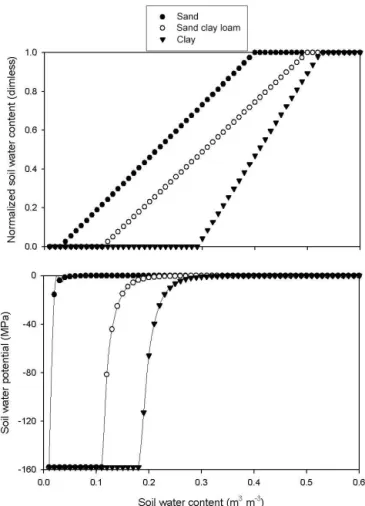
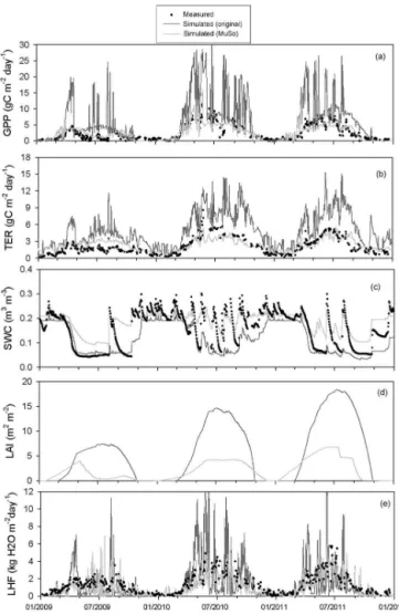
Figure 2.Dependence of the soil moisture stress index on soil water content for three different soil types: sand(a), sandy clay soil(b), and clay(c). Soil stress index based on soil water potential (dotted lines) is used by the original model, while soil stress index based on normalized soil water content is used by BBGCMuSo (dashed lines).
The value of the SMSI is zero in the case of full soil wa-ter stress (below the wilting point). It starts to increase at the wilting point (which depends on soil type; Table 1) and reaches its maximum (1) at the SWC where water stress ends. This latter characteristic value can be set by the user. In this example (Fig. 2), field capacity was used as the character-istic value. The new feature of the BBGCMuSo is that be-yond the optimal soil moisture content range, the soil stress can decrease again (i.e., increasing stress) due to saturation. This second characteristic value (limit2) can also be set by a model parameter. In the example of Fig. 2, 95 % of the satu-ration value was used as the second characteristic value.
Though soil water status is calculated layer by layer, the model requires a single soil moisture stress function to cal-culate stomatal conductance. To satisfy this need, an average stress function for the total root zone is necessary, which is
the average of the layer factors weighted by root fraction in each layer.
Besides stomatal conductance, SMSI is used in the transpi-ration calculation in the multilayer soil. Instead of the aver-aged soil water status of the whole soil column (as in the orig-inal Biome-BGC), in BBGCMuSo, the transpiration flux is calculated layer by layer. The transpiration flux of the ecosys-tem is assumed to be equal to the total root water uptake on a given day (TRPsum). The transpiration calculation is based
on the Penman–Monteith equation using stomatal conduc-tance (this feature is the same as in the original Biome-BGC method). The transpiration fluxes are divided between lay-ers (TRPlayer) according to the soil moisture limitation of
the given layer (SMSIlayer)and the root fraction in the given
layer (Rlayerin Eq. 5):
TRPlayer=TRPsum·SMSIlayer·Rlayer
SMSIsum , (8)
where SMSIsumis the sum of the SMSIlayervalues in the root zone.
According to the modifications, if the soil moisture limita-tion is full (SMSI=0), no transpiration can occur.
4.1.7 Senescence calculation
The original Biome-BGC ignores plant wilting and associ-ated senescence (where the latter is an irreversible process) caused by prolonged drought. In order to solve this problem, a new module was implemented to simulate the ecophysi-ological effect of drought stress on plant mortality. A senes-cence simulation has already been implemented in developed Biome-BGC (Hidy et al., 2012) and it was further improved in BBGCMuSo following a different approach. In BBGC-MuSo, if the plant-available SWC decreases below a critical value, the new module starts to calculate the number of the days under drought stress. Due to low SWC during a pro-longed drought period, aboveground and belowground plant material senescence is occurring (actual, transfer, and stor-age C and N pools) and the wilted biomass is translocated into the litter pool.
A so-called “soil stress effect” (SSEtotal)is defined to
cal-culate the amount of plant material that wilts due to cell death in 1 day due to drought stress. The SSEtotal quantifies the
The SSEtotal varies between 0 (no stress) and 1 (total stress). According to the BBGCMuSo logic, the SSEtotal is the function of SMSI, NDWS, NDWScrit, and SMSIcrit:
SSEtotal =SSESMSI·SSENDWS
SSESMSI=
1− SMSI
SMSIcrit
;if SMSI<SMSIcrit
SSESMSI=0 ;if SMSI≥SMSIcrit
SSENDWS= NDWS
NDWScrit ;if NDWS<NDWScrit
SSENDWS=1 ;if NDWS≥NDWScrit
. (9)
The SEEtotal is used to calculate the actual value of non-woody aboveground and belowground mortality defined by SMCA and SMCB, respectively. SMCA defines the fraction of living C and N that dies in 1 day within leaves and herba-ceous stems. SMCB does the same for fine roots. SMCA and SMCB are calculated using two additional ecophysiologi-cal parameters: minimum mortality coefficient (minSMC) of non-woody aboveground (A) and belowground (B) plant ma-terial senescence (minSMCA and minSMCB, respectively):
SMCA=minSMCA+(1−minSMCA)·SSEtotal
SMCB=minSMCB +(1−minSMCB)·SSEtotal
. (10)
Parameters minSMCA and minSMCB can vary between 0 and 1. In the case of 0, no senescence occurs. In the case of 1, all living C and N will die within 1 day after the occurrence of drought stress. In this sense, SMCA and SMCB can vary between their minimum value (minSMCA and minSMCB, respectively, if SSEtotal is zero) and 1 (if SSEtotalis 1). This latter case occurs when NDWS>NDWScritand SMSI=1.
SMCA is used to calculate the amount of non-woody aboveground plant material (leaves and soft stem) transferred to the standing dead biomass pool (STDB; kgC m−2)due to
soil moisture stress-related mortality on a given day. Note that STDB is a temporary pool from which C and N contents transfer to the litter pool gradually; the concept of STDB is a novel feature in the model. In the case of belowground mor-tality, it defines the amount of fine root that goes to the lit-ter pool directly. The actual senescence ratio is calculated as SMCA (and SMCB) multiplied with the actual living C and N pool.
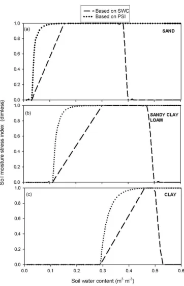
Figure 3 demonstrates the senescence calculation with an example. The figure shows the connections between the change of SWC, normalized soil water content, SMSI, differ-ent types of soil stress effects (SSESMSI, SSENDWS, SSEtotal),
and senescence mortality coefficient as function of number of days since water stress is present. The figure shows a theoret-ical situation in which SWC decreases from field capacity to hygroscopic water within 30 days. The calculation refers to a sandy soil (SWCsat=0.44 m3m−3, SWCfc=0.25 m3m−3,
SWCwp=0.09 m3m−3; SWCfc refers to SWC at field
ca-pacity). In this example, we assumed that relSWCcrit1is 1.0
(field capacity) and relSWCcrit2=0.9 (10 % below
satura-Figure 3.Demonstration of the senescence calculation with an ex-ample.(a)Soil water content (SWC; black dots), normalized soil water content (NSWC; white dots) and soil moisture stress index (SMSI; black triangles) during 30 days of a hypothetical drought event. (b) Soil stress effect based on soil moisture stress index (SSESMSI; black dots), soil stress effect based on number of days since water stress (SSENDWS)and total soil stress effect (SSEtotal). (c)Aboveground senescence mortality coefficient (SMCA).
tion), the critical number of stress days after which senes-cence mortality is complete (NDWScrit)is 30 and the critical
soil moisture stress index (SMSIcrit)is 0.3.
4.1.8 Decomposition and respiration processes
N contents are also calculated layer by layer from the total C and N content of the soil column weighted by the proportion of the total root mass in the given layer.
The maintenance root respiration flux is calculated based on the following equation:
MR(root)=
nr
X
layer=1
Nroot·Rlayer·mrpern·Q
T (soil)layer−20 10
10
!
, (11)
wherenris the number of the soil layers which contain root,
Nroot is the total N content of the soil,Rlayeris the
propor-tion of the total root mass in the given layer, mrpern is an adjustable ecophysiological parameter (maintenance respira-tion per kg of tissue N),Q10 is the fractional change in
res-piration with a 10◦C temperature change, andT(soil)
layeris
the soil temperature of the given layer.
There are eight types of non-N limited fluxes between lit-ter and soil compartments. These fluxes are the function of soil and litter C or N content, soil moisture, and soil temper-ature stress functions. The most important innovation is that total decomposition fluxes are calculated as the sum of par-tial fluxes regarding to the given layer similarly to respiration flux. The soil temperature function is the same as in the orig-inal Biome-BGC. The soil moisture stress function is a lin-ear function of SWC in contrast to a logarithmic function of soil water potential in the original Biome-BGC. A major de-velopment here is that, besides drought effect, anoxic stress is also taken into account because anoxic conditions caused by saturation can affect decomposition of soil organic matter (and thus N mineralization; Bond-Lamberty et al., 2007a). The shape of the modified stress index (SMSIdecomp)is
sim-ilar to the one presented in Bond-Lamberty et al. (2007a). BBGCMuSo uses the following stress index (with values between 0 and 1) to control decomposition in response to changing SWC in a given layer:
SMSIdecomp= SWC−SWChyg
SWCopt−SWChyg,if SWC≤SWCopt
SMSIdecomp= SWCsat−SWC
SWCsat−SWCopt ,if SWCopt<SWC
, (12)
where SWC, SWChyg, and SWCsat is the actual soil water
content, hygroscopic water, and the saturation values of the given soil layer, respectively. SWCoptis calculated from the relative SWC for soil moisture limitation, which is a user-supplied ecophysiological input parameter. The limitation function of decomposition in the original Biome-BGC (based on PSI) and in BBGCMuSo (based on SWC) are presented in Fig. 4.
In the case of the original model, soil stress index starts to increase at −10 MPa (this value is fixed in the model) and
reaches its maximum at saturation. In the case of BBGC-MuSo, soil stress index starts to increase at hygroscopic wa-ter and reaches its maximum at optimal SWC (which is equal
Figure 4.Soil moisture stress index used by decomposition for three different soil types: sand(a), sandy clay soil(b), and clay(c). Soil stress index based on soil water potential (dotted lines) is used by the original model, while soil stress index based on soil water content is used by BBGCMuSo (dashed grey lines).
to the NSWCcrit2from Eq. 7). The new feature of BBGC-MuSo is that after the optimal soil moisture content, soil stress index can decrease due to saturation soil stress (anoxic soil).
4.2 Management modules
The original Biome-BGC was developed to simulate natural ecosystems with very limited options to disturbance or hu-man intervention (fire effect is an exception). Lack of hu- man-agement options limited the applicability of Biome-BGC in croplands and grasslands, but also in managed forests.
mowing modules were already published as part of the de-veloped Biome-BGC (Hidy et al., 2012).
Since the release of the developed Biome-BGC, we im-proved the model’s ability to simulate management. In BBGCMuSo, the user can define seven different events for each management activity, and additionally annually vary-ing management activities can be defined. Further technical information about using annually varying management ac-tivities is detailed in Sect. 3.2. of the user guide (Hidy et al., 2015). Additionally, new management modules were imple-mented and the existing modules were further developed and extended. The detailed description of mowing and grazing can be found in Hidy et al. (2012).
4.2.1 Harvest
In arable crops, the effect of harvest is similar to the effect of mowing in grasslands, but the fate of the cut-down fraction of aboveground biomass is different. We assume that after har-vest, snags (stubble) remain on the field as part of the accu-mulated biomass, and part of the plant residue may be left on the field (in the form of litter typically to improve soil qual-ity). Yield is always transported away from the field, while stem and leaves may be transported away (and utilized, e.g., as animal bedding) or may be left at the site. The ratio of harvested aboveground biomass that is taken away from the field has to be defined as an input.
If residue is left at the site after harvest, the cut-down plant material first goes into a temporary pool that gradually enters the litter pool. The turnover rate of mown/harvested biomass to litter can be set as an ecophysiological parameter. Although harvest is not possible outside the growing season, this temporary pool can contain plant material also in the dor-mant period (depending on the amount of the cut-down ma-terial and the turnover rate of the pool). The plant mama-terial turning into litter compartment is divided between the dif-ferent types of litter pools according to the parameterization (based on unstable, cellulose, and lignin fractions). The wa-ter stored in the canopy of the cut-down fraction is assumed to be evaporated.
4.2.2 Ploughing
As a management practice, ploughing may be carried out in preparation for sowing or following harvest. Three types of ploughing can be defined in BBGCMuSo: shallow, medium, and deep (first; first and second; first, second, and third soil layers are affected, respectively). Ploughing affects the pre-defined soil texture, as it homogenizes the soil (in terms of texture, temperature, and moisture content) for the depth of the ploughing. We assume that due to the plough the snag or stubble turns into a temporary ploughing pool on the same day. A fixed proportion of the temporary ploughing pool (an ecophysiological parameter) enters the litter pool on a given day after ploughing. The plant material turning into the
ter compartment is divided between the different types of lit-ter pools (labile, unshielded cellulose, shielded cellulose, and lignin).
A new feature of Biome-BGCMuSo is that aboveground and belowground (buried) litter is handled separately in or-der to support future applications of the model in cropland-related simulations (presence of crop residues at the surface affects runoff and soil evaporation). As a consequence of lit-terfall during the growing season and the result of harvest, litter accumulates at the surface. In the case of ploughing, the content of aboveground litter turns into the belowground lit-ter pool. In this way, aboveground/belowground litlit-ter amount can be quantified.
4.2.3 Fertilization
The most important effect of fertilization in BBGCMuSo is the increase of mineralized soil nitrogen. We define an actual pool which contains the amount of fertilizer’s nitrogen con-tent put out onto the ground on a given fertilizing day (actual pool of fertilizer; APF). A fixed proportion of the fertilizer enters the top soil layer on a given day after fertilizing. It is not the entire fraction that enters the soil because a given proportion is leached (this is determined by the efficiency of utilization that can be set as an input parameter). Nitrate con-tent of the fertilizer (that has to be set by the user) can be taken up by the plant directly; therefore, we assume that it goes into the soil mineral N pool. Ammonium content of the fertilizer (that also has to be set by the user) has to be nitrified before being taken up by plants; therefore, it turns into the lit-ter nitrogen pool. C content of fertilizer turns into the litlit-ter C pool. As a result, APF decreases day by day after fertilizing until it becomes empty, which means that the effect of the fertilization ends (in terms of N input to the ecosystem). 4.2.4 Planting
In BBGCMuSo, transfer pools are defined to contain plant material as a germ (or bud or nonstructural carbohydrate) in the dormant season from which C and N get to the normal pools (leaf, stem, and root) in the beginning of the subsequent growing season. In order to simulate the effect of sowing, we assume that the plant material which is in the planted seed goes into the transfer pools, thus increasing its content. Al-location of leaf, stem, and root from seed is calculated based on allocation parameters in the ecophysiological input data. We assume that a given part of the seed is destroyed before sprouting (this can be adjusted by the user).
4.2.5 Thinning
or can be left at the site. The rate of transported stem and/or leaf biomass can be set by the user. The transported plant material is excluded from further calculations. The plant ma-terial translocated into coarse woody debris (CWD) or litter compartments are divided between the different types of lit-ter pools according to paramelit-terization (coarse root and stem biomass go into the CWD pool; if harvested stem biomass is taken away from the site, only coarse root biomass goes to CWD). Note that storage and transfer pools of woody har-vested material are translocated into the litter pool.
The handling of the cut-down, non-removed pools dif-fers for stem, root, and leaf biomass. Stem biomass (live and deadwood; see Thornton, 2000 for definition of dead-wood in the case of Biome-BGC) is immediately translocated into CWD without any delay. However, for stump and leaf biomass implementation, an intermediate turnover process was necessary to avoid C and N balance errors caused by sud-den changes between specific pools. The parameter “turnover rate of cut-down, non-removed, non-woody biomass to litter” (ecophysiological input parameter) controls the fate of (pre-viously living) leaves on cut-down trees, and it also controls the turnover rate of dead coarse root (stump) into CWD. 4.2.6 Irrigation
In the case of the novel irrigation implementation, we assume that the sprinkled water reaches the plant and the soil simi-larly to precipitation. Depending on the amount of the water reaching the soil (canopy water interception is also consid-ered) and the soil type, the water can flow away by surface runoff process while the rest infiltrates the top soil layer. Ir-rigation amount and timing can be set by the user.
4.2.7 Management-related plant mortality
In the case of mowing, grazing, harvest, and thinning, the main effect of the management activity is the decrease of the aboveground plant material. It can be hypothesized that due to the disturbance-related mortality of the aboveground plant material, the belowground living plant material also de-creases but at a lower (and hardly measurable) rate. There-fore, in BBGCMuSo we included an option to simulate the decrease of the belowground plant material due to manage-ment that affects aboveground biomass. The rate of the be-lowground decrease to the mortality rate of the aboveground plant material can be set by the user. As an example, if this parameter is set to 0.1, the mortality rate of the belowground plant material is 10 % of the mortality of the aboveground material on a given management day. Aboveground material refers to actual pool of leaf, stem, and fruit biomass while belowground material refers to actual pool of root biomass and all the storage-transfer pools.
4.3 Other plant-related model processes
The original Biome-BGC had a number of static features that limited its applicability in some simulations. In Biome-BGC, we added new features that can support model applica-tions in a wider context, e.g., in climate-change-related stud-ies and modeling exercises comparing free air CO2
enrich-ment (FACE) experienrich-ment data with simulations (Franks et al., 2013).
4.3.1 Phenology
To determine the start and end of the growing season, the phenological state simulated by the model can be used (White et al., 1999). We have enhanced the phenology mod-ule of the original Biome-BGC, keeping the original logic and providing the new method as an alternative. We devel-oped the so-called heat sum growing season index (HSGSI; Hidy et al., 2012), which is the extension of the GSI index proposed by Jolly et al. (2005).
In the original, as well as in the modified Biome-BGC model versions, snow cover did not affect the start of the veg-etation period and photosynthesis. We implemented a new, dual snow cover limitation method in BBGCMuSo. First, the growing season can only start if the snowpack is less than a critical amount (given as millimeters of water content stored in the snowpack). Second, the same critical value can also limit photosynthesis during the growing season (no C uptake is possible above the critical snow cover; we simply assume that in the case of low vegetation, no radiation reaches the surface if snow depth is above a predefined threshold). The snow cover estimation is based on precipitation, mean tem-perature and incoming shortwave radiation (original model logic is used here). The critical amount of snow can be de-fined by the user.
4.3.2 Genetically programmed leaf senescence