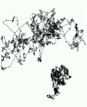
Anomalous diffusion of pions at RHIC

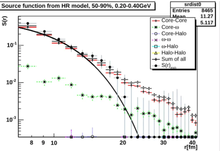
For the data, the statistical uncertainties are indicated as vertical bars, and the combined statistical and systematic uncertainties are shown by the hatched bands.. The

We investigated the diagnostic value of the apparent diffusion coef fi cient (ADC) and fractional anisotropy (FA) of magnetic resonance diffusion tensor imaging (DTI) in patients

Posteriormente, estudou-se as respostas de algumas MNT em estudo quando em condições de privação de nutrientes (água destilada), ao longo de 4 meses, observando-se que as

Na verdade, será questionável até que ponto o Estado não deveria adotar a seguinte estratégia: preferencialmente, impedir que as famílias arrendem habitações

We analyze the event-by-event fluctuations of mean transverse momentum measured recently by the PHENIX and STAR Collaborations at RHIC. We argue that the observed scaling of strength

We analyze experimental data from Pb+Pb collisions at CERN-SPS and Au+Au collisions at BNL-RHIC to determine the amplitude of inhomo- geneities and the role of local and

We have fitted the BRAHMS pseudo-rapidity distributions with the resulting simple forms, and pointed out that in Au+Au collisions at RHIC, 8.5 - 10 GeV/fm 3 initial energy densities

Figure 1. A: Axial magnetic resonance imaging of the skull demonstrating foci of hypersignal at diffusion-weighted sequences in the heads of the caudate nuclei, putamina, thalami