www.atmos-chem-phys.net/12/1737/2012/ doi:10.5194/acp-12-1737-2012
© Author(s) 2012. CC Attribution 3.0 License.
Chemistry
and Physics
Impact of lightning-NO on eastern United States photochemistry
during the summer of 2006 as determined using the CMAQ model
D. J. Allen1, K. E. Pickering2, R. W. Pinder3, B. H. Henderson4, K. W. Appel3, and A. Prados5 1Department of Atmospheric and Oceanic Science, University of Maryland, College Park, MD, USA 2Atmospheric Chemistry and Dynamics Laboratory, Code 614 NASA-Goddard, Greenbelt, MD, USA 3Atmospheric Modeling and Analysis Division, US EPA, Research Triangle Park, NC, USA
4University of North Carolina Chapel Hill, NC, USA
5Joint Center for Earth Sciences Technology (JCET), University of Maryland Baltimore County, Baltimore, MD, USA
Correspondence to:D. J. Allen ([email protected])
Received: 2 May 2011 – Published in Atmos. Chem. Phys. Discuss.: 23 June 2011 Revised: 22 December 2011 – Accepted: 5 February 2012 – Published: 16 February 2012
Abstract.A lightning-nitrogen oxide (NO) algorithm is im-plemented in the Community Multiscale Air Quality Model (CMAQ) and used to evaluate the impact of lightning-NO emissions (LNOx) on tropospheric photochemistry over the United States during the summer of 2006.
For a 500 mole per flash lightning-NO source, the mean summertime tropospheric NO2column agrees with satellite-retrieved columns to within−5 to +13 %. Temporal
fluctua-tions in the column are moderately well simulated; however, the addition of LNOxdoes not lead to a better simulation of day-to-day variability. The contribution of lightning-NO to the model column ranges from∼10 % in the northern US to
>45 % in the south-central and southeastern US. Lightning-NO adds up to 20 ppbv to upper tropospheric model ozone and 1.5–4.5 ppbv to 8-h maximum surface layer ozone, al-though, on average, the contribution of LNOxto model sur-face ozone is 1–2 ppbv less on poor air quality days. LNOx increases wet deposition of oxidized nitrogen by 43 % and total deposition of nitrogen by 10 %. This additional deposi-tion reduces the mean magnitude of the CMAQ low-bias in nitrate wet deposition with respect to National Atmospheric Deposition monitors to near zero.
Differences in urban/rural biases between model and satellite-retrieved NO2 columns were examined to iden-tify possible problems in model chemistry and/or transport. CMAQ columns were too large over urban areas. Biases at other locations were minor after accounting for the im-pacts of lightning-NO emissions and the averaging kernel on model columns.
In order to obtain an upper bound on the contribution of uncertainties in NOy chemistry to upper tropospheric NOx low biases, sensitivity calculations with updated chemistry were run for the time period of the Intercontinental Chemical
Transport Experiment (INTEX-A) field campaign (summer 2004). After adjusting for possible interferences in NO2 measurements and averaging over the entire campaign, these updates reduced 7–9 km biases from 32 to 17 % and 9–12 km biases from 57 to 46 %. While these changes lead to bet-ter agreement, a considerable unexplained NO2low-bias re-mains in the uppermost troposphere.
1 Introduction
Production of nitric oxide (NO) by lightning (LNOx)is an important part of the summertime tropospheric reactive odd nitrogen (NOx= NO + nitrogen dioxide (NO2))budget over the United States, but it is also its most uncertain component. Globally, the LNOxsource is thought to be in the range of 2– 8 Tg N yr−1(Schumann and Huntrieser, 2007). Global model simulations indicate that LNOx increases summertime up-per tropospheric NOxconcentrations over the eastern United States by 60–75 %, upper tropospheric ozone amounts by 15–25 %, and surface ozone concentrations by several ppbv (Zhang et al., 2003; Cooper et al., 2006, 2007; Allen et al., 2010).
Singh et al. (2007) found unexpectedly large amounts of NOx in the upper troposphere during the Intercontinental Chemical Transport Experiment (INTEX-A) field campaign. With few exceptions, modelers have been unable to repro-duce these high NOxamounts, although increasing the mid-latitude lightning-NO source reduces biases (Hudman et al., 2007; Pierce et al., 2007; Bousserez et al., 2007; Choi et al., 2008; Fang et al., 2010; Allen et al., 2010).
years (e.g. Novak and Pierce, 1993), lightning-NO emissions have only been added to regional chemistry and transport models during the last few years (e.g. Kaynak et al., 2008; Smith and Mueller, 2010; Koo et al., 2010). The addition of LNOxwas a relatively low priority because most regional models were developed to serve the air quality community and upper tropospheric processes were considered secondary in importance. However, Napelenok et al. (2008) found that low-biases in upper tropospheric NOx in Community Multiscale Air Quality Model (CMAQ) (Byun and Schere, 2006) simulations without lightning-NO emissions made it difficult to constrain ground-level NOx emissions using in-verse methods and Scanning Imaging Absorption Spectrom-eter for Atmospheric Cartography (SCIAMACHY) (Bovens-mann et al., 1999; Sioris et al., 2004; Richter et al., 2005) NO2retrievals. They also found that wet deposition of nitric acid (HNO3)at National Atmospheric Deposition Program (NADP) sites was underestimated by a factor of two when LNOxwas not included.
Here, the lightning-NO parameterization of Allen et al. (2010) is adapted for use in CMAQ. This module is ex-pected to be available in the next release of CMAQ. This scheme is similar to the schemes of Kaynak et al. (2008), Smith and Mueller (2010), and Koo et al. (2010) in that it uses flash rates from the National Lightning Detection Net-work (NLDN) (Orville et al., 2002) to constrain lightning-NO emissions. This scheme is similar to Koo et al. (2010) in that it places lightning-NO emissions at the locations of model convection. It differs in its vertical partitioning and also because it scales the emissions locally so that monthly average flash rates in each grid cell match NLDN observed flash rates after adjusting for climatological IC/CG ratios.
As part of the evaluation of this scheme, CMAQ simu-lations with and without lightning-NO production are used to estimate the contribution of lightning-NO to upper tropo-spheric photochemistry, surface air quality, and nitrogen de-position over the continental United States for the summer of 2006. The evaluation is the first to use detailed comparisons with in situ and space-based measurements. Finally, in order to obtain an upper bound on the contribution of uncertainties in NOychemistry to upper tropospheric NOxlow biases, sen-sitivity calculations with updated chemistry were run for the time period of the INTEX-A field campaign (summer 2004) in order to determine if lightning-NO and recent improve-ments in our understanding of NOychemistry can lead to a better simulation of the upper tropospheric NOx concentra-tions measured during INTEX-A.
2 Observations and model
2.1 NO2column products from OMI
The Ozone Monitoring Instrument (OMI) aboard the NASA Aura satellite (launched 15 July 2004) measures direct- and
back-scattered sunlight in the ultraviolet-visible range. It re-trieves NO2with a resolution of up to 13 km×24 km. Two
tropospheric NO2 products are used in this study. These products are the DOMINO product (Boersma et al., 2007, 2011) and the DOMINO/GEOS-Chem product (DP-GC) (Lamsal et al., 2010). These products use the same slant column and the same approach for separation of the strato-spheric column from the tropostrato-spheric column. They differ in their calculation of the tropospheric air mass factor. These differences lead to substantially different tropospheric col-umn amounts (e.g. Bucsela et al., 2008; Lamsal et al., 2010; Herron-Thorpe et al., 2010). Version 2.0 (Boersma et al., 2011) of the DOMINO product is used in this study. The DP-GC product differs from version 1.0.2 of the DOMINO prod-uct in that it uses cross-track bias corrected slant columns and calculates its air mass factors using vertical profiles from the GEOS-CHEM model (Martin et al., 2003) rather than the TM4 model (Dentener et al., 2003).
Gridded 0.25◦
×0.25◦DP-GC fields were obtained from
Lamsal et al. (2010). Gridded DOMINO fields were cre-ated by mapping version 2.0 level 2 DOMINO fields onto the same 0.25◦
×0.25◦ grid. On a day-by-day basis,
high-quality DOMINO retrievals with fields of view that partially or totally overlap a given grid box were identified. Re-trievals over snow- and ice-free surfaces with cloud radiance fractions of less than 50 % were identified as high quality (Boersma et al., 2009). The mean value in each grid box was then obtained by weighting the high-quality retrievals using the algorithm of Celarier and Retscher (2009). This algorithm gives more weighting to pixels with near-nadir field of views than far-off-nadir fields of view and to clear pixels than partly cloudy pixels. Pixels with cloud geo-metric fractions exceeding 0.3 are given a weighting of 0. Since lightning-NO emissions are associated with clouds, this cloud-dependent weighting could lead to a low-bias in satellite-retrieved columns. In order to minimize the impact of this effect on conclusions, CMAQ profiles are weighted in the same manner as DOMINO profiles. The mean value in each 0.25◦×0.25◦ grid box was obtained by weighting the
CMAQ profiles using the weights associated with their corre-sponding DOMINO retrievals. When appropriate, the aver-aging kernel was applied to tropospheric model sub-columns before the weighting was performed. Details on the aver-aging kernel processing are given in Allen et al. (2010) and Boersma et al. (2009).
2.2 Ozone profiles from OMI and sondes
fitting residuals exceeding 2 or root mean square (RMS) er-rors exceeding 1.5 are flagged as questionable and are re-moved from the OMI data set. In step two, CMAQ profiles are extracted at the locations and times of the remaining OMI retrievals. CMAQ output is archived hourly. The hours to ex-tract are determined by comparing the local times at CMAQ grid boxes with the Aura satellite overpass time. In step three, these profiles are interpolated onto the OMI vertical grid and converted to Dobson Units. In step four, CMAQ ozone amounts in OMI layers above the CMAQ model top (50 hPa) are set to the OMI a priori. This step is for con-venience only and does not impact the ultimate tropospheric column. In step five, OMI averaging kernels are applied to the CMAQ profiles. In step six, layers within the troposphere are summed to obtain tropospheric columns for each OMI pixel. The OMI tropopause pressure and the number of OMI layers within the troposphere are contained in the OMI data set. The OMI data sets are constructed so that no layer spans the tropopause. The result of these steps is an estimate of the CMAQ tropospheric column at the locations of OMI re-trievals. In step 7, retrievals with cloud fractions exceeding a threshold (50 % here) are removed. The remaining OMI and CMAQ columns for each day are then aggregated onto a 0.5◦
×0.5◦ grid. Each pixel is only assigned to one grid
box using the longitude and latitude at the center of the OMI pixel.
During the summers of 2004 and 2006 as part of the INTEX Ozonesonde Network (IONS), several hundred ozonesondes were launched from North American sites in-cluding Boulder, CO; Houston, TX; Huntsville, AL; and Wallops Island, VA (Thompson et al., 2007a, b). Ozone pro-files from these sondes will be compared to CMAQ propro-files from the same time.
2.3 CMAQ model and simulations
The 2006 simulation without lightning-NO emissions was performed as part of the Air Quality Model Evaluation In-ternational Initiative (AQMEII) (Rao et al., 2010), while the 2006 simulation with lightning-NO emissions was specially performed for the work described in this paper. Both sim-ulations were performed with CMAQ version 4.7.1, Car-bon Bond 2005 (CB-05) chemical mechanism, and AERO5 aerosol module. The model domain included all of the conti-nental United States at 12 km horizontal resolution (459 lon-gitudes by 299 latitudes) with 34 vertical layers from the surface to the 50 hPa model top. Approximately 12 model layers are in the lowest 1-km of the atmosphere. Meteo-rological fields were obtained from a year-long simulation with version 3.1 of the Weather Research and Forecasting Model (WRF) (Skamarock et al., 2005) with the Kain-Fritsch convective parameterization (Kain and Fritsch, 1993). The emissions included data from point sources equipped with continuous emissions monitoring systems (CEMs) that mea-sure sulfur dioxide (SO2)and NOxemission rates and other
parameters daily, mobile emissions processed by the Mo-bile6 model, and meteorologically adjusted biogenic emis-sions from the Biogenic Emission Inventory System (BEIS) (Vukovich and Pierce, 2002) 3.14, all specific for the year 2006. All other emissions are from the National Emission Inventory 2005 version 2, scaled to represent year 2006 (http: //www.epa.gov/ttnchie1/emch/). The emissions were chem-ically speciated, and temporally and spatially allocated us-ing Sparse Matrix Operator Emissions (SMOKE) version 2.6 (SMOKE et al., 2009). Temporally varying chemical bound-ary conditions are from the Global and regional Earth-system (Atmosphere) Monitoring using Satellite and in-situ data (GEMS) (Hollingsworth et al., 2008). The GEMS data are reported every three hours and are interpolated to hourly val-ues for CMAQ. The 2006 simulations were initialized on 22 December 2005 and run through 31 December 2006. The first 10 days of the simulation are excluded from the analysis to remove the influence of initial conditions.
While 2006 offers the opportunity to compare with sur-face and high-resolution satellite-based measurements, prior work has shown that CMAQ underestimates the high NOx concentrations measured in the upper troposphere during INTEX-A in 2004 (Napelenok et al., 2008). Accordingly, in addition to the 2006 simulation described above, the sum-mer of 2004 CMAQ simulations described by Napelenok et al. (2008) are revisited to better understand NOx in the up-per troposphere. For consistency, these simulations use the same modeling domain. It includes the continental United States at 36 km horizontal resolution with 24 vertical lay-ers. Meteorological fields were developed using the fifth generation mesoscale model (MM5) version 3.6.3 (Grell et al., 1995). The emissions are developed for year 2004 us-ing the same data sources as described above; details are available in Gilliland et al. (2008). To take advantage of re-cent developments relevant to the upper troposphere, we use CMAQv4.7.1 with CB-05 chemistry and AERO5 aerosols. Boundary conditions are derived from a GEOS-Chem (Bey et al., 2001) simulation and are spatially variable, but con-stant in time. Upper tropospheric ozone amounts in the 2004 boundary conditions are capped at 75 ppbv. The 2004 sim-ulations were initialized on 21 May 2004 and run through 30 August 2004. The first ten days of the simulation are ex-cluded from the analysis to remove the influence of initial conditions.
2.3.1 Specification of lightning-NO source in CMAQ
CMAQ requires emissions as a function of time and space. The lightning NO source (LNOx)was parameterized in terms of the flash frequency (LF), flash energy (E), and the NO production per unit energy (P). Symbolically,
LNOx=k·LF·E·P , (1)
this equation is the assumption that intracloud (IC) flashes are as energetic as cloud-to-ground (CG) flashes. The flash energy associated with CG and IC flashes has been the subject of much recent research. Recent midlatitude and subtropical storm-scale case studies involving cloud-resolved modeling constrained by observed flash rates and anvil NOx measurements from field experiments such as STERAO (DeCaria et al., 2005), CRYSTAL-FACE (Ott et al., 2007); and EULINOX (Fehr et al., 2004) have found that IC flashes are approximately as energetic as CG flashes and that both CG and IC midlatitude flashes produce approxi-mately 500 moles of N per flash on average (Ott et al., 2010). This value is on the higher end of estimates in Schumann and Huntriesser (2007) and is much higher than a recent top-down estimate obtained by Beirle et al. (2010) from their comparison of observed flash rates and NO2columns from SCIAMACHY. In these CMAQ simulations, we assume all flashes produce 500 moles of N. The LNOx algorithm we have developed for CMAQ ensures that lightning emissions are located only in grid cells in which parameterized deep convection is active. The flash frequency for each grid box is obtained by multiplying domain-wide (D) and local (αi,j) scaling factors by the adjusted convective precipitation rate. Symbolically,
LFi,j=D·αi,j·(preconi,j−threshold)γ, (2) wherei andj are indices of individual CMAQ grid boxes, precon is the convective precipitation rate from the meteoro-logical model at grid boxes where the convective cloud top pressure is less than 450 hPa (i.e. deep convection), threshold is the value of precon below which the flash rate is assumed to equal zero,Dis a scaling factor chosen so that the domain-averaged model flash rate equals a specified value,αis a lo-cal adjustment factor lo-calculated afterD and chosen so that the monthly average model-calculated flash rate for each grid box equals a specified value (e.g. Allen et al., 2010; Martini et al., 2011). The threshold is set to 0 for these simulations because for a pressure threshold of 450 hPa, the mean spatial coverage of deep convection in the meteorological model is less than the mean spatial coverage of lightning flashes. The value for the power (γ ) is set to one because observations over the southern United States show a weak linear relation-ship between flash rate and convective rainfall rate (Petersen and Rutledge, 1998; Tapia et al., 1998). Convective precip-itation was chosen as the flash rate predictor because of this relationship and also because it is readily available in out-put streams from WRF, the meteorological model most com-monly used to drive CMAQ. Tost et al. (2007) examined the performance of other possible predictors including cloud top height and updraft velocity.
Sauvage et al. (2007) and Allen et al. (2010) use time-averaged flash rates from Optical Transient Detector and Lightning Imaging Sensor (OTD/LIS) (Mach et al., 2007) to constrain model flash rates. Martin et al. (2007) use satellite-retrieved trace gas distributions to constrain model
flash rates. In this study, we follow a similar approach but use monthly average flash rates from the National Lightning Detection Network (NLDN) (Cummins et al., 1998) to con-strain model flash rates. Jourdain et al. (2010) used daily average NLDN flash rates to constrain model flash rates. For these simulations the domain-wide constraint (D) is chosen so that when averaged over a month, the domain-averaged flash rate calculated from Eq. (2) withα(i, j) = 1 matches the mean “observed” flash rate. The mean “observed” flash rate over the United States is obtained by mapping detection efficiency-adjusted NLDN flash rates onto the CMAQ grid and then multiplying the resulting flash rates byZ+ 1, where Z is the smoothed climatological IC/CG ratio at that grid box. Unsmoothed climatological values ofZ are available from Boccippio et al. (2001). In order to lessen the differ-ence between 12-km and 36-km local scaling factors and to partially compensate for positioning errors in the location of model convection, the 12-km flash rates are smoothed by a 3×3 moving average before calculatingDandα. NLDN
de-tection efficiencies were obtained from the Vaisala dede-tection efficiency model (R. Holle, personal communication, 2010) but are constrained to be between 0.1 and 0.93, where 0.93 is the estimated detection efficiency of the NLDN over the United States during the 2004–2006 time period (Biagi et al., 2007). Flash rates at locations with NLDN detection effi-ciencies of<10 % are replaced by climatological flash rates from version 2.2 of the OTD/LIS climatology (Boccippio et al., 2002; Mach et al., 2007).
Local adjustment factors (αi,j)are chosen so that when av-eraged over one-month periods of interest, model flash rates match observed total (sum of CG + IC) flash rates subject to the constraint thatαi,j is constrained to be between 0.1 and 10. During non-winter months, the lower constraints are in-voked at approximately 7 % of grid boxes within the 110◦–
70◦W 25◦–45◦N analysis region, while upper constraints
are invoked at approximately 2 % of grid boxes. Therefore, monthly average model flash rates will not exactly match “observed” flash rates. Diurnal and day-to-day fluctuations in flash rates are not constrained.
1
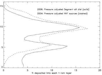
Fig. 1. Vertical distribution of lightning-NO production assumed for 2004 (dashed) and 2006 (solid) simulations. The distribution for 2004 was derived from the vertical distribution of VHF sources in the vicinity of the Northern Alabama LMA during the April to September 2003–2005 time period. The distribution for 2006 was derived from the vertical distribution of segment altitude distribu-tions in the same area.
bit less NO near the intracloud flash generated peak in the upper troposphere and a bit more NO near the peak in the mid-troposphere.
2.3.2 Evaluation of flash rate distribution in CMAQ
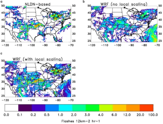
Figure 2a–c compares model and observed 24-h average flash rates on 10 July 2006. On this particular day, light-ning is evident over much of the United States with local maxima over Oklahoma, the Great Lakes, the northeastern United States, and the western Atlantic off the coast of North Carolina. The western Atlantic peak is likely underestimated by the NLDN network as the network is land-based and de-tection efficiencies fall off rapidly more than 300 km from the coast. Model flash rates forαi,j= 1 (Fig. 2b) are similar to observed flash rates although the Oklahoma maximum is shifted northward to Kansas, and the flash frequency is un-derestimated over the Great Lakes and northeastern United States and overestimated over the western Atlantic. Apply-ing the local scalApply-ing factors improves the agreement with ob-servations as flash rates are increased over Oklahoma and the Great Lakes and decreased over the western Atlantic (Fig. 2c).
In order to assess the agreement between modeled and observed flash rates, NLDN flash rates during June-August were matched with model convection. This analysis showed that when averaged over a one-hour time period 35–45 % of the strikes measured by the NLDN occur within WRF grid boxes with convective precipitation. When the averaging pe-riod is increased to one day, more than 90 % of the strikes occur in WRF grid boxes with convective precipitation (not shown). Figure 3a–d summarizes the agreement between
modeled and observed flash rates over the entire domain. Correlations between modeled and observed hourly flash rates average 0.70 and do not vary much from month to month ranging from 0.50 in April 2006 to 0.83 in Decem-ber 2006 (Fig. 3a). The relatively small variability in hourly flash rate correlations from month-to-month masks substan-tial seasonal differences in how well the model captures diur-nal (Fig. 3b) – and daily (Fig. 3c) – fluctuations in the hourly flash rates. Diurnal variations (each hour averaged over a month) are extremely well captured during the summer as di-urnal correlations exceed 0.85 during June through Septem-ber. Reasonable agreement is also seen in transition months with correlations ranging from 0.45 to 0.80 during the spring and fall. Wintertime diurnal correlations vary greatly equal-ing 0.82 in December, 0.31 in January, and−0.02 in
Febru-ary. The larger wintertime variability in monthly correlations is likely due to the weak diurnal cycle during this season and the limited number of events.
During the fall through spring, most thunderstorms occur in the warm sector in advance of a cold front. Day-to-day variations in the locations of these storms are well captured with correlations averaging 0.80 and ranging from 0.67 to 0.90. In the summer, thunderstorms are more stochastic in nature and are difficult to model accurately. Observed and modeled daily-total flash rates are only weakly correlated during this period. The low correlations during this time period mean that the simulation of day-to-day variations in summertime upper tropospheric NO2is unlikely to improve when lightning-NO is added to CMAQ. Day-to-day variabil-ity in flash rates is well captured during fall through mid-spring but underestimated by approximately 30 % during the summer (Fig. 3d).
Correlations between model and observed flash rates are often less than one might hope because of several factors. (1) Lightning is not always associated with convective precipita-tion. (2) The linear dependence of flash rate on convective precipitation rate is an oversimplification. (3) Model convec-tive events, even when simulated, are often misplaced by a few hours or a few grid boxes. As noted before, diurnal errors are largest when diurnal forcing is weak (October–February) and day-to-day errors are largest when synoptic forcing is weak (summer).
3 Results
1
Fig. 2.Flash rate distribution on 10 July 2006.(a)NLDN-based estimate obtained by multiplying NLDN CG flash rate byZ+ 1, whereZis the smoothed climatological IC/CG ratio,(b)model flash rate before applying local-scaling factors, and(c)model flash rate after applying local-scaling factors
for determining the response of ozone to NOxperturbations of less than 30–40 % (Kunkrishnan and Lawrence, 2004), and it may be the best approach for determining the amount of ozone with a lightning-NO source (e.g. Hudman et al., 2007; Sauvage et al., 2007b; Kaynak et al., 2008; and Zhao et al., 2009).
Four simulations are performed for 2004 – without light-ning NO (simulation noL), with lightlight-ning NO (simula-tion LNOx), with lightning NO and aircraft NO (simula-tion airLNOx), and a chemistry sensitivity test with up-dates as recommended by Henderson et al. (2011) (simu-lation adjchemLNOx). Aircraft NO emissions for simula-tion airLNOx are based on scheduled commercial aircraft (Baughcum et al., 1996) and military, chartered and non-scheduled jet aircraft (Metwally, 1995) emission inventories developed for the year 1992. For this chemistry sensitivity test, organic nitrate (ON) yield from the oxidation of paraf-fins (PAR) was reduced from 15 % to 3 %. In the CB-05 chemical mechanism, acetone is lumped with the paraffins. Since acetone is a major component (∼75 %) of PAR in the
upper troposphere, this reaction should produce much less ON. The decrease in ON production reduces NO consump-tion, increases the NOxlifetime, and is in better agreement with observations and other models (Henderson et al., 2011).
3.1 Comparison with NO2columns
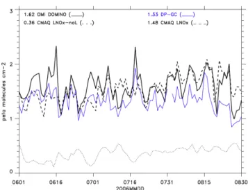
Figure 4 compares model-calculated and satellite-retrieved variations in the mean daily tropospheric NO2column over the eastern two-thirds of the United States and adjacent western Atlantic (110◦–70◦W, 25◦–45◦N). Model columns
were created by integrating model concentrations at the hour closest to the Aura overpass (13:30 LT) from the surface to tropopause. When averaged over the entire time pe-riod, the mean averaging-kernel processed CMAQ column has a small high-bias (11 %) with respect to the mean DP-GC column (1.33 peta molecules cm−2) and a small
low-bias (9 %) with respect to the mean DOMINO column (1.62 peta molecules cm−2). Day-to-day variations in the column are sensitive to the method used to map columns onto a level 3 grid as the temporal correlation between the DOMINO and DP-GC products is only 0.29. The correlation between CMAQ and the DOMINO product is 0.47, while the correlation between CMAQ and the DP-GC product is a relatively robust 0.79. The modest (but non-zero) corre-lations suggest that the model has some skill in capturing day-to-day variations in mean tropospheric column over the United States. For a 500 mole per flash source, lightning-NO emissions on average in the summer of 2006 contributed 0.36×10¹⁵molecules cm−2to the tropospheric column,
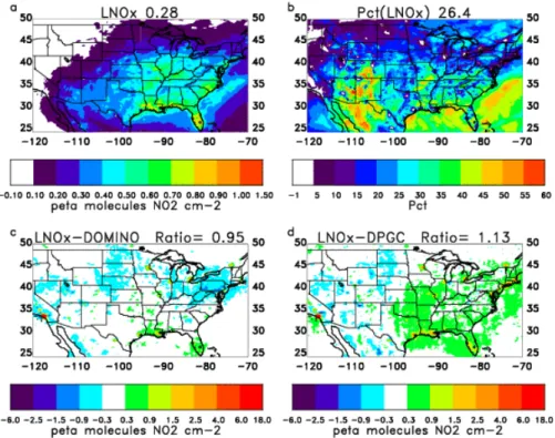
ac-counting for 25 % of the total model column over this region. Figure 5a shows the model-calculated contribution of lightning-NO emissions to the mean tropospheric NO2 column during the summer of 2006. As expected, the contribution is largest over the southeastern United
1
Fig. 4. Time series comparing area-averaged (110◦–70◦W, 25◦–
45◦N) tropospheric NO
2 columns for June–August 2006. Solid
blue (black) line shows the mean DP-GC (version 2.0 DOMINO) column. The dashed line shows averaging-kernel processed model output from simulation LNOx. The dotted line shows the
contribu-tion of lightning-NO produccontribu-tion to the total model column (simula-tion LNOx– simulation noL).
States where lightning is common. Contributions exceed 0.6×10¹⁵molecules cm−2throughout much of Florida and
coastal sections of the southeast. The spatial distribution of percent contributions (Fig. 5b) is much different. It shows peaks over the southwestern United States/northwestern Mexico, the northern Gulf of Mexico, and the western At-lantic (southeast of Virginia). Figure 5c–d shows the biases between the modeled and satellite-retrieved columns. Over-all, the mean column is 5 % low with respect to the DOMINO column but 13 % high with respect to the DP-GC column. With the exception of urban areas, model biases over the western United States are usually negative, while biases over the southern and eastern United States are often positive, es-pecially over extreme southern Louisiana and Florida. Over the northeastern United States, CMAQ has a low-bias with respect to the DOMINO product and a high-bias with respect to the DP-GC product.
Fig. 5. Contribution of lightning-NO to mean tropospheric NO2columns during the summer of 2006 and column biases with respect to
satellite-retrieved columns. The upper left panel shows the increase in NO2column due to LNOx(peta molecules cm−2). The upper right
panel shows the percent of NO2column with an LNOxsource. The lower left (right) panel shows the bias between the averaging kernel
processed NO2column from simulation LNOxand the DOMINO (DP-GC) column.
2
Fig. 6. Mean tropospheric NO2column for 1 June 2006 to 30 August 2006. The upper left panel shows the mean version 2.0 DOMINO column. The upper right panel shows the mean CMAQ column from simulation LNOxon the native 12-km grid. The lower left (right) panel
shows the mean CMAQ column from simulation LNOxon the 0.25◦×0.25◦DOMINO grid without (with) processing by the averaging
application of the OMI DOMINO averaging kernel to model output reduced columns over urban areas in the northwestern United States by 35–50 %. Second, both mapping and aver-aging kernel processing smooth the columns improving the agreement with the satellite-retrieved DOMINO product that has also been mapped onto a 0.25◦×0.25◦grid.
Huijnen et al. (2010) compared tropospheric NO2columns over Europe from ten different regional models and two global models to the DOMINO product, version 1.0.2. They found that median model columns were too low at rural locations and too high at urban locations. Castellanos et al. (2011) also found high biases at urban locations and local biases at rural locations when comparing compared CMAQ-calculated NOy-HNO3 with “NO2” measurements at rural and urban monitoring sites over the eastern United States. These differing biases are important because they suggest that the lifetime of NO2(see Henderson et al., 2011) and/or the transport of NOx(see Gilliland et al., 2008) is underes-timated by regional models. These underestimations could lead to errors in inverse-based emissions of sources and to misleading results as to the relative importance of local ver-sus regional emissions.
In order to investigate this possible problem in more detail, we examine how urban to rural ratios change when lightning-NO emissions are set to zero, when the CMAQ output is mapped onto a 0.25◦
×0.25◦ grid, and when an averaging
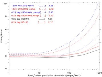
kernel is applied. The resulting ratios are compared to ratios from the DOMINO and DP-GC products. Figure 7 shows these ratios as a function of the population density thresh-old chosen to separate rural sites from urban sites. Pop-ulation data obtained from 2000 census. Only populated United States grid boxes used when calculating the mean ra-tios. In general, model-calculated urban-to-rural ratios ex-ceed satellite-retrieved ratios with differences becoming in-creasingly large as the minimum population density required to be classified as urban increases. The largest urban-to-rural ratios are seen when the analysis is performed using CMAQ output from simulation noL (e.g. 4.05 for a threshold of 100 people per km2). NO2with a lightning-NO source is present over both urban and rural locations. Therefore, the addition of lightning-NO emissions to a CMAQ simu-lation decreases the ratios resulting in slightly better agree-ment with satellite-retrieved values. Ratios decrease substan-tially when the 12-km CMAQ output is mapped onto the 0.25◦
×0.25◦ DOMINO grid (e.g. 2.45 for a threshold of
100 people per km2) because urban grid boxes are mixed with rural grid boxes during the aggregation process. Model-calculated ratios are lowest when Model-calculated with averaging-kernel processed output from simulation LNOx. In this case, differences between model-calculated and satellite-retrieved ratios are only apparent when the population threshold ap-proaches 1000 people per km2 (i.e. when large cities such as Los Angeles or Minneapolis are classified as urban and everything else is classified as rural, see map of biases in Fig. 6).
1
2 Figure 7.Ratio between mean urban and rural tropospheric NO columns as a function of
Fig. 7. Ratio between mean urban and rural tropospheric NO2 columns as a function of the population threshold (people km−2)
used to separate rural and urban grid boxes. The solid black (red) line shows the ratio calculated from the gridded 0.25◦×0.25◦
DOMINO (DP-GC) product. The dashed blue (red) line shows the ratio based on 12-km CMAQ output from simulation noL (LNOx).
The dotted blue (red) line shows the ratio based on CMAQ sim-ulation LNOx output without (with) application of the averaging
kernel.
Three factors contribute to the smearing of urban and ru-ral profiles in the DOMINO product. (1) Mean model (and presumably actual) urban to rural NO2ratios are largest in the surface layer (approximately 6 for a threshold of 100 people km−2)and decrease rapidly with height, equaling 4 at 1 km, 2 at 2 km, and 1.5 at 3.5 km. OMI underestimates these ratios because it is relatively insensitive to the low-est km of the atmosphere. (2) The DOMINO NO2 profile shapes were obtained from a 3◦
×2◦ simulation with the
TM4 model (Boersma et al., 2007). Surface albedos come from a fairly coarse satellite-based climatology. Both of these variables enter into the air mass factor calculation. The use of these relatively coarse profiles and albedos smears ur-ban and rural locations. (3) The footprint of DOMINO pixels is 13×24 km at nadir but increases as the viewing zenith
an-gle (VZA) increases.
product for comparison with model output from the GEOS-Chem model.
To summarize, CMAQ columns in urban areas are bi-ased high with respect to OMI retrievals. However, in gen-eral, most of the differences between modeled and satellite-retrieved urban to rural ratios are likely a consequence of the horizontal and vertical smoothing inherent in the OMI-retrieved columns. These differences are exacerbated when model profiles differ substantially from priori profiles (see also Huijnen et al., 2010). These results highlight the im-portance of using averaging kernels when interpreting differ-ences between model and satellite-retrieved columns.
3.2 Comparison with ozone profiles and columns
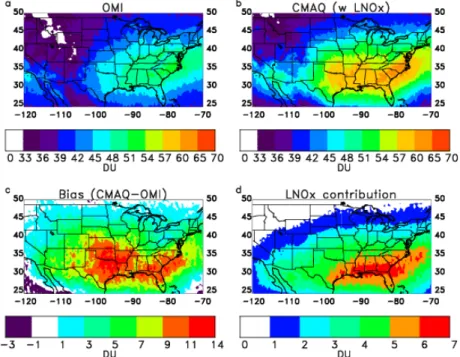
Figure 8a and b compares the mean summer 2006 tropo-spheric columns of ozone from OMI and CMAQ. The mean columns at each grid box were calculated using output from days when OMI measurements were available. Retrievals (and model output at same location) with cloud fractions ex-ceeding 0.5 are not included in the averages. Overall, the spatial distribution of the CMAQ columns is similar to the spatial distribution of the OMI columns; however, the CMAQ columns for the simulation with lightning-NO production are 0–5 % higher than the OMI columns over the northern United States and 10–20 % higher than the OMI columns over the southern United States. High-biases of 9–11 DU with re-spect to the OMI product are common in a region extending from the southern Great Plains to the southeastern United States (Fig. 8c). The bias is not primarily due to an overesti-mation of lightning-NO production as the lightning-NO con-tribution (Fig. 8d) shows a southeastern United States peak and equals only 3–5 DU over the southern Great Plains. The amount of vertical information contained in the OMI tropo-spheric columns is minimal; however, it does suggest that the CMAQ bias with respect to OMI is larger in the upper troposphere than the lower troposphere. Averaged over the region shown in Fig. 8 (25◦–50◦N, 120◦–70◦W), CMAQ
biases in the two lowest OMI layers (from the surface to ap-proximately 500 hPa), which contain 46 % of the OMI tro-pospheric column during this time period equal 4 % while biases in the upper two to four layers equal 20 %. By compar-ison, the one sigma solution errors for OMI at these altitude ranges is 15–20 % (Liu et al., 2010).
Figure 9 compares mean modeled and observed ozone pro-files at IONS sites during the summer of 2006. Lightning-NO production increases model-calculated upper tropo-spheric (7–12 km) ozone by 14–19 ppbv over the Houston, Huntsville, and Wallops, Island sites. Compared to the IONS network, the upper tropospheric ozone concentration simu-lated by CMAQ has very little bias at stations near the west-ern boundary (not shown), but this bias increases for stations in the East. Biases shown here range from 6–8 ppbv at Boul-der and Houston to 26–27 ppbv at Huntsville and Wallops Island.
Simulations of upper tropospheric ozone are sensitive to the rate of vertical mixing. If the mixing rate is too vigor-ous, high ozone concentrations near the stratosphere will be transported downward in excess. This causes the model to overestimate the ozone concentration in the mid and upper troposphere. As air masses move from west to east with the prevailing winds, the excessive vertical mixing increases the bias. This excess ozone can influence the CMAQ calculation of the ozone attributable to lightning NO. To test the impact of this excess ozone, a box model is initialized with observa-tions from INTEX to simulate upper tropospheric chemistry immediately after lightning events (Henderson et al., 2011). Initializing the box model with 20 % additional ozone causes a 10–20 % decrease in ozone production, depending on the level of NOx. Therefore, the ozone production attributable to lightning NO is likely to be larger than the CMAQ estimate by 10–20 %.
3.3 Impact on surface layer ozone
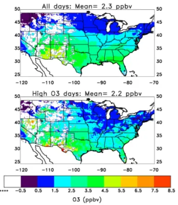
For a lightning-NO emission rate of 500 moles per flash, lightning-NO is responsible for∼25 % of the modeled
sum-mertime tropospheric NO2column (Fig. 5). The mean con-tribution of LNOx to surface layer ozone during the same time period is 2.3 ppbv or∼3 % (Fig. 10a). Over the eastern
United States, mean contributions are typically 0.5–2.5 ppbv in the north and 2.5–4.5 ppbv in the south. Mean contribu-tions in the southwestern United States exceed 3.5 ppbv at many locations with the largest contributions evident over western Texas, New Mexico, Arizona, and Nevada. The rel-atively high impact of LNOxover the southwestern United States is due to a combination of meteorological and photo-chemical factors. Flash rates over the southwestern United States are large during July and August due to the North American monsoon. Sunny conditions in this region enhance ozone production and ozone often mixes to the surface due to the high boundary layer heights over the southwest.
Fig. 8. Mean tropospheric ozone column for 1 June 2006–30 August 2006. Upper left: OMI data, upper right: CMAQ simulation LNOx
after applying averaging kernel, lower left: bias between averaging kernel processed CMAQ simulation LNOxand OMI data, and lower
right: lightning-NO contribution to model column (determined without averaging kernel).
2
3 Figure 9. Mean vertical distribution of ozone at IONS sites during the summer of 2006.
Fig. 9. Mean vertical distribution of ozone at IONS sites during the summer of 2006. Results are shown for Boulder, CO (upper left), Houston, TX (upper right), Huntsville, AL (lower left), and Wallops Island, VA (lower right). CMAQ simulation noL (LNOx)is shown
Table 1. Mean percent of CMAQ grid box-days for which lightning-NO emissions contribute less than1O3ppbv to 8 h maximum ozone
values over the western (longitudes west of 100◦W) and eastern (longitudes east of 100◦W) United States during the 1 June 2006 through
31 August 2006 time period. Only populated CMAQ grid boxes within the conterminous United States are used in the calculation. Means are shown for all grid box days and for grid box days with poor air quality. Air quality is considered poor if 8-h maximum ozone from simulation noL on that day exceeds 60 ppbv in that grid box and that value is among the ten highest values at that grid box during the summer. A grid-box day refers to one grid box on one particular day.
Western United States Eastern United States
1O3 % (All Days) % (Poor AQ days) % (All Days) % (Poor AQ days)
<0.5 37 22 22 18
<1.5 56 47 52 60
<2.5 68 64 68 80
<3.5 76 74 78 88
<4.5 82 81 85 92
<5.5 86 86 90 95
<6.5 90 90 93 97
<20 100 100 100 100
Fig. 10. Mean increase in 8-h maximum ozone associated with lightning-NO production during the 1 June through 31 August time period. Results averaged over all days (top) and over days when 8-h maximum ozone from simulation noL exceeds 60 ppbv (bottom).
and far western Texas) and decrease at some locations (e.g. Kansas, Oklahoma, and Colorado). Overall, 36 % of west-ern United States grid boxes show contributions exceeding 2.5 ppbv on poor air quality days. Lightning-NO emissions are a substantial contributor (>6.5 ppbv) to 8-h maximum
ozone at approximately 10 % of grid points over the west-ern United States and 7 % of grid points over the eastwest-ern United States, although the percent of eastern United States grid points with substantial LNOx impacts falls to 3 % on poor air quality days.
3.4 Impact on deposition of nitrogen species
Table 2 compares the relative contribution of wet and dry processes to the deposition of nitrate and ammonium in the CMAQ model during the June–August 2006 time period. For simulations with lightning-NO emissions, dry and wet depo-sition processes are of equal importance with total depodepo-sition equaling 0.40 g N ha−1h−1for both processes. The relative
contribution of nitrate and ammonium to total deposition is sensitive to lightning-NO emissions. For simulations with lightning-NO production, total deposition of nitrate exceeds total deposition of ammonium by∼25 %. Differences
be-tween the magnitude of nitrate and ammonium deposition are minor for simulations without LNOx. Overall, wet depo-sition of nitrate increases by 43 % when lightning-NO emis-sions are added, while wet deposition of ammonium is virtu-ally unchanged. The 43 % increase in the wet deposition of nitrate corresponds to a 19 % increase in the total deposition of nitrate and a 10 % increase in the total deposition of total nitrogen.
Table 2.Mean dry and wet deposition of nitrate, ammonium, and total nitrogen (N) for June–August 2006 time period from CMAQ simu-lations without (noL) and with (LNOx)lightning-NO production. Results are obtained by averaging model output over region encompassed
by 120◦–70◦W and 25◦–50◦N. Units are g N ha−1h−1.
Drydep Wetdep Totdep Drydep Wetdep Totdep noL noL noL LNOx LNOx LNOx
Nitrate 0.23 0.14 0.37 0.24 0.20 0.44 Ammonium 0.16 0.20 0.36 0.16 0.20 0.36 Total nitrogen 0.39 0.34 0.73 0.40 0.40 0.80
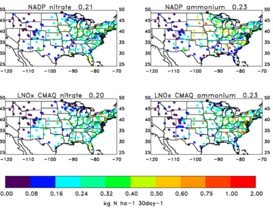
of nitrate equal approximately 0.2 kg N ha−130 day−1 and
modeled and measured deposition of ammonium equal 0.23 kg N ha−130 day−1. Regionally, mean wet deposition of nitrate is overestimated by 8 % in the northeastern United States and by 20–30 % in the southeastern and south cen-tral United States. Wet deposition is slightly underestimated over the rest of the United States (i.e. states in Midwest/Great Plains, Rocky Mountain/West). Regional variations in wet deposition of ammonium are larger. Once again, biases are positive in the eastern United States (∼40 % at
southeast-ern states and∼20 % at northeast states) and negative in the
western United States (low biases of 20–25 %).
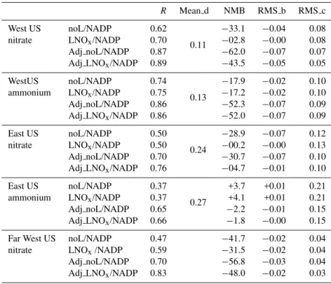
Figure 12 contains scatterplots comparing monthly av-erage modeled and measured wet deposition of nitrate at NADP sites over the western (locations west of 100◦W)
and eastern (locations east of 100◦W) United States. When
lightning-NO emissions are not included, mean deposition rates are biased low at western and eastern sites by 33.1 % and 28.9 %, respectively. When lightning-NO emissions are included the biases are reduced to near zero (−2.8 %
at western sites and −0.2 % at eastern sites). The
impor-tance of LNOx was expected at eastern sites but is some-what surprising at western sites. Closer examination re-veals that less LNOx is needed to reduced NMBs at west-ern sites as the mean deposition rates at westwest-ern sites equal 0.11 kg N ha−130 day−1while mean deposition rates at
east-ern sites equal 0.24 kg N ha−130 day−1. In addition, the
bulk of the improvement at western sites occurs east of the Rockies. Wet deposition of nitrate at far western locations (west of 110◦W) is underestimated by 41.7 % in simulation
noL and 31.5 % in simulation LNOx(Table 3). Wet deposi-tion of ammonium is underestimated by 17.2 % at western sites and overestimated by 4.1 % at eastern sites (see Ta-ble 3). Lightning-NO emissions have minimal impact on these biases.
Correlations between modeled and measured wet depo-sition rates at western locations equal 0.70 for nitrate and 0.75 for ammonium (Table 3). Correlations at eastern sites are lower equaling 0.50 and 0.37, respectively. The lower correlations at eastern sites are likely due to a poorer simu-lation of week-to-week variations in summertime precipita-tion at those locaprecipita-tions. Table 3 also shows correlaprecipita-tions after adjusting for biases in model precipitation. As part of this
adjustment, model precipitation totals at NADP sites are re-placed by observed precipitation totals at NADP sites. When these adjustments are made, correlations between modeled and measured wet deposition rates increase at both western (0.70 to 0.89 for nitrate and 0.75 to 0.86 for ammonium) and eastern sites (0.50 to 0.76 for nitrate and 0.37 to 0.66 for am-monium). Unfortunately, adjusting the precipitation at west-ern sites, introduces large negative wet deposition biases of 43 % (52 %) for nitrate (ammonium). Biases at eastern sites change only slightly after adjusting for biases in precipita-tion, ranging from−4.7 % for nitrate to−1.8 % for
ammo-nium. The large degradation at western sites when precipi-tation rate are adjusted, indicates that the small biases seen at these locations are due to compensation between overes-timated model precipitation rates and underesoveres-timated model deposition efficiency.
3.5 Sensitivity of upper tropospheric NOxand O3to
uncertainties in NOychemistry
1
Fig. 11.Summer 2006 wet deposition of nitrogen at NADP/NTP sites. Upper left: nitrate measurements, upper right: ammonium measure-ments, lower left: nitrate from simulation LNOx, and lower right: ammonium from simulation LNOx.
Fig. 12. Scatterplots comparing modeled and measured wet deposition of nitrate at NADP/NTN sites west of 100◦W (top) and east of
100◦W (bottom). Model results are shown for simulation noL (left) and LNOx(right). Text within each plot shows the correlation (R), the
Table 3.Thirty-day average wet deposition of nitrate and ammonium from the NADP network, CMAQ simulation noL, and CMAQ simula-tion LNOxare compared for June–August 2006. Results are shown for the western United States (average of 136 months at 65 sites located
west of 100◦W), eastern United States (average of 397 months at 160 sites east of 100◦W), and the far-western United States (nitrate only)
(average of 43 months at 25 sites west of 110◦W). The “Adj ” rows show the comparison when the CMAQ precipitation rates are replaced
by the NADP precipitation rates when calculating the deposition rates. From left to right the columns show the region of interest, the data sets compared, the correlation coefficient, the mean of the NADP measurements (kg of N ha−130 days−1), the normalized mean bias, the
bias, and the root mean square error after subtracting the bias.
R Mean d NMB RMS b RMS c West US noL/NADP 0.62
0.11
−33.1 −0.04 0.08
nitrate LNOx/NADP 0.70 −02.8 −0.00 0.08
Adj noL/NADP 0.87 −62.0 −0.07 0.07
Adj LNOx/NADP 0.89 −43.5 −0.05 0.05
WestUS noL/NADP 0.74
0.13
−17.9 −0.02 0.10
ammonium LNOx/NADP 0.75 −17.2 −0.02 0.10
Adj noL/NADP 0.86 −52.3 −0.07 0.09
Adj LNOx/NADP 0.86 −52.0 −0.07 0.09
East US noL/NADP 0.50
0.24
−28.9 −0.07 0.12
nitrate LNOx/NADP 0.50 −00.2 −0.00 0.13
Adj noL/NADP 0.70 −30.7 −0.07 0.10
Adj LNOx/NADP 0.76 −04.7 −0.01 0.10
East US noL/NADP 0.37
0.27
+3.7 +0.01 0.21 ammonium LNOx/NADP 0.37 +4.1 +0.01 0.21
Adj noL/NADP 0.65 −2.2 −0.01 0.15
Adj LNOx/NADP 0.66 −1.8 −0.00 0.15
Far West US noL/NADP 0.47 −41.7 −0.02 0.04
nitrate LNOx/NADP 0.59 −31.5 −0.02 0.04
Adj noL/NADP 0.70 −56.8 −0.03 0.04
Adj LNOx/NADP 0.83 −48.0 −0.02 0.03
The primary aircraft used during INTEX-A was NASA’s DC-8, and one-minute merge data sets are available for all species measured aboard the DC-8. We compared CMAQ output with these measurements after removing one-minute periods when contributions from fresh pollution, biomass burning, or stratosphere-troposphere exchange were greatly enhanced (see Allen et al., 2010, for methodology) Sam-ples with greatly enhanced fresh pollution or biomass burn-ing were removed as they are likely unrepresentative of the 36-km CMAQ grid box. Samples with a greatly enhanced stratospheric contribution were removed because this study focuses on the upper troposphere. Unlike Allen et al. (2010), we did not have tropopause pressure information from the meteorological model and were unable to use that parameter as an additional stratospheric filter.
Figure 13 shows the contribution of LNOx to NO2 dur-ing DC-8 flight 4 of INTEX-A. The DC-8 measured increas-ingly high NOxamounts in the upper troposphere during the latter portion of the flight as the DC-8 moved across Illi-nois, Michigan, and Indiana. Ozone amounts also increased over this region (see Fig. 14). CMAQ simulation LNOxalso showed high amounts of NO2and relatively high amounts of
Fig. 13. Curtain plot comparing model NO2as a function of time (EST) and pressure (hPa) with measurements from DC-8 Flight 4 on
6 July 2004. Top (bottom) panel shows results from simulation noL (LNOx). Measured values are shown with a ribbon. Model values are
shown in the background. The location and time of INTEX-A samples are shown on the United States map. The color bar shows the time of one-minute average samples and the scale for the NOxmeasurements.
Table 4. Mean upper tropospheric (Pressure<500 hPa) mixing ratios of NO2and ozone before and after 02:30 p.m. EST for INTEX-A
DC-8 Flight 4. Measurements are compared with CMAQ simulations noL, LNOx, adjChemLNOx, and airLNOx. Adj MPN column gives
an estimate of NO2amounts assuming MPN and HO2NO2interferences have the temperature dependence shown in Fig. 2 of Browne et
al. (2011). Units are pptv for NO2and ppbv for ozone.
INTEX-A INTEX-A adjChem
Measurements Measurement noL LNOx LNOx airLNOx
Adj MPN
NO2(before) 57 39 6 6 9 11
NO2(after) 192 136 10 104 151 109
O3(before) 66.7 N/A 60.2 60.2 62.4 60.7
O3(after) 79.8 N/A 57.3 67.4 69.9 68.0
ozone increases by 7.2 ppbv when lightning-NO emissions are included but decreases by 2.9 ppbv in simulation noL that did not include lightning-NO emissions. Observed NO2 in-creases by a factor of three between the early and latter pe-riods, while model NO2 in simulation LNOx increases by nearly a factor of 20 between the same periods. Clearly, up-per tropospheric model NO2is biased low with respect to the measurements, especially during periods when the impact of lightning-NO emissions is small. Table 4 also shows that the impact of aircraft NO emissions on upper tropospheric NO2 and ozone along this particular flight track. Overall, aircraft emissions increase model NO2 by 5 pptv. This in-crease is small; however, it can lead to large percentage changes in upper tropospheric NO2during periods when the impact of lightning-NO emissions is small. Upper tropo-spheric ozone increased by approximately 1 % when aircraft emissions were included.
The low-bias in upper tropospheric NO2 is not restricted to Flight 4. Figure 15 compares mean modeled and mea-sured NO2 during the entire INTEX-A campaign. Model NO2 from simulation LNOx is approximately a factor of two less than observed NO2 at 9 km and a factor of four less than observed NO2at 12 km. Several factors may con-tribute to the sizeable bias between modeled and measured NO2 including biases in model convection, measurements, and model chemistry. For example, if model clouds do not extend high enough into the upper troposphere, the lofting of boundary layer ozone precursors and the vertical extent of NO with a lightning source will be underestimated. As another example, the upper tropospheric lifetime of NOx is believed to be too short in atmospheric models (Hender-son et al., 2011). In addition, INTEX-A measurements of NO2are likely to have a high-bias in the upper troposphere due to interference from methyl peroxy nitrate (MPN) and to a lesser degree peroxy nitric acid (HO2NO2)(Browne et al., 2011). Post-mission analysis indicated that 48–77 % of MPN and 3–6 % of HO2NO2dissociate in the inlet and are recorded as NO2. Calculations with a photostationary state model indicate that MPN and HO2NO2 concentrations are small with respect to NO2 in the lower troposphere where
2
Fig. 15. Vertical distribution of NO2during INTEX-A. Means of medians from 16 DC-8 flights are shown by asterisks (“+” symbols) before (after) adjustment for MPN and HO2NO2interference. Box edges show mean 10th and 90th percentiles for the 16 flights. Model means of medians from simulations noL (solid black line), LNOx
(dashed red line), and LNOxadjChem (purple dotted line) are also
shown.
Table 5.Mean 7–9 km and 9–12 km mixing ratios of NO2and ozone from 16 DC-8 flights during INTEX-A. Measurements are compared
with CMAQ simulations noL, LNOx, adjChemLNOx, and airLNOx. Description of measurements and units are given in Table 4.
INTEX-A INTEX-A adjChem
Measurements Measurement noL LNOx LNOx airLNOx
Adj MPN
NO2(7–9 km) 63 54 10 37 45 39
NO2(9–12 km) 123 73 9 32 40 34
O3(7–9 km) 76.5 N/A 56.9 61.8 63.7 62.4
O3(9–12 km) 81.7 N/A 57.7 63.3 65.4 64.0
high at 7–9 km and 7 % high at 9–12 km). Model OH has a low-bias of 21 % for 7–9 km and 47 % for 9–12 km. Thus the low-bias in NOxis not believed to be caused by exces-sive OH.
The sensitivity of upper tropospheric NO2 to uncertain-ties in NOy chemistry is shown for DC-8 Flight 4 in Ta-ble 4 and for the entire campaign in Fig. 15a and b and Table 5. Model 7–9 km (9–12 km) NO2 increases from 37 to 45 (32 to 40) pptv when the chemical mechanism is ad-justed. This chemically-induced increase reduces the model low-bias from 41 to 29 % for 7–9 km and from 74 to 67 % for 9–12 km. Of course the percentage reduction is larger if the measurements are corrected for possible interferences by MPN and HO2NO2. In this instance, model NO2biases are reduced from 32 to 17 % for 7–9 km and from 57 to 46 % for 9–12 km.
4 Summary and conclusion
A lightning-NO parameterization scheme has been imple-mented in the CMAQ model and used to evaluate the impact of lightning-NO emissions on tropospheric photochemistry over the eastern two-thirds of the United States during the summers of 2004 and 2006. The scheme assumes flash rates are proportional to the model-calculated convective precipi-tation rate but then adjusts the flash rates locally so that flash rates when averaged over a month approximate NLDN-based estimates of the total flash rate.
For a relatively large lightning-NO source of 500 moles per flash, lightning-NO emissions account for ∼25 % of
the summer 2006 CMAQ tropospheric NO2 column over the eastern United States and adjacent western Atlantic It also adds 15–20 ppbv to southeastern United States upper tropospheric ozone amounts. The mean model-calculated tropospheric NO2 column with this lightning-NO source agrees with satellite-retrieved columns to within −5 to
+13 %. CMAQ exhibited some skill in capturing day-to-day variations in satellite-retrieved columns (r= 0.47 with respect to DOMINO product and 0.79 with respect to DP-GC product). Model tropospheric NO2columns over urban regions exceed satellite-retrieved columns. Biases between
model-calculated and satellite-retrieved columns at other lo-cations are relatively small after accounting for lightning-NO emissions and the vertical and horizontal smoothing inherent in OMI NO2averaging kernels.
When averaged over the summer of 2006 (a summer with a larger than normal source of ozone from lightning-NO), lightning-NO emissions contribute an average of 2.3 ppbv to 8-h maximum surface layer ozone concentrations over the conterminous United States; however, this estimate is likely biased high as the model has excessive vertical mixing. Re-gional variations are large with contributions of 3.5–5.5, 2.5– 4.5, and 0.5–2.5 ppbv being typical over the southwestern, southeastern, and northeastern United States. Over the east-ern United States, the contribution of lightning-NO emis-sions to surface ozone is typically 1–2 ppbv smaller on poor air quality days than on good air quality days. Over the west-ern United States, the contribution of LNOxto surface ozone is uncorrelated with air quality.
Within CMAQ, dry and wet deposition processes con-tribute equally to nitrogen deposition over the United States. As expected, lightning-NO production has no impact on de-position of ammonium and only a minor impact on dry depo-sition of nitrate; however, lightning-NO production increases the mean wet deposition of nitrate by 43 %. Wet deposition rates of nitrate are reasonably well simulated by CMAQ with regional biases being less than 30 % throughout the United States. Biases are largest over the southeastern United States and appear to be due to an overestimation of model precip-itation. However, the good agreement at western sites is mostly fortuitous as the low biases at these locations result from compensation between overestimated model precipi-tation rates and underestimated model deposition efficien-cies. Wet deposition rates of ammonium are not as well simulated with positive biases of 20–40 % over the eastern United States and negative biases of 20–25 % over the west-ern United States.
upper tropospheric NO2 biases for the standard simulation were 42 % for 7–9 km and 74 % for 9–12 km. These biases were reduced to 29 % and 68 %, respectively for the simula-tion with revised chemistry. If measurements are adjusted to account for interferences, the inclusion of updated chemistry reduces biases from 32 to 17 % for 7–9 km and 57 to 46 % for 9–12 km. The chemistry sensitivity simulation represents an upper bound impact. The organic nitrate yield (designed for the upper troposphere) most likely also increases NOxexport from the surface where this change has not been evaluated. While these changes lead to better agreement, a considerable NO2low-bias remains in the uppermost troposphere.
Acknowledgements. This work was supported by a ROSES07
De-cision Support through Earth Science Research Results project funded by the NASA Applied Sciences Air Quality Program. We thank Tom Pierce for his guidance on this project and his com-ments on the manuscript. We also thank Ronald Cohen and Eleanor Browne for helpful conversations regarding NOy
measure-ment uncertainties.
Disclaimer: Although this paper has been reviewed by the EPA and approved for publication, it does not necessarily reflect EPA policies or views.
Edited by: B. Vogel
References
Allen, D., Pickering, K., Duncan, B., and Damon, M.: Impact of lightning NO emissions on North American photochemistry as determined using the Global Modeling Initiative (GMI) model, J. Geophys. Res., 115, D22301, doi:10.1029/2010JD014062, 2010. Baughcum, S. L., Tritz, T. G., Henderson, S. C., and Pickett, D. C.: Scheduled civil aircraft emission inventories for 1992: Database development and analysis, NASA CR-4700, NASA, Washington DC, 1996.
Beirle, S., Huntrieser, H., and Wagner, T.: Direct satellite obser-vation of lightning-produced NOx, Atmos. Chem. Phys., 10,
10965–10986, doi:10.5194/acp-10-10965-2010, 2010.
Bey, I., Jacob, D. J., Yantosca, R. M., Logan, J. A., Field, B. D., Fiore, A. M., Li, Q., Liu, H. Y., Mickley, L. J., and Schultz, M. G.: Global modeling of tropospheric chemistry with assim-ilated meteorology: model description and evaluation, J. Geo-phys. Res., 106, 23073–23095, 2001.
Biagi, C. J., Cummins, K. L., Kehoe, K. E., and Krider, E. P.: National Lightning Detection Network (NLDN) performance in southern Arizona, Texas, and Oklahoma in 2003–2004, J. Geo-phys. Res., 112, D05208, doi:1029/2006DJ007341, 2007. Boccippio, D., Cummins, K., Christian, H., and Goodman,
S.: Combined Satellite- and Surface-Based Estimation of the Intracloud-Cloud-to-Ground Lightning Ratio over the Continen-tal United States, Mon. Weather Rev., 129, 108–122, 2001. Boccippio, D. J., Koshak, W. J., and Blakeslee, R. J.:
Perfor-mance assessment of the Optical Transient Detector and Light-ning Imaging Sensor, I: Predicted diurnal variability, J. Atmos. Ocean. Tech., 19, 1318–1332, 2002.
Boersma, K. F., Eskes, H. J., Veefkind, J. P., Brinksma, E. J., van der A, R. J., Sneep, M., van den Oord, G. H. J., Levelt, P. F.,
Stammes, P., Gleason, J. F., and Bucsela, E. J.: Near-real time retrieval of tropospheric NO2from OMI, Atmos. Chem. Phys.,
7, 2103–2118, doi:10.5194/acp-7-2103-2007, 2007.
Boersma, K. F., Dirksen, R. J., Veefkind, J. P., Eskes, H. J., and van der A, R. J.: Dutch OMI NO2(DOMINO) data product:,
HE5 data file user manual, available at: http://www.temis.nl/ docs/OMI NO2 HE5 1.0.2.pdf, 2009.
Boersma, K. F., Eskes, H. J., Dirksen, R. J., van der A, R. J., Veefkind, J. P., Stammes, P., Huijnen, V., Kleipool, Q. L., Sneep, M., Claas, J., Leit˜ao, J., Richter, A., Zhou, Y., and Brunner, D.: An improved tropospheric NO2 column retrieval algorithm for
the Ozone Monitoring Instrument, Atmos. Meas. Tech., 4, 1905– 1928, doi:10.5194/amt-4-1905-2011, 2011.
Bousserez, N., Atti, J. L., Peuch, V. H., Michou, M., Pfister, G., Edwards, D., Emmons, L., Mari, C., Barret, B., Arnold, S. R., Heckel, A., Richter, A., Schlager, H., Lewis, A., Av-ery, M., Sachse, G., Browell, E. V., and Hair, J. W.: Evalu-ation of the MOCAGE chemistry transport model during the ICARTT/ITOP experiment, J. Geophys. Res., 112, D10S42, doi:10.1029/2006JD007595, 2007.
Bovensmann, H., Burrows, J. P., Buchwitz, M., Frerick, J., No¨el, S., Rozanov, V. V., Chance, K. V., and Goede, A. P. H.: SCIA-MACHY: Mission Objectives and Measurement Modes, J. At-mos. Sci., 56, 127–150, 1999.
Browne, E. C., Perring, A. E., Wooldridge, P. J., Apel, E., Hall, S. R., Huey, L. G., Mao, J., Spencer, K. M., Clair, J. M. St., Weinheimer, A. J., Wisthaler, A., and Cohen, R. C.: Global and regional effects of the photochemistry of CH3O2NO2:
ev-idence from ARCTAS, Atmos. Chem. Phys., 11, 4209–4219, doi:10.5194/acp-11-4209-2011, 2011.
Bucsela, E. J., Perring, A. E., Cohen, R. C., Boersma, K. F., Celarier, E. A., Gleason, J. F., Wenig, M. O., Bertram, T. H., Wooldridge, P. J., Dirksen, R., and Veefkind, J. P.: Compari-son of tropospheric NO2from in situ aircraft measurements with
near-real-time and standard product data from OMI, J. Geophys. Res., 113, D16S31, doi:10.1029/2007JD008838, 2008. Byun, D. W. and Schere, K. L.: Review of the governing equations,
computational algorithms, and other components of the Models-3 Community Multiscale Air Quality (CMAQ) modeling system, Appl. Mech. Rev., 59, 51–77, 2006.
Castellanos, P., Marufu, L. T., Doddridge, B. G., Taubman, B. F., Schwab, J. J., Hains, J. C., Ehrman, S. H., and Dickerson, R. R.: Ozone, oxides of nitrogen, and carbon monoxide during pol-lution events over the eastern United States: An evaluation of emissions and vertical mixing, J. Geophys. Res., 116, D16307, doi:10.1029/2010JD014540, 2011.
Celarier, E. and Retscher, C.: OMINO2e data product readme file, available at: http://toms.gsfc.nasa.gov/omi/no2/OMNO2e DP Readme.pdf , 2009.
Choi, Y., Wang, Y., Yang, Q., Cunnold, D., Zeng, T., Shim, C., Luo, M., Eldering, A., Bucsela, E., and Gleason, J.: Spring to summer northward migration of high ozone over the western North Atlantic, Geophys. Res. Lett., 35, L04818, doi:10.1029/2007GL032276, 2008.
Johnson, B. J., Turquety, S., Baughcum, S. L., Ren, X., Fehsen-feld, F. C., Meagher, J. F., Spichtinger, N., Brown, C. C., McK-een, S. A., McDermid, I. S., and Leblanc, T.: Large upper tropo-spheric ozone enhancements above midlatitude North America during summer: in situ evidence from the IONS and MOZAIC ozone measurement network, J. Geophys. Res., 111, D24S05, doi:10.1029/2006JD007306, 2006.
Cooper, O. R., Trainer, M., Thompson, A. M., Oltmans, S. J., Tara-sick, D. W., Witte, J. C., Stohl, A., Eckhardt, S., Lelieveld, J., Newchurch, M. J., Johnson, B. J., Portmann, R. W., Kalnajs, L., Dubey, M. K., Leblanc, T., McDermid, I. S., Forbes, G., Wolfe, D., Carey-Smith, T., Morris, G. A., Lefer, B., Rappengl¨uck, B., Joseph, E., Schmidlin, F., Meagher, J., Fehsenfeld, F. C., Keating, T. J., van Curen, R. A., and Minschwaner, K: Evi-dence for a recurring Eastern North American upper tropospheric ozone maximum during summer, J. Geophys. Res., 112, D23304, doi:10.1029/2007JD008710, 2007.
Cummins, K., Murphy, M., Bardo, E., Hiscox, W., Pyle, R., and Pifer, A.: A combined TOA/MDF Technology upgrade of the US National Lightning Detection Network, J. Geophys. Res., 103, 9035–9044, 1998.
DeCaria, A. J., Pickering, K. E., Stenchikov, G. L., and Ott, L. E.: Lightning-generated NOx and its impact on tropospheric
ozone production: A three-dimensional modeling study of a STERAO-A thunderstorm, J. Geophys. Res., 110, D14303, doi:10.1029/2004JD005556, 2005.
Dentener, F., Peter, W., Krol, M., van Weele, M., Bergam-aschi, P., and Lelieveld, J.: Interannual variability and trend of OH and the lifetime of CH4: 1979–1993 global
chemi-cal transport model chemi-calculations, J. Geophys. Res., 108, 4442, doi:10.1029/2002JD002916, 2003.
Fang, Y., Fiore, A. M., Horowitz, L. W., Levy, H., Hu, Y., and Russell, A. G.: Sensitivity of the NOybudget over the United
States to anthropogenic and lightning NOxin summer, J.
Geo-phys. Res., 115, D18312, doi:10.1029/2010JD014079, 2010. Fehr, T., H¨oller, H., and Huntrieser, H.: Model study on
pro-duction and transport of lightning-produced NOx in a
EU-LINOX supercell storm, J. Geophys. Res., 109, D09102, doi:10.1029/2003JD003935, 2004.
Gilliland, A. B., Hogrefe, C., Pinder, R. W., Godowitch, J. M., Foley, K. L., and Rao, S. T.: Dynamic evaluation of regional air quality models: Assessing changes in ozone stemming from changes in emissions and meteorology, Atmos. Environ., 42, 5110–5123, 2008.
Grell, G., Dudhia, J., and Stauffer, D.: A description of the fifth generation Penn State/NCAR mesoscale model (MM5), NCAR Technical Note, NCAR/TN-398+STR, 1995.
Hansen, A. E., Fuelberg, H. E., and Pickering, K. E.: Verti-cal distributions of lightning sources and flashes over Kennedy Space Center, Florida, J. Geophys. Res., 115, D14203, doi:10.1029/2009JD013143, 2010.
Henderson, B. H., Pinder, R. W., Crooks, J., Cohen, R. C., Hutzell, W. T., Sarwar, G., Goliff, W. S., Stockwell, W. R., Fahr, A., Mathur, R., Carlton, A. G., and Vizuete, W.: Evalua-tion of simulated photochemical partiEvalua-tioning of oxidized nitro-gen in the upper troposphere, Atmos. Chem. Phys., 11, 275–291, doi:10.5194/acp-11-275-2011, 2011.
Herron-Thorpe, F. L., Lamb, B. K., Mount, G. H., and Vaughan, J. K.: Evaluation of a regional air quality forecast model for
tropospheric NO2 columns using the OMI/Aura satellite tro-pospheric NO2 product, Atmos. Chem. Phys., 10, 8839–8854,
doi:10.5194/acp-10-8839-2010, 2010.
Hollingsworth, A., Engelen, R. J., Benedetti, A., Dethof, A., Flem-ming, J., Kaiser, J. W., Morcrette, J.-J., Simmons, A. J., Textor, C., Boucher, O., Chevallier, F., Rayner, P., Elbern, H., Eskes, H., Granier, C., Peuch, V.-H., Rouil, L., and Schultz, M. G.: Toward a monitoring and forecasting system for atmospheric composi-tion: the Gems Project, B. Am. Meteor. Soc., 89, 1147–1164, doi:10.1175/2008BAMS2355.1, 2008.
Hudman, R. C., Jacob, D. J., Turquety, S., Leibensperger, E. M., Murray, L. T., Wu, S., Gilliland, A. B., Avery, M., Bertram, T. H., Brune, W., Cohen, R. C., Dibb, J. E., Flocke, F. M., Fried, A., Holloway, J., Neuman, J. A., Orville, R., Perring, A., Ren, X., Sachse, G. W., Singh, H. B., Swanson, A., and Wooldridge, P. G.: Surface and lightning sources of nitrogen oxides over the United States: Magnitudes, chemical evolution, and outflow, J. Geo-phys. Res., 112, D12S05, doi:10.1029/2006JD007912, 2007. Huijnen, V., Eskes, H. J., Poupkou, A., Elbern, H., Boersma, K. F.,
Foret, G., Sofiev, M., Valdebenito, A., Flemming, J., Stein, O., Gross, A., Robertson, L., D’Isidoro, M., Kioutsioukis, I., Friese, E., Amstrup, B., Bergstrom, R., Strunk, A., Vira, J., Zyryanov, D., Maurizi, A., Melas, D., Peuch, V.-H., and Zerefos, C.: Com-parison of OMI NO2tropospheric columns with an ensemble of
global and European regional air quality models, Atmos. Chem. Phys., 10, 3273–3296, doi:10.5194/acp-10-3273-2010, 2010. Huntrieser, H., Schumann, U., Schlager, H., H¨oller, H., Giez, A.,
Betz, H.-D., Brunner, D., Forster, C., Pinto Jr., O., and Calheiros, R.: Lightning activity in Brazilian thunderstorms during TROC-CINOX: implications for NOxproduction, Atmos. Chem. Phys.,
8, 921–953, doi:10.5194/acp-8-921-2008, 2008.
Huntrieser, H., Schlager, H., Lichtenstern, M., Roiger, A., Stock, P., Minikin, A., H¨oller, H., Schmidt, K., Betz, H.-D., Allen, G., Viciani, S., Ulanovsky, A., Ravegnani, F., and Brunner, D.: NOx
production by lightning in Hector: first airborne measurements during SCOUT-O3/ACTIVE, Atmos. Chem. Phys., 9, 8377– 8412, doi:10.5194/acp-9-8377-2009, 2009.
Jourdain, L., Kulawik, S. S., Worden, H. M., Pickering, K. E., Worden, J., and Thompson, A. M.: Lightning NOx
emis-sions over the USA constrained by TES ozone observations and the GEOS-Chem model, Atmos. Chem. Phys., 10, 107–119, doi:10.5194/acp-10-107-2010, 2010.
Kain, J. S. and Fritsch, J. M.: Convective parameterization for mesoscale models: The Kain-Fritsch scheme, The representation of cumulus convection in numerical models, edited by: Emanuel, K. A. and Raymond, D. J., Amer. Meteor. Soc., 246 pp., 1993. Kaynak, B., Hu, Y., Martin, R. V., Russell, A. G., Choi, Y., and
Wang, Y.: The effect of lightning NOx production on surface
ozone in the continental United States, Atmos. Chem. Phys., 8, 5151–5159, doi:10.5194/acp-8-5151-2008, 2008.
Koo, B., Chien, C.-J., Tonnesen, G., Morris, R., Johnson, J., Sakulyanontvittaya, T., Piyachaturawat, P., and Yarwood, G.: Natural emissions for regional modeling of back-ground ozone and particulate matter and impacts on emis-sions control strategies, Atmos. Environ., 44, 2372–2382., doi:10.1016/j.atmosenv.2010.02.041, 2010.