The influence of European pollution on ozone in the Near East and northern Africa

(1)

ACPD

8, 1913–1950, 2008

Influence of European pollution

on ozone

B. N. Duncan et al.

Title Page

Abstract Introduction

Conclusions References

Tables Figures

◭ ◮

Back Close

Full Screen / Esc

Printer-friendly Version

Interactive Discussion

Atmos. Chem. Phys. Discuss., 8, 1913–1950, 2008 www.atmos-chem-phys-discuss.net/8/1913/2008/ © Author(s) 2008. This work is licensed

under a Creative Commons License.

Atmospheric Chemistry and Physics Discussions

The influence of European pollution on

ozone in the Near East and northern

Africa

B. N. Duncan1,4, J. J. West2, Y. Yoshida1,4, A. M. Fiore3, and J. R. Ziemke1,4

1

Goddard Earth Sciences and Technology Center, University of Maryland, Baltimore County, Baltimore, MA, USA

2

Department of Environmental Sciences and Engineering, University of North Carolina, Chapel Hill, NC, USA

3

Geophysical Fluid Dynamics Laboratory, National Oceanic and Atmospheric Administration, Princeton, NJ, USA

4

The Atmospheric Chemistry and Dynamics Branch, NASA Goddard Space Flight Center, Greenbelt, MA, USA

Received: 13 November 2007 – Accepted: 8 January 2008 – Published: 4 February 2008

(2)

ACPD

8, 1913–1950, 2008

on ozone

B. N. Duncan et al.

Title Page

Tables Figures

◭ ◮

Back Close

Full Screen / Esc

EGU

Abstract

We present a modeling study of the long-range transport of pollution from Europe, showing that European emissions regularly elevate surface ozone by as much as 20 ppbv in summer in northern Africa and the Near East. European emissions cause 50–150 additional violations per year (i.e., above those that would occur without

Eu-5

ropean pollution) of the European health standard for ozone (8-h average>120µg/m3

or∼60 ppbv) in northern Africa and the Near East. We estimate that 19 000 additional

mortalities occur annually in these regions from exposure to European ozone pollu-tion and 50 000 addipollu-tional deaths globally; the majority of the addipollu-tional deaths occurs outside of Europe. Much of the pollution from Europe is exported southward at low

10

altitudes in summer to the Mediterranean Sea, northern Africa and the Near East, re-gions with favorable photochemical environments for ozone production. Our results suggest that assessments of the human health benefits of reducing ozone precursor

emissions in Europe should include e_ffects outside of Europe, and that comprehensive

planning to improve air quality in northern Africa and the Near East likely needs to

15

address European emissions. We also show that the tropospheric ozone column data product derived from the OMI and MLS instruments is currently of limited value for air quality applications as the portion of the column above the boundary layer and below the tropopause is large and variable, effectively obscuring the boundary layer signal.

1 Introduction

20

Ozone has been associated with increased risk of premature mortality in a large num-ber of epidemiological daily time-series studies (Levy et al., 2001; Thurston and Ito, 2001; Anderson et al., 2004; Bell et al., 2004; Gryparis et al., 2004; Bell et al., 2005; Ito et al., 2005; Levy et al., 2005; Bell et al., 2006). The adverse health effects of expo-sure to high ozone have been known for some time (Kleinfield et al., 1957; Challen et

25

(3)

ACPD

8, 1913–1950, 2008

on ozone

B. N. Duncan et al.

Title Page

Tables Figures

◭ ◮

Back Close

Full Screen / Esc

centers and biomass burning activities where short-lived maxima are often observed that can be harmful to human health (e.g., Young et al., 1964; Hallet 1965; Stockinger 1965). Consequently, many industrialized nations have adopted ozone control strate-gies with the intent to keep ambient ozone below levels considered unhealthy to

hu-mans. For example, the current European standard is 120µg/m3(∼60 ppbv) taken as

5

an 8-h average.

The long-range transport of ozone and its precursor compounds allows pollution from one region to impact air quality in regions thousands of kilometers downwind. Recent research has focused on the intercontinental transport of ozone and its precursors between the industrialized regions of eastern Asia, North America, and Europe (e.g.,

10

Auvray and Bey, 2005; Berntsen et al., 1999; Collins et al., 2000; Fiore et al, 2002a;

Jacob et al., 1999; Jaffe et al., 1999; Prather et al, 2003; Stohl et al., 2003; Trickl

et al., 2003; Wild et al., 2004). Several modeling studies have shown that pollution from one region can directly elevate the ozone in another, where the contribution of inter-continental transport is generally less than about 10% of the total ozone (e.g.,

15

Auvray and Bey, 2005). However, Li et al. (2002) attributed 20% of the violations of the European ozone standard during summer 1997 to North American sources.

European pollution has a much greater direct impact on air quality in downwind pop-ulated regions than pollution from either North America or eastern Asia as it is largely exported near the surface over land to the Arctic and Russia in winter and to northern

20

Africa and the Middle East in summer (e.g., Duncan and Bey (2004) and references therein). (In contrast, pollution from North America and eastern Asia is typically ex-ported to the Atlantic and Pacific Oceans, respectively.) Trace gas composition in the Mediterranean is particularly influenced by European pollution because of northerly flow that predominates in summer and conditions favorable to the photochemical

pro-25

(4)

ACPD

8, 1913–1950, 2008

on ozone

B. N. Duncan et al.

Title Page

Tables Figures

◭ ◮

Back Close

Full Screen / Esc

EGU

of northern Africa (i.e., countries bordering the Mediterranean Sea) and the Near East (i.e., Israel, Lebanon, Syria, Jordan, Palestine and Iraq), regions with about 200 million inhabitants; they found that European sources contributed 5–20 ppbv ozone to these regions as a monthly mean.

The purpose of our study is to quantify the impact of European pollution on ozone

5

in northern Africa and the Near East and to estimate its significance for air quality and human health. We use the Global Modeling Initiative’s (GMI) tropospheric CTM to simulate the nonlinear photochemistry of ozone precursors and the concomitant generation of ozone in and downwind of Europe for 2001. In Sect. 2, we briefly describe the GMI CTM and the meteorological fields used to drive its transport. We present a

10

model evaluation in Sect. 3. In Sect. 4, we use the GMI CTM to assess the impact of European pollution on ozone in northern Africa and the Near East. In Sect. 5, we estimate the number of premature mortalities associated with European ozone. A summary of conclusions is given in Sect. 6.

2 Global Modeling Initiative’s Troposphere CTM

15

In this manuscript, we describe aspects of the GMI CTM and several new features that are relevant to this study. More detailed descriptions of the tropospheric chemistry and transport processes in the GMI CTM are given in Ziemke et al. (2006) and Duncan et al. (2007). We use model version 2.3.5.

We simulate conditions appropriate for 2001. The meteorological fields are from the

20

Goddard Modeling and Assimilation Office (GMAO) GEOS-4 data assimilation system

(GEOS-4-DAS) (da Silva et al., 2005). Features of the circulation, such as anticy-clones, are realistically represented because of the data constraints on meteorological analyses from GEOS-4. The fields have been regridded to 42 vertical levels with a lid at 0.01 hPa. The horizontal resolution is 2◦latitude×2.5◦ longitude.

25

The tropospheric chemical mechanism includes 82 species, 223 chemical reactions,

(5)

ACPD

8, 1913–1950, 2008

on ozone

B. N. Duncan et al.

Title Page

Tables Figures

◭ ◮

Back Close

Full Screen / Esc

chemistry, updated with recent experimental data (e.g., Sander et al., 2006). The GMI CTM transports 34 of the 82 species in the chemical mechanism. The chemical mass balance equations are integrated using the SMVGEAR II algorithm (Jacobson, 1995). Photolysis frequencies are computed using the Fast-JX radiative transfer algo-rithm (M. Prather, personal communication, 2005). The algoalgo-rithm treats both Rayleigh

5

scattering as well as Mie scattering by clouds and aerosol. The model simulates the

radiative and heterogeneous chemical effects of sulfate, dust, sea-salt, organic carbon

and black carbon aerosol on tropospheric photochemistry. Monthly-averaged aerosol surface area distributions were obtained from the Goddard Chemistry Aerosol Radia-tion and Transport (GOCART) model for 2001 (Chin et al., 2002). The aerosol fields

10

were coupled to the GMI CTM as described by Martin et al. (2003).

The global, base fossil fuel emission inventory is the EDGAR inventory (NOx,

CO) for 2000 (Olivier et al., 2001) and non-methane hydrocarbons (NMHC) from

Piccot et al. (1992). The base inventory is augmented by regional inventories

from the European Monitoring and Evaluation Program (EMEP) database

inven-15

tory for Europe (http://webdab.emep.int;Verstrengetal.,2005), Environmental

Protec-tion Agency (EPA) 1999 NaProtec-tional Emission Inventory (http://www.epa.gov/ttn/chief/net/

1999inventory.html) for the United States, Big Bend Regional Aerosol and Visibility Observational (BRAVO) Study (Kuhns et al., 2003) for Mexico, Streets et al. (2003) for eastern Asia, except China, and Streets et al. (2006) for China. The annual

anthro-20

pogenic emissions from Europe are∼6 Tg N of NOx, 78 Tg CO, and 4 Tg C of NMHC.

We define the European region with two boxes: i. 10◦W–25◦E and >38◦N, and ii.

10◦_W–60◦_{E and}_>₄₄◦_{N. This region includes all of Eastern Europe, several nations in}

the Former Soviet Union (e.g., Ukraine), and the most populated regions of western Russia.

25

The emissions of NO_x, NMHCs, and CO from international shipping are included in

this study, as high-traffic shipping lanes are found near Europe in the North Atlantic

Ocean and Mediterranean Sea. However, the impact of these emissions on

(6)

ACPD

8, 1913–1950, 2008

on ozone

B. N. Duncan et al.

Title Page

Tables Figures

◭ ◮

Back Close

Full Screen / Esc

EGU

ship plumes is high and that nitric acid loss is high based on observations during the ITCT 2002 field campaign. Several studies have shown that CTMs that do not account

for rapid in-plume destruction of NOx over-predict the hydroxyl radical and ozone

(Ka-sibhatla et al., 2000; Davis et al., 2001; Song et al., 2003; von Glasow et al., 2003);

this problem is especially egregious in low-NO_xenvironments where ozone production

5

efficiency is high due to its nonlinear dependence on NOx (Liu et al., 1987; Lin et al.,

1988).

We “pre-process” shipping NO_x before emitting its oxidation products (ozone and

nitric acid) to the model grid box. In-plume processes (e.g., particle scavenging) are highly uncertain, so our calculated ozone (Eozone; Eq. 1) and nitric acid (ENitricAcid; Eq. 2)

10

production rates are observationally-based approximations:

Eozone =ENOx∗10∗(JNO2/0.0095)2 (1)

ENitricAcid=ENOx (2)

where JNO2 (s− 1

) is the photolysis rate of NO2 and ENOx is the emission rate of NOx.

The factor, 0.0095 s−1, is the average JNO2 value at noon and the factor, 10, is the

15

ozone production efficiency during the ITCT 2002 field campaign (Chen et al., 2005;

G. Chen, personal communication, 2006). If J_NO2is greater than 0.0095 s−1, we set it

equal to 0.0095 s−1. The factor, JNO2/0.0095, is squared to limit ozone production at

high latitudes in winter. We limit our approximations to±60◦latitude as ice reflectance

enhances J_NO2. Chen et al. (2005) reported in-plume nitric acid concentrations six

20

times lower than their box model. We do not reduce ENitricAcidby six simply for the

con-servation of mass of nitrogen; most nitric acid will deposit anyway. We “pre-process”

NO_xemissions from ships in model boxes containing open sea only (i.e., boxes without

other emission sources). Our approximation gives an annual production of ozone from

shipping NOxof 4.4 Tg ozone, which is less than 0.2% of total tropospheric production.

25

Global, annual emissions of NO_xfrom shipping are∼6.5 Tg N (Eyring et al., 2005 and

(7)

ACPD

8, 1913–1950, 2008

on ozone

B. N. Duncan et al.

Title Page

Tables Figures

◭ ◮

Back Close

Full Screen / Esc

We find that in summer, shipping emissions contribute ∼1 ppbv to surface ozone

in the major shipping lanes, except 1–5.5 ppbv in the North Atlantic, upwind of

Eu-rope. Over land, the contribution is∼1 ppbv in extreme Western Europe and generally

<0.5 ppbv in the rest of Europe. The contribution is up to 1 ppbv in the Mediterranean

Sea and<0.5 ppbv in northern Africa and the Near East. In winter, the contribution

5

is far less (<0.3 ppbv) over the North Atlantic and Mediterranean Sea. In spring and

fall, the contribution is 1–2 ppbv over the North Atlantic and<0.5 ppbv over Europe and countries bordering the Mediterranean Sea.

We use the Synoz (synthetic ozone) method of McLinden et al. (2000) to simulate the

stratosphere to troposphere flux of O3with a prescribed global mean cross-tropopause

10

O₃ flux, 550 Tg/y as recommended by Olsen et al. (2001). The tropopause height is

diagnosed in the model using the criterion of Synoz equal to 150 ppbv. Above the

tropopause, we remove relatively long-lived species (e.g., CO, C2H6, etc.) assuming a

100-day lifetime. Using a similar methodology as the Synoz method, we simulate the cross-tropopause flux of a synthetic nitrogen species using the Nodoz method

devel-15

oped by Peter Connell (Lawrence Livermore National Labs, personal communication). The annual downward flux across the tropopause is thought to be about 0.5 Tg N/y

as reactive nitrogen (NOy). Assuming this flux and a NOx/NOy ratio of 0.2 near the

tropopause in the lower stratosphere, the annual NOyflux as NOxis 0.1 Tg N/y and as

HNO₃is 0.4 Tg N/y.

20

3 Model evaluation

Evaluations of the GMI CTM can be found in several papers, including Schoeberl et al. (2006), Ziemke et al. (2006), Duncan et al. (2007), and Strahan et al. (2007). In Sect. 3.1, we evaluate the model’s ability to simulate surface ozone over

Eu-rope for 2001 using observations from the EMEP network (www.nilu.no/projects/CCC/

25

(8)

ACPD

8, 1913–1950, 2008

on ozone

B. N. Duncan et al.

Title Page

Tables Figures

◭ ◮

Back Close

Full Screen / Esc

EGU

column ozone (TCO) data product from the Aura OMI and MLS instruments (Ziemke et al., 2006) to evaluate the spatial coverage and magnitude of model ozone in these re-gions. The ability of the model to reproduce observations reasonably well, as we show here, lends confidence in its use as a tool to study the impact of European pollution on air quality in northern Africa and the Near East.

5

3.1 Surface ozone stations

There are 67 EMEP measurement stations with data for the summer 2001. The sta-tions are concentrated in northern and central Europe; there are few stasta-tions in south-eastern Europe. We present statistical information in this section, using the following

quantitative measures of model performance: R is the linear correlation coefficient

be-10

tween model and observations and the bias is the mean of the difference between the

model and observed ozone divided by the observed ozone.

Figure 1 shows a comparison of the model surface ozone as monthly means (1300– 1700 local time) for 2001 for a subset of EMEP observations; we chose these stations for their geographical coverage of the continent, as well as for their

representative-15

ness of a range of altitudes. The model simulates the seasonal variation of ozone at most stations quite well, including the maximum ozone observed at higher latitude sta-tions (e.g., NO15 in Scandinavia) in spring and the maximum at most other stasta-tions in

summer, when photochemical production is high. The average correlation (R2) is 0.90

(median=0.93) for the 67 stations, with all but 4 stations having correlations greater

20

than 0.70. The average annual mean model bias is 11% (median₌9.4%) with a range

from−6.9% to 44%; the range of biases is higher in summer as discussed below. In

general, the largest biases occur near coastlines and mountainous regions. This result is expected as ozone in these regions is influenced by sub-grid processes, such as sea breezes and complex transport in and around mountains. About two-thirds of the

25

(9)

ACPD

8, 1913–1950, 2008

on ozone

B. N. Duncan et al.

Title Page

Tables Figures

◭ ◮

Back Close

Full Screen / Esc

during the day than at night as the boundary layer is well-mixed (Jacob et al., 1993a and references therein). There are two important nighttime sub-grid processes that are not resolved in most CTMs, including the GMI CTM. First, the titration of ozone by NO is common in the shallow nocturnal boundary layer in polluted regions. Due to spatial averaging over the model grid, nighttime ozone tends to be biased high in our

simu-5

lation. However, titration is not a permanent loss for ozone since NO2, the product of

the reaction, will most likely photolyze after sunrise leading to the production of ozone. Second, the model’s first layer does not capture the observed vertical gradient at night that results from the deposition of ozone at the surface.

A comparison of maximum 8-h average data for each day for a subset of the stations

10

is shown in Fig. 2 for June–August 2001. The CTM simulates the day-to-day variability in summer quite well at most stations, including the duration and frequency of episodic

high-ozone events. The average correlation (R2) is 0.54 (median=0.57) for the 67

stations (Table 1). Similarly to the monthly average ozone in Fig. 1, the largest biases typically occur at stations near coastlines (where the model tends to overestimate) and

15

mountainous regions (where the model tends to underestimate the observations). The model ozone is higher than observations at 48 of the 67 stations during summer, when photochemical production is the dominant source of ozone; the average bias for

all stations is 9.9% (median=9.5%) for June–August with a range of−18% to 56%

(Ta-ble 1). A high bias during summer is common in CTMs in polluted regions (e.g., Auvray

20

and Bey, 2005; Murazaki and Hess, 2006) and may be related to the spatial

averag-ing of emissions (e.g., the nonlinear dependence of ozone production on NOx Liu et

al., 1987; Lin et al., 1988). The bias typically decreases in CTMs with finer resolution grids or sub-grid urban chemistry parameterizations (e.g., Sillman et al., 1990; Jacob et al., 1993b; Liang and Jacobson, 2000; Park et al., 2004; Wild and Prather, 2006).

25

(10)

ACPD

8, 1913–1950, 2008

on ozone

B. N. Duncan et al.

Title Page

Tables Figures

◭ ◮

Back Close

Full Screen / Esc

EGU

Guenther et al., 2006); this uncertainty is particularly relevant since the number of ozone molecules produced per carbon oxidized is high for isoprene relative to most an-thropogenic NMHCs (Chameides et al., 1992). There are 25 Tg C/y of isoprene emitted in the European region, far exceeding the 4 Tg C/y from anthropogenic sources.

The model simulates reasonably well the number of violations of the health standard

5

for ozone at most stations, despite the model’s general high bias (Table 1). Averaging over the 67 stations, the model and observations show about 15 violations in June, July and August. However, the model does not perform well at a number of high altitude and coastal/near coastal stations. The largest under-predictions of violations typically occur at high altitude stations (e.g., ES09, ES15, FR12), where the stations are in the free

10

troposphere while the average model box heights put the stations in the boundary layer. Ozone at high-altitude stations in Europe tends to be higher on average than ozone at stations below 1000–1200 m due to titration and deposition; however, variability is higher at stations below 1000–1200 m, especially in polluted regions in summer (e.g., Reiter et al., 1987; Wunderli and Gehrig, 1990; Chevalier et al., 2007). The largest

15

over-predictions tend to occur at stations near coasts (e.g., ES08, LT15, NL09). In summary, our model evaluation with EMEP observations shows that the model’s daily maximum 8-h average surface ozone is generally 10% higher in summer than observations over Europe, though 1) the model captures the temporal and spatial vari-ation of surface ozone quite well and 2) the number of violvari-ations of the health standard

20

for ozone in the model is biased a little low (∼4%). We cannot extrapolate the high bias

of surface ozone in Europe to northern Africa and the Near East as 1) the photochemi-cal environment in these regions is di_fferent than in Europe (e.g., lower local emissions, more sunlight) and 2) there is no evidence that the model’s surface ozone in summer in the Northern Hemisphere midlatitudes is systematically biased high as compared to

25

(11)

ACPD

8, 1913–1950, 2008

on ozone

B. N. Duncan et al.

Title Page

Tables Figures

◭ ◮

Back Close

Full Screen / Esc

3.2 Tropospheric column ozone

We show in this section that the TCO product of Ziemke et al. (2006), which is derived from observations from space, is of limited use for air quality applications, including in observation-sparse regions such as northern Africa and the Near East. Ziemke et al. (2006) compared TCO observations with those of the GMI CTM. (However,

dif-5

ferent emission sources and meteorological fields were used than in the simulations presented in this manuscript.) They found that the two agreed well both spatially and

seasonally, including for the South Atlantic maximum, to within∼10%. The simulated

ozone was typically higher from 30–40◦ latitude in both hemispheres, particularly the

Northern Hemisphere (+20%), and too low over the Warm Pool (−20%) in all seasons.

10

Ozonesonde data support the finding that the simulated TCO from 30–40◦N was too

high. In general, we find similar results for the simulation of the GMI CTM presented here as shown in Fig. 3a, b for July; we use the same definition of the tropopause (2 K/km) as Ziemke et al. (2006).

The TCO product is not likely to be useful directly for air quality applications, such as

15

in the present study, based on the following considerations. First, the sensitivity of the OMI instrument to the boundary layer is relatively lower than it is to the mid and upper

troposphere (Bhartia et al., 1996). Second, the boundary layer (<3 km) contributes

<30% to the TCO as estimated in our model simulation for the study region (Fig. 3c),

with a weak seasonal variation. Therefore, it will be difficult to isolate the variability in

20

the portion of the column in the boundary layer from that portion in the rest of the tropo-sphere, especially given the large day-to-day variability in the TCO in the extra-tropics associated with stratosphere-troposphere exchange, photochemical production, and tropopause height variations (de Laat et al., 2005). In general, we find that the mid

and upper troposphere ozone effectively obscures the weaker boundary layer signal

25

(12)

ACPD

8, 1913–1950, 2008

on ozone

B. N. Duncan et al.

Title Page

Tables Figures

◭ ◮

Back Close

Full Screen / Esc

EGU

photochemical production is important in the boundary layer (e.g., biomass burning re-gions and industrial rere-gions in summer) is higher than in non-polluted rere-gions, but still typically<30%.

4 Impact of European emissions on surface ozone pollution

In this section, we show that European pollution regularly impacts air quality in

north-5

ern Africa and the Near East. We present the results of two GMI CTM simulations, the base simulation for 2001 (RUN1) and a second simulation (RUN2) without European

anthropogenic emissions (i.e., CO, NO_x and NMHC, and aerosols). In RUN2, all

an-thropogenic sources (i.e., industry and transportation, including ships and aircraft) are

removed, but the natural and biogenic emissions are not. We refer to the difference in

10

ozone concentrations between the two runs as the perturbation caused by European emissions.

Figure 1 shows monthly-averaged surface ozone for both RUN1 and RUN2. Clearly, European pollution has a large impact on ozone at the European stations from spring through fall when ozone is often twice as high, especially in southern Europe (e.g.,

15

CH04, ES10). Interestingly, the summer maximum seen in RUN1 is replaced by a late winter/early spring maximum in RUN2 at all stations; a spring maximum has been observed at many remote Northern Hemisphere stations, though the origin of the phe-nomenon is not well understood (e.g., Monks, 2000).

Figure 4a–b shows the July mean surface ozone for RUN1 and RUN2, including

20

the di_fference between the two simulations (Fig. 4c). The average surface ozone in

RUN1 is about 60–70 ppbv in the Mediterranean basin, similar to the range of obser-vations collected from 0–2 km during the Mediterranean Intensive Oxidant Study (MI-NOS) field campaign in August, 2001 (Lelieveld et al., 2002; Traub et al., 2003). The maximum perturbation (20–30 ppbv) occurs over the Mediterranean Basin and

adja-25

(13)

ACPD

8, 1913–1950, 2008

on ozone

B. N. Duncan et al.

Title Page

Tables Figures

◭ ◮

Back Close

Full Screen / Esc

Ozone over northern Africa and the Near East is 5–20 ppbv higher on average due to European emissions of ozone precursors. The long-range transport of European

pollution occurs at low altitudes (<5 km) from Europe south across the Mediterranean

Sea. This can be seen in Fig. 5, which shows a vertical cross-section (15◦E) in July

of the difference in the model ozone between RUN1 and RUN2. The export of the

5

plume from Europe at low altitudes complicates its detection from space as discussed in Sect. 3.2.

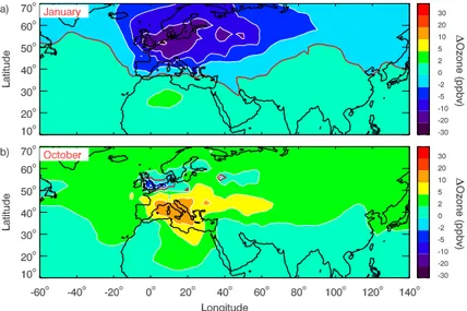
Figure 6 shows the monthly-averaged ozone perturbation near the surface for Jan-uary and October 2001. In contrast to summer (Fig. 4), the perturbation in winter is negative over all of Europe, with the greatest negative perturbations (<−10 ppbv) 10

co-located with high NO_x emissions over northwest Europe; this occurs because the

titration of ozone by NO is more important than the photochemical production of ozone at this time of year. In fact, the ozone perturbation is negative (<−1 ppbv) over much

of the Northern Hemisphere (>40◦_{N) because of European emissions. In this sense,}

Europe exports “negative ozone” to the mid and high latitudes during winter. However,

15

northern Africa and the Near East show a modest (∼1 ppbv) positive perturbation. The

changeover from a negative to a positive ozone perturbation, the zero perturbation line, is found in the Mediterranean Sea in January (Fig. 6a). The zero perturbation line moves northward into southern Europe through spring and vice-versa in autumn (Fig. 6b). In these transition times, the perturbation is negative typically over England

20

and the Benelux region, regions with the highest NOxemissions.

Additional violations of the European health standard for ozone due to European pollution typically occur from March through October in the Mediterranean Sea region. Figure 7a shows the number of additional violations in July, when there are at least 10 additional violations over Egypt, including the heavily populated Nile River valley, much

25

(14)

ACPD

8, 1913–1950, 2008

on ozone

B. N. Duncan et al.

Title Page

Tables Figures

◭ ◮

Back Close

Full Screen / Esc

EGU

figure, additional violations are found in much of the Middle East as well, including the Arabian peninsula, Iraq, Iran, Pakistan, and even as far downwind as China.

Our estimate of the number of additional violations may be high as our model surface ozone tends to be biased high in Europe in summer as discussed above; however there are few, if any, observations of surface ozone in northern Africa and the Near East with

5

which to evaluate our model bias in these regions.

5 Impact of European emissions on human mortality

In this section, we estimate the impacts of ozone associated with European emis-sions, presented above, on premature human mortality. We follow the methods of West et al. (2006) in estimating the number of premature mortalities in the Northern

10

Hemisphere, due to ozone from European emissions. We do not estimate the effects

of changes in particulate matter concentrations on mortality, but note that particulate matter has been strongly related with mortality (Pope et al., 2002). An assessment of the total burden of European air pollutant emissions on premature human mortality would need to also include particulate matter. We also acknowledge the potential for

15

European emissions to impact quality of life (e.g., from increased illness) and the econ-omy (e.g., from an increased number of sick days of employees or reduced crop yield) though we do not estimate these impacts here.

The equation for the change in human mortalities (_∆Mort) due to a change in ozone

concentration (∆O3) used in the epidemiological studies and in this study is:

20

∆Mort=−y0

e−β∆O₃ −1

P op (3)

wherey0 is the baseline mortality rate for a given population,β is the mortality

coef-ficient determined by the epidemiological studies (the fraction of additional mortalities

per ppbv of ozone), andPop is the total population. We use theβ for 8-h daily

maxi-mum ozone determined by Bell et al. (2004), who use a large database of 95 cities in

25

the United States and a distributed lag method. We select thisβbecause it is not

(15)

ACPD

8, 1913–1950, 2008

on ozone

B. N. Duncan et al.

Title Page

Tables Figures

◭ ◮

Back Close

Full Screen / Esc

theβfrom recent meta-analyses (Bell et al., 2005; Ito et al., 2005; Levy et al., 2005)

would give∼30% more mortalities. While this value ofβwas determined in the United

States, similar results have been found in Europe (Gryparis et al., 2004) and in some of the relatively fewer studies conducted in less industrialized nations (Borja-Aburto et al., 1998; Kim et al., 2004; O’Neill et al., 2004).

5

The distribution of population is taken from the LandScan database (Oak Ridge, 2005) for the 2003 population, which is then mapped onto the grid used for atmospheric

modeling. Values ofy0are derived from the World Health Organization (2004) for the

total non-accident baseline mortality in each of fourteen world regions. Changes in mortality are calculated on each day and in each model grid cell using the change in

10

8-h ozone concentration between RUN1 and RUN2, using the appropriate population

andy0for each cell. We assume a low-concentration threshold of 25 ppbv, below which

changes in ozone are assumed to have no effect on human mortality.

Table 2 shows the changes in population-weighted annual average 8-h daily max-imum ozone concentrations and in premature mortality in several regions of the

15

Northern Hemisphere. Here we see that when removing European emissions, the population-weighted ozone decrease is actually greater in the Near East than in Eu-rope itself, with substantial decreases also in the Former Soviet Union and northern Africa (considering the portion of Africa in the Northern Hemisphere), in agreement

with Figs. 4 and 6. Note that the European region extends to 60◦_{E, which includes}

20

about 68% of the population of the Former Soviet Union. Therefore, RUN2 includes re-ductions in emissions for most of the industrialized regions of the Former Soviet Union, including all of Belarus and Ukraine and parts of Russia and Kazakhstan.

The premature ozone-related mortalities resulting from European emissions are shown in Fig. 8. This distribution of mortalities is the result of the spatial distribution

25

of the change in ozone, the population distribution, and the baseline mortality rates in

different regions. The figure shows that the greatest density of premature mortalities

(16)

ACPD

8, 1913–1950, 2008

on ozone

B. N. Duncan et al.

Title Page

Tables Figures

◭ ◮

Back Close

Full Screen / Esc

EGU

greater density of population than in Mediterranean Europe. Algeria also has a greater baseline mortality rate than Western Europe, while Egypt, Jordan, Israel and Lebanon have baseline mortality rates roughly equal to or less than those in Western Europe.

We estimate that the total burden of European emissions on ozone-related mortality in the Northern Hemisphere is about 51 000 premature mortalities per year (Table 2).

5

Of these, roughly 37% percent occur in the European source region itself, with the majority of the premature mortalities outside of this source region. This finding that Eu-ropean emissions actually cause more ozone-related mortalities outside of the source region is consistent with other recent findings using another global CTM (West et al.,

20081), and will be discussed further below. Roughly 21% of the mortalities are in

10

Africa, and 16% are in the Near East. Interestingly, there are also fairly large numbers of premature mortalities in South Asia, East Asia, and even in North America; while the change in ozone concentration is small in these regions, the numbers of people exposed are large. We find that European emissions decrease mortalities in some re-gions of England and Benelux, due to the increased titration of ozone by reaction with

15

fresh NO emissions.

Figure 9 shows that the greatest number of premature mortalities per million people in the population occurs in the regions bordering the Mediterranean Sea, where the change in ozone is the greatest. Among the regions in Table 2, the premature mor-talities per million people are greatest in Europe. In Fig. 9, some discontinuities are

20

seen at national boundaries; for example, Tunisia is markedly lower than the bordering Algeria. This occurs because the WHO (2004) defines baseline mortality rates in world regions, and Tunisia is in a WHO region that has a much lower baseline mortality rate than Algeria.

In general, the uncertainty in ozone-related mortality calculations, such as those

25

presented here, is fairly substantial (West et al., 2006; West et al., 2007). Here we are interested in particular in the percentage of total mortalities that occur outside

1

(17)

ACPD

8, 1913–1950, 2008

on ozone

B. N. Duncan et al.

Title Page

Tables Figures

◭ ◮

Back Close

Full Screen / Esc

of Europe, for which two sources of uncertainties are particularly important. First,

for lack of better information, we apply a β determined in United States throughout

the Northern Hemisphere. Populations in other world regions may have a different

susceptibility to ozone mortality as the general causes of death often differ substantially between regions, and in particular, between the industrialized and developing nations.

5

To attempt to account for these differences in causes of death, we limit the calculation

to only cardiovascular and respiratory (CR) mortalities, using theβdetermined by Bell

et al. (2004) for CR mortalities and the appropriate baseline mortality rates for CR mortalities. In doing so, we find that European emissions cause about 33 500 ozone-related CR mortalities annually, and that the majority of these (57%) are still outside of

10

the European source region.

Second, some epidemiological studies of ozone-related mortality, all in temperate regions, have found different results in summer than in winter (Gryparis et al., 2004; Ito et al., 2005; Levy et al., 2005), while other studies have found no significant di_fference

between seasons (Bell et al., 2004). Since other regions affected by European

emis-15

sions do not experience the same seasonal difference in ozone as the United States

and Europe, we used a low-concentration threshold of 25 ppbv in the above results, rather than distinguishing between seasons. We test the sensitivity of our results to this approach first by increasing the low-concentration threshold, which will exclude more winter days in Europe. Raising the threshold to 40 ppbv gives 37 700 premature

all-20

cause mortalities in the Northern Hemisphere, with 66% of these mortalities outside of Europe. Second, we exclude the winter months, focusing on the period of April through October and using a 25 ppbv threshold. Doing so, we find that that European emissions cause 44 800 premature mortalities in the Northern Hemisphere, with a slight majority (51%) of these mortalities in Europe itself. If ozone truly does not affect mortality in the

25

(18)

ACPD

8, 1913–1950, 2008

on ozone

B. N. Duncan et al.

Title Page

Tables Figures

◭ ◮

Back Close

Full Screen / Esc

EGU

6 Conclusions

In this study, we used the GMI CTM to assess the impact of European pollution on surface ozone in 2001. The ability of the model to reproduce observations reasonably well, despite its limitations discussed in Sect. 3.1, lends confidence in its use as a tool to study the impact of European pollution on air quality in northern Africa and the Near

5

East.

We show that European pollution regularly and significantly elevates surface ozone

above the European health standard (i.e., 8-h average of 120µg/m3 or ∼60 ppbv) in

northern Africa and the Near East, especially in summer when prevailing winds favor transport from Europe to these photochemically productive regions. In July, European

10

pollution elevates average surface ozone in northern Africa by 10–20 ppbv and by 5– 10 ppbv in the Near East. For perspective, European pollution elevates surface ozone by typically 10–30 ppbv over southern Europe and 10–20 ppbv over northern Europe.

We estimate that European pollution causes 20–30 and 10–25 additional violations of the European health standard in July in northern Africa and the Near East,

respec-15

tively. That is, more than half of the days in July exceed the health standard because of the long-range transport of European pollution. High levels of ozone, above the thresh-old for the health standard and 2.5–3 times higher than background, were measured in the boundary layer over the Mediterranean Sea in summer 2001 during the MINOS field campaign and attributed to European pollution (Lelieveld et al., 2002). Annually,

20

there are between 50 and 150 additional violations of the health standard in northern Africa and the Near East because of European pollution. European emissions elevate ozone throughout most of the year in these regions (e.g., by 2–10 ppbv in October), though minimally in winter. In fact, European emissions actually decrease ozone over

most of Europe and latitudes higher than 40◦_{N in winter, due to titration of ozone by}

25

(19)

ACPD

8, 1913–1950, 2008

on ozone

B. N. Duncan et al.

Title Page

Tables Figures

◭ ◮

Back Close

Full Screen / Esc

While the contribution of European pollution to ozone in northern Africa and the Near East is high (Fig. 4c), it becomes even more important when one considers that the ozone in these regions in our simulation without European pollution (i.e., RUN2) is closer to the health standard than in Europe itself (Fig. 4b); this occurs as the pho-tochemical environment in northern Africa and the Near East is more conducive (e.g.,

5

ample sunlight) to ozone production as compared to the typical environment in Europe. Consequently, the exported European pollution has a large impact on surface ozone in northern Africa and the Near East, especially since the long-range transport of ozone and its precursors from Europe occurs near the surface.

We show that European pollution has a significant impact on human health outside

10

of Europe’s borders despite the uncertainty associated with this estimate of additional

deaths (e.g., the limited understanding of the effect of ozone on mortality outside the

United States and Europe) and the limitations of the model simulation as discussed in Sect. 3.1. We estimate that 50 000 additional deaths occur annually due to ozone produced from European pollution, with 19 000 of those deaths occurring in northern

15

Africa and the Near East and the majority of deaths attributed to European ozone occurring outside of Europe. About 9500 additional deaths also occur far downwind in

South and East Asia; while the contribution from European ozone is small (<5 ppbv in

July), large populations are exposed. While we focused on the year 2001, European pollution likely impacts air quality in northern Africa and the Near East in other years

20

as well, as southward flow from Europe at low altitudes typically occurs each year, especially in summer (Duncan and Bey, 2004).

Our results indicate that pollution control strategies within European countries, im-plemented to minimize local violations of the health standard for ozone, would also help to abate ozone pollution in countries in northern Africa and the Near East, with

25

benefits for public health in these regions. The Task Force on Hemispheric Transport of

Air Pollution (http://www.unece.org/env/tfhtap/) recently sponsored a CTM study to

(20)

ACPD

8, 1913–1950, 2008

on ozone

B. N. Duncan et al.

Title Page

Tables Figures

◭ ◮

Back Close

Full Screen / Esc

EGU

but not northern Africa and the Near East. Our results show that air quality in northern Africa and the Near East would benefit from an international approach to managing air quality.

Acknowledgements. We would like to thank the GMI science team for their efforts which has facilitated our research. The emissions database used in this manuscript was merged by J. Lo-5

gan and other researchers of Harvard University. This research was supported by NASA Grant MAP/04-0068-0040.

References

Anderson, H. R., Atkinson, R. W., Peacock, J. L., Marston, L., and Konstantinou, K.: Meta-analysis of time-series studies and panel studies of particulate matter (PM) and ozone (O₃), 10

World Health Organization, Geneva, 80 pp., 2004.

Auvray, M. and Bey, I.: Long-range transport to Europe: Seasonal variations and implications for the European ozone budget, J. Geophys. Res., 110, D11303, doi:10.1029/2004JD005503, 2005.

Bell, M. L., McDermott, A., Zeger, S. L., Samet, J. M., and Dominici, F.: Ozone and short-term 15

mortality in 95 US urban communities, 1987–2000, JAMA, 292(19), 2372–2378, 2004. Bell, M. L., Dominici, F., and Samet, J. M.: A meta-analysis of time-series studies of ozone

and mortality with comparison to the National Morbidity, Mortality, and Air Pollution Study, Epidemiology, 16(4), 436–445, 2005.

Bell, M. L., Peng, R. D., and Dominici, F.: The exposure-response curve for ozone and risk of 20

mortality and the adequacy of current ozone regulations, Environ. Health Perspect., 114(4), 532–536, 2006.

Berntsen, T. K., Karlsdottir, S., and Jaffe, D. A.: Influence of Asian emissions on the composition of air reaching the North Western United States, Geophys. Res. Lett., 26, 2171–2174, 1999. Bhartia, P. K., McPeters, R. D., Mateer, C. L., Flynn, L. E., and Wellemeyer, C.: Algorithm 25

for the estimation of vertical ozone profiles from the backscattered ultraviolet technique, J. Geophys. Res., 101, 18 793–18 806, 1996.

da Silva, A., Dee, D., Bloom, S., et al.: Documentation and validation of the Goddard Earth Observing System (GEOS) Data Assimilation System – Version 4, Technical Report Series on Global Modeling and Data Assimilation 104606, 187 pp., 2005.

(21)

ACPD

8, 1913–1950, 2008

on ozone

B. N. Duncan et al.

Title Page

Tables Figures

◭ ◮

Back Close

Full Screen / Esc

Interactive Discussion Borja-Aburto, V. H., Castillejos, M., Gold, D. R., Bierzwinski, S., and Loomis, D.: Mortality

and ambient fine particles in southwest Mexico City, 1993–1995, Environ. Health Perspect., 106(12), 849–855, 1998.

Challen, P. D., Hickish, D., and Bedford, J.: An investigation of some health hazards in an inert-gas tungsten-arc welding shop, Br. J. Ind. Med., 15, 276–282, 1958.

5

Chameides, W. L., Fehsenfeld, F., Rodgers, M.O., et al.: Ozone precursor relationships in the ambient atmosphere, J. Geophys. Res., 97, 6037–6055, 1992.

Chen, G., Huey, L. G., Trainer, M., et al.: An investigation of the chemistry of ship emission plumes during ITCT 2002, J. Geophys. Res., 110, D10S90, doi:10.1029/2004JD005236, 2005.

10

Chevalier, A., Gheusi, F., Delmas, R., et al. : Influence of altitude on ozone levels and variability in the lower troposphere : a ground-based study for western Europe over the period 2001– 2004, Atmos. Chem. Phys., 7, 4311–4326, 2007,

http://www.atmos-chem-phys.net/7/4311/2007/.

Chin, M., Ginoux, P., Kinne, S., Torres, O., Holben, B., Duncan, B., Martin, R., Logan, J., 15

Higurashi, A., and Nakajima. T.: Tropospheric aerosol optical thickness from the GOCART model and comparisons with satellite and sunphotometer measurements, J. Atmos. Sci., 59, 461–483, 2002.

Collins, W. J., Stevenson, D. S., Johnson, C. E., and Derwent, R. G.: The European regional ozone distribution and its links with the global scale for the years 1992 and 2015, Atmos. 20

Environ., 34, 255–267, 2000.

Davis, D. D., Grodzinsky, G., Kasibhatla, P., et al.: Impact of ship emissions on marine boundary layer NO_x and SO₂ distributions over the Pacific basin, Geophys. Res. Lett., 28, 235–238, 2001.

de Laat, A. T. J., Aben, I., and Roelofs, G. J.: A model perspective on total tropospheric O₃ 25

column variability and implications for satellite observations, J. Geophys. Res., 110, D13303, doi:10.1029/2004JD005264, 2005.

Duncan, B. N. and Bey, I.: A Modeling Study of the Export Pathways of Pollution from Eu-rope: Seasonal and Interannual Variations (1987–1997): J. Geophys. Res., 109, D08301, doi:10.1029/2003JD004079, 2004.

30

Duncan, B. N., Strahan, S. E., and Yoshida, Y.: Model study of the cross-tropopause transport of biomass burning pollution, Atmos. Chem. Phys., 7, 3713–3736, 2007,

(22)

ACPD

8, 1913–1950, 2008

on ozone

B. N. Duncan et al.

Title Page

Tables Figures

◭ ◮

Back Close

Full Screen / Esc

EGU

Eyring, V., Kohler, H. W., van Aardenne, J., and Lauer, A.: Emissions from international ship-ping: 1. The last 50 years, J. Geophys. Res., 110, D17305, doi:10.1029/2004JD005619, 2005.

Fiore, A. M., Jacob, D. J., Field, B. D., Streets, D. G., Fernandes, S. D., and Jang, C.: Linking ozone pollution and climate change: The case for controlling methane, Geophys. Res. Lett., 5

29(19), 1919, doi:10.1029/2002GL015601, 2002a.

Fiore, A. M., Jacob, D. J., Mathur, R., and Martin, R. V.: Application of empirical orthogonal functions to evaluate ozone simulations with regional and global models, J. Geophys. Res., 108, 4431, doi:10.1029/2002JD003151, 2003.

Fiore, A. M., Horowitz, L. W., Purves, D. W., et al.: Evaluating the contribution of changes 10

in isoprene emissions to surface ozone trends over the eastern United States, J. Geophys. Res., 110, D12303, doi:10.1029/2004JD005485, 2005.

Gryparis, A., Forsberg, B., Katsouyanni, K., et al.: Acute effects of ozone on mortality from the “Air pollution and health: A European approach” project, Am. J. Respir. Crit. Care Med., 170(10), 1080–1087, 2004.

15

Guenther, A., Karl, T., Harley, P., Wiedinmyer, C., Palmer, P. I., and Geron, C.: Estimates of global terrestrial isoprene emissions using MEGAN (Model of Emissions of Gases and Aerosols from Nature), Atmos. Chem. Phys., 6, 3181–3210, 2006,

Hallet, W.: Effect of ozone and cigarette smoke on lung function, Arch. Environ. Health, 10, 20

295–302, 1965.

Ito, K., De Leon, S. F., and Lippman, M.: Associations between ozone and daily mortality, Epidemiology, 16(4), 446–457, 2005.

Jacob, D. J., Logan, J. A., Yevich, R. M., et al.: Simulation of summertime ozone over North America, J. Geophys. Res. 98, 14 797–14 816, 1993a.

25

Jacob, D. J., Logan, J. A., Gardner, G. M., et al.: Factors regulating ozone over the United Sates and its export to the global atmosphere, J. Geophys. Res., 98, 14 817–14 826, 1993b. Jacob, D. J., Logan, J. A., and Murti, P. P.: Effect of rising Asian emissions on surface ozone in

the United States, Geophys. Res. Lett., 26, 2175–2178, 1999.

Jacobson, M. Z.: Computation of global photochemistry with SMVGEAR II, Atmos. Environ., 30

29, 2541–2546, 1995.

(23)

ACPD

8, 1913–1950, 2008

on ozone

B. N. Duncan et al.

Title Page

Tables Figures

◭ ◮

Back Close

Full Screen / Esc

Interactive Discussion Kasibhatla, P., Levy II, H., Moxim, W. J., et al.: Do emissions from ships have a significant

impact on concentrations of nitrogen oxides in the marine boundary layer?, Geophys. Res. Lett., 27, 2229–2232, 2000.

Kim, S. Y., JongTae, L., Lee, J. T., et al.: Determining the threshold effect of ozone on daily mortality: an analysis of ozone and mortality in Seoul, Korea, 1995-1999, Environ. Res., 5

94(2), 113–119, 2004.

Kleinfield, M., Giel, C., and Tabershaw, I.: Health hazards associated with inert gas shield metal arc welding, Arch. Ind. Health, 15, 27–31, 1957.

Kuhns, H., Green, M., and Etyemezian, V.: Big Bend Regional Aerosol and Visibility Observa-tional (BRAVO) Study Emissions Inventory, Desert Research Institute Report, 2003.

10

Lelieveld, J., Berresheim, H., Borrmann, S., et al.: Global air pollution crossroads over the Mediterranean, Science, 298, 794–799, 2002.

Levy, J. I., Carrothers, T. J., Tuomisto, J. T., Hammitt, J., and Evans, J. S.: Assessing the public health benefits of reduced ozone concentrations, Environ. Health Perspect., 109(12), 1215–1226, 2001.

15

Levy, J. I., Chemerynski, S. M., and Sarnat, J. A.: Ozone exposure and mortality: an empiric Bayes metaregression analysis, Epidemiology, 16(4), 458–468. 2005.

Li, Q., Jacob, D., Bey, I., et al.: Transatlantic transport of pollution and its effect on surface ozone in Europe and North America, J. Geophys. Res., 107(D13), 4166, doi:10.1029/2001JD001422, 2002.

20

Liang, J., and Jacobson, M. Z.: Effects of subgrid segregation on ozone production efficiency in a chemical model, Atmos. Environ., 34, 2975–2982, 2000.

Lin, X., Trainer, M., and Liu, S. C.: On the nonlinearity of the tropospheric ozone production, J. Geophys. Res., 93, 15 879–15 888, 1988.

Liu, S. C., Trainer, M., Fehsenfeld, F. C., et al.: Ozone production in the rural troposphere and 25

implications for regional and global ozone distributions, J. Geophys. Res., 92, 4194–4207, 1987.

Liu, H., Jacob, D. J., Bey, I., and Yantosca, R. M.: Constraints from210Pb and 7Be on wet deposition and transport in a global three-dimensional chemical tracer model driven by as-similated meteorological fields, J. Geophys. Res., 106, 12 109–12 128, 2001.

30

(24)

ACPD

8, 1913–1950, 2008

on ozone

B. N. Duncan et al.

Title Page

Tables Figures

◭ ◮

Back Close

Full Screen / Esc

EGU

McClinden, C. A., Olsen, S. C., Hannegan, B., Wild, O., Prather, M. J., and Sundet, J.: Strato-spheric ozone in 3-D models: A simple chemistry and the cross-tropopause flux, J. Geophys. Res., 105, 14 653–14 665, 2000.

Monks, P. S.: A review of the observations and origins of the spring ozone maximum, Atmos. Environ., 34, 3545–3561, 2000.

5

Murazaki, K. and Hess, P.: How does climate change contribute to surface ozone change over the United States?, J. Geophys. Res., 111, D05301, doi:10.1029/2005JD005873, 2006. Oak Ridge National Laboratory, Land Scan 2003,http://www.ornl.gov/sci/landscan/index.html,

accessed January 2005.

Olivier, J. G. J., Berdowski, J. J. M., Peters, J. A. H. W., Bakker, J., Visschedijk, A. J. H., 10

and Bloos, J.-P. J.: Applications of EDGAR. Including a description of EDGAR 3.0: reference database with trend data for 1970-1995. RIVM, Bilthoven. RIVM report no. 773301 001/ NOP report no. 410200 051, 2001.

Olsen, S. C., McLinden, C. A., and Prather, M. J.: Stratospheric N₂O-NO_y system: Testing un-certainties in a three-dimensional framework, J. Geophys. Res., 106, 28 771–28 784, 2001. 15

O’Neill, M. S., Loomis, D., and Borja-Aburto, V. H.: Ozone, area social conditions, and mortality in Mexico City, Environ. Res., 94(3), 234–242, 2004.

Park, R. J., Pickering, K. E., Allen, D. J., Stenchikov, G. L., and Fox-Rabinovitz, M. S.: Global simulation of tropospheric ozone using the University of Maryland Chemical Transport Model (UMD-CTM): 2. Regional transport and chemistry over the central United States using a 20

stretched grid, J. Geosphys. Res., 109, D09303, doi:10.1029/2003JD004269, 2004.

Piccot, S., Watson, J., and Jones, J.: A global inventory of volatile organic compound emissions from anthropogenic sources, J. Geophys. Res., 97, 9897–9912, 1992.

Pope, C. A., Burnett, R. T., Thun, M. J., et al.: Lung cancer, cardiopulmonary mortality, and long-term exposure to fine particulate air pollution, JAMA, 287(9), 1132–1141, 2002. 25

Prather, M., Gauss, M., Berntsen, T., et al.: Fresh air in the 21st century?, Geophys. Res. Lett., 30, 1100, doi:10.1029/2002GL016285, 2003.

Reiter, R., Sladkovic, R., and Kanter, H.-J.: Concentration of trace gases in the lower tropo-sphere, simultaneously recorded at neighboring mountain stations, Meteorol. Atmos. Phys., 37, 27–47, 1987.

30

(25)

ACPD

8, 1913–1950, 2008

on ozone

B. N. Duncan et al.

Title Page

Tables Figures

◭ ◮

Back Close

Full Screen / Esc

Interactive Discussion Sander, S. P., Friedl, R. R., Ravishankara, A. R., et al.: Chemical Kinetic and Photochemical

Data for Use in Atmospheric Studies, Evaluation Number 15, NASA Jet Propulsion Labora-tory, JPL Publication 06-2, 523 pp., 2006.

Schoeberl, M. R., Duncan, B. N., Douglass, A. R., Waters, J., Livesey, N., Read, W., and Filipiak, M.: The carbon monoxide tape recorder, Geophys. Res. Lett., 33, L12811, 5

doi:10.1029/2006GL026178, 2006.

Sillman, S., Logan, J. A., and Wofsy, S. C.: A regional scale model for ozone in the United States with subgrid representation of urban and power plant plumes, J. Geophys. Res., 95, 5731–5748, 1990.

Song, C. H., Chen, G., Hanna, S. R., Crawford, J., and Davis, D. D.: Dispersion and chemical 10

evolution of ship plumes in the marine boundary layer: Investigation of O₃/NO_y/HO_x chem-istry, J. Geophys. Res., 108, 4143, doi:10.1029/2002JD002216, 2003.

Stockinger, H.: Ozone toxicology: A review of research and industrial experience, Arch. Envi-ron. Health, 10, 719–731, 1965.

Stohl, A., Eckhardt, S., Forster, C., James, P., and Spichtinger, N.: On the pathways 15

and timescales of intercontinental air pollution transport, J. Geophys. Res., 107, 4684, doi:10.1029/2001JD001396, 2002.

Stohl, A., Forster, C., Eckhardt, S., Spichtinger, N., Huntrieser, H., Heland, J., Schlager, H., Wilhelm, S., Arnold, F., and Cooper, O.: A backward modeling study of intercon-tinental pollution transport using aircraft measurements, J. Geophys. Res., 108, 4370, 20

doi:10.1029/2002JD002862, 2003.

Strahan, S. E., Duncan, B. N., and Hoor, P.: Observationally derived transport diagnostics for the lowermost stratosphere and their application to the GMI chemistry and transport model, Atmos. Chem. and Phys., 7, 2435–2445, 2007.

Streets, D. G., Bond, T. C., Carmichael, G. R., et al.: An inventory of gaseous and 25

primary aerosol emissions in Asia in the year 2000, J. Geophys. Res., 108, 8809, doi:10.1029/2002JD003093, 2003.

Streets, D. G., Zhang, Q., Wang, L., He, K., Hao, J., Wu, Y., Tang, Y., and Carmichael G. R.: Revisiting China’s CO emissions after TRACE-P: Synthesis of inventories, atmospheric modeling, and observations, J. Geophys. Res, 111, D14306, doi:10.1029/2006JD007118, 30

2006.

(26)

ACPD

8, 1913–1950, 2008

on ozone

B. N. Duncan et al.

Title Page

Tables Figures

◭ ◮

Back Close

Full Screen / Esc

EGU

Traub, M., Fischer, H., de Reus, M., et al.: Chemical characteristics assigned to trajectory clusters during the MINOS campaign, Atmos. Chem. Phys., 3, 459–468, 2003,

Trickl, T.,Cooper, O. R., Eisele, H., James, P., M ¨ucke, R., and Stohl, A.: Intercontinental trans-port and its influences on the ozone concentrations over central Europe: Three case studies, 5

J. Geophys. Res., 108, doi:10.1029/2002JD002735, 2003.

Versteng, V., Breivik, K., Adams, M., et al.: Inventory Review 2005, Emission Data reported to LRTAP Convention and NEC Directive, Initial review of HMs and POPs, Technical report MSC-W 1/2005, ISSN 0804-2446, 2005.

von Glasow, R., Lawrence, M. G., Sander, R., and Crutzen, P. J.: Modeling the chemical effects 10

of ship exhaust in the cloud-free marine boundary layer, Atmos. Chem. Phys., 3, 233–250, 2003,http://www.atmos-chem-phys.net/3/233/2003/.

West, J. J., Fiore, A. M., Horowitz, L. W., and Mauzerall, D. L.: Global health benefits of miti-gating ozone pollution with methane emission controls, Proc. Natl. Acad. Sci. USA, 103(11), 3988–3993, 2006.

15

West, J. J., Szopa, S., and Hauglustaine, D. A.: Human mortality effects of future concentrations of tropospheric ozone, Comptes Rendus de l’Acadme des Sciences – Geoscience/, 339, 775–783, doi:10.1016/j.crte.2007.08.005, 2007.

Wild, O., Pochanart, P., and Akimoto, H.: Trans-Eurasian transport of ozone and its precursors, J. Geophys. Res., 109, D11302, doi:10.1029/2003JD004501, 2004.

20

Wild, O. and Prather, M.: Global tropospheric ozone modeling: Quantifying errors due to grid resolution, J. Geophys. Res., 111, D11305, doi:10.1029/2005JD006605, 2006.

World Health Organization: The World Health Report 2004: Changing History, World Health Organization, Geneva, 169 pp., 2004.

Wunderli, S. and Gehrig, R.: Surface ozone in rural, urban and alpine regions of Switzerland, 25

Atmos. Environ. Part A, 24, 2641–2646, 1990.

Young, W., Shaw, D., and Bates., D.: Effects of low concentrations of ozone on pulmonary function in man, J. Appl. Physiol., 19, 765–768, 1964.

Ziemke, J. R., Chandra, S., Duncan, B. N., Froidevaux, L., Bhartia, P. K., Levelt, P. F., and Waters, J. W.: Tropospheric ozone determined from Aura OMI and MLS: Evaluation of mea-30

(27)

ACPD

8, 1913–1950, 2008

on ozone

B. N. Duncan et al.

Title Page

Tables Figures

◭ ◮

Back Close

Full Screen / Esc

Table 1. Statistical Comparison of the Model’s Daily Maximum 8-h Averages with those of

EMEP Ozone Observationsafor June, July and August 2001.

Station ID Lat deg Lon deg Altm ∆b% R2c _Violationsd

(28)

ACPD

8, 1913–1950, 2008

on ozone

B. N. Duncan et al.

Title Page Abstract Introduction Conclusions References Tables Figures ◭ ◮ ◭ ◮ Back Close

Full Screen / Esc

EGU

Table 1.Continued.

Station ID Lat deg Lon deg Altm ∆b_% _R2c _Violationsd

FI09 59.8 21.4 7 9.8 0.72 0 2 FI37 62.6 24.2 180 1.1 0.37 0 0 FR08 48.5 7.1 775 −7.2 0.81 38 22 FR09 49.9 4.6 390 11.1 0.78 16 27 FR10 47.3 4.1 620 28.7 0.73 7 20 FR12 43.0 −1.1 1300 −6.5 0.68 30 2 FR13 43.4 0.1 236 20.2 0.61 7 3 FR14 47.2 6.5 746 24.7 0.59 14 22 GB02 55.3 −3.2 243 37.1 0.59 0 6 GB06 54.4 −7.9 126 21.8 0.35 0 0 GB13 50.6 −3.7 119 32.3 0.47 4 14 GB14 54.3 −0.8 267 21.9 0.60 4 10 GB36 51.6 −1.3 137 −1.5 0.71 3 4 GB38 50.8 0.2 120 14.5 0.61 11 18 GB43 51.2 −4.7 160 22.5 0.65 1 10 GB45 52.3 −0.3 5 −3.1 0.80 10 6 HU02 47.0 19.6 125 0.4 0.69 31 7 IT01 42.1 12.6 48 1.9 0.59 64 61 IT04 45.8 8.6 209 −13.2 0.40 39 8 LT15 55.4 21.1 5 23.6 0.50 1 24 NL09 53.3 6.3 1 41.1 0.57 2 16 NL10 51.5 5.9 28 3.5 0.65 13 10 NO01 58.4 8.3 190 37.5 0.20 0 9 NO15 65.8 13.9 439 −8.7 0.48 0 0 NO39 62.8 8.9 210 20.2 0.08 0 0 NO41 61.3 11.8 440 −2.7 0.31 0 0 PL02 51.8 22.0 180 5.4 0.18 6 0 PL03 50.7 15.7 1603 10.8 0.50 25 28 PL04 54.8 17.5 2 6.1 0.41 3 4 PL05 54.2 22.1 157 5.7 0.25 1 0 RU18 54.9 37.8 150 21.3 0.23 0 0 SE02 57.4 11.9 10 3.5 0.50 4 5 SE11 56.0 13.2 175 11.7 0.51 3 12 SE12 58.8 17.4 20 20.7 0.75 1 7 SI08 45.6 14.9 520 25.7 0.29 35 59 AVGe _9.9 _0.54 _15.5 _14.9

MEDf 9.5 0.57 11.0 10.0

a

Station descriptions are atwww.nilu.no/projects/CCC/sitedescriptions/index.html.

b

The bias (%) is the mean of (model-observed)/observation for the time period; the number of daily observations coincident with the model output are between 86 and 92.

c

R is the linear correlation coe_fficient between the model and observations.

d

Number of violations of the 8-h European ozone standard (_∼60 ppbv).

e

Average of 67 stations.

f

(29)

ACPD

8, 1913–1950, 2008

on ozone

B. N. Duncan et al.

Title Page

Tables Figures

◭ ◮

Back Close

Full Screen / Esc

Table 2. Decreases in ozone (the population-weighted annual average 8-h daily maximum)

when European emissions are removed, including premature mortalities per year, in each of eight Northern Hemisphere regions.

Premature Premature Regiona Pop. ∆O₃ mortalities mortalities (millions) (ppbv) (/yr) (/million/yr)

Europe 688.9 6.0 18 800 27.3

Northern Africa 626.4 4.1 10 700 17.1

Near/Middle Eastb 408.6 7.0 8400 20.5

Former Soviet Unionc 98.7 4.5 1700 17.7

South Asiad 1267.1 0.8 3800 3.0

East Asiae 1518.5 1.4 5800 3.8

Southeast Asiaf 361.9 0.4 300 1.0

America 578.7 0.9 1400 2.4

Total Northern Hemisphere 5548.8 2.5 51 000 9.2

a

Regions are defined in only the Northern Hemisphere.

b

Turkey, Cyprus, Israel, Jordan, Syria, Lebanon, countries on the Arabian Peninsula, Iraq, Iran, Afghanistan, and Pakistan.

c

East of 60◦_{E; west of 60}◦_{E and north of 44}◦_{N is considered part of the “Europe” region.}

d

India, Bangladesh, Sri Lanka, Nepal, and Bhutan.

e

Japan, Mongolia, China, Taiwan, North Korea, and South Korea.

f

(30)

ACPD

8, 1913–1950, 2008

on ozone

B. N. Duncan et al.

Title Page

Tables Figures

◭ ◮

Back Close

Full Screen / Esc

EGU

Fig. 1.Monthly-average ozone (13:00–17:00 LT; ppbv) at selected EMEP stations for 2001 for

(31)

ACPD

8, 1913–1950, 2008

on ozone

B. N. Duncan et al.

Title Page

Tables Figures

◭ ◮

Back Close

Full Screen / Esc

Fig. 2.Observed (black) and modeled (red) maximum 8-h average ozone (ppbv) for June, July,

(32)

ACPD

8, 1913–1950, 2008

on ozone

B. N. Duncan et al.

Title Page

Tables Figures

◭ ◮

Back Close

Full Screen / Esc

EGU

Fig. 3.The(a)model (2001) and(b)observed (2005) TCO (DU) for July.(c)The portion of the

(33)

ACPD

8, 1913–1950, 2008

on ozone

B. N. Duncan et al.

Title Page

Tables Figures

◭ ◮

Back Close

Full Screen / Esc

Fig. 4.Monthly-average surface ozone (1–24 h; ppbv) for July 2001 for the(a)RUN1 (i.e., base

(34)

ACPD

8, 1913–1950, 2008

on ozone

B. N. Duncan et al.

Title Page

Tables Figures

◭ ◮

Back Close

Full Screen / Esc

EGU Fig. 5. Vertical cross-section at 15◦_{E of the di}