Flexural behaviour of selected plants under static load

(1)

HESSD

7, 1459–1483, 2010

Flexural behaviour of selected plants under

static load

F. J. Sutili et al.

Title Page

Abstract Introduction

Conclusions References

Tables Figures

◭ ◮

Back Close

Full Screen / Esc

Printer-friendly Version

Interactive Discussion Hydrol. Earth Syst. Sci. Discuss., 7, 1459–1483, 2010

www.hydrol-earth-syst-sci-discuss.net/7/1459/2010/ © Author(s) 2010. This work is distributed under the Creative Commons Attribution 3.0 License.

Hydrology and Earth System Sciences Discussions

This discussion paper is/has been under review for the journal Hydrology and Earth System Sciences (HESS). Please refer to the corresponding final paper in HESS if available.

Flexural behaviour of selected plants

under static load

F. J. Sutili1, L. Denardi2, M. A. Durlo2, H. P. Rauch3, and C. Weissteiner3

1

The Commission for Development Studies, OeAD Gmbh, Vienna, Austria 2

Federal University of Santa Maria, Rio Grande do Sul, Campus Universit ário – Centro de Ci ências Rurais (Agricultural Center) – Post-Graduation Program in Forest Engineering, Pr édio 44 – 2oPiso CEP, 97105-900, Santa Maria-RS, Brazil

3

Institute of Soil Bioengineering and Landscape Construction, University of Natural Resources and Applied Life Sciences, Vienna, Peter Jordan-Str. 82, 1190, Vienna – Austria

Received: 20 January 2010 – Accepted: 30 January 2010 – Published: 24 February 2010

Correspondence to: H. P. Rauch (hp.rauch@boku.ac.at)

(2)

HESSD

7, 1459–1483, 2010

static load

F. J. Sutili et al.

Title Page

Tables Figures

◭ ◮

Back Close

Full Screen / Esc

Interactive Discussion

Abstract

One of the principal purposes of soil bioengineering is the application of vegetation layers from a civil engineering point of view. Living plants are used to reinforce slopes and to control erosion. For a standardised implementation, it is essential to quantify the effectiveness and to assess technical parameters for such bioengineering systems.

5

The objective of this study is to investigate the flexibility of stems and branches of dif-ferent riparian species of the area of Southern Brazil suitable for soil bioengineering (Phyllanthus sellowianus M üll. Arg., Sebastiania schottiana (M üll. Arg.) M üll. Arg.,

Salix humboldtiana Willd., andSalix×rubens Schrank). Fifty specimens (green stem

samples) were collected in the surroundings of Santa Maria, state of Rio Grande do

10

Sul, Brazil, and subjected to static bending tests. Their overall deformation behaviour (elastic and plastic) is of crucial importance for bioengineering systems. Thus, addi-tional to the state of the art of material parameters, a new parameter is introduced: the “angle of flexibility”. This parameter describes the elastic and plastic deformation behaviour of a plant under load in a more engineering practival experience. The results

15

show that the species ofPhyllanthus sellowianusis the most flexible species, followed bySebastiania schottiana,Salix humboldtianaandSalix×rubens.

1 Introduction

In the centre of the federal state of Rio Grande do Sul (Brazil) many farmers have problems from the erosion of river banks which in turn causes erosion of agriculturally

20

useful land. Consequently farmers are interested in sustainably stabilised river banks to protect their farmland which provides a more stable economic foundation. Stabilised riverbanks also guarantee that artificially constructed irrigation channels work properly. These channels can be managed efficiently when riparian areas show more or less stable morphological conditions. Additional public awareness has been gained for

ero-25

sion control for riverbanks and agricultural land when natural hazards cause damage

(3)

HESSD

7, 1459–1483, 2010

static load

F. J. Sutili et al.

Title Page

Tables Figures

◭ ◮

Back Close

Full Screen / Esc

Interactive Discussion to infrastructure facilities. The techniques of soil bioengineering may provide suitable

instruments to counter these problems (Schiechtl et al., 1994).

Drawing on the results from a previous study which focused on the vegetative re-production potential of suitable plants for soil bioengineering (Sutili et al., 2007), the next step involved quantifying the biomechanical behaviour of plants under specific

5

load. The quantification of these processes is a crucial point establishing standards and function related dimensioning of soil bioengineering techniques from an engineer-ing point of view. The application of plants in river engineerengineer-ing project is based on a proven knowledge about the interaction of plants and flow.

The hydraulic interaction of flow with plants depends not only on geometrical

proper-10

ties (e.g. stem and branch diameter, length and leaf density), but also on the dynamic response of plants under flood conditions (stem/branch/leaf bending and reduction of plant height; e.g. Fathi-Moghadam and Kouwen, 1997; Oplatka, 1998; Gerstgraser, 2000; Meixner et al., 2004; Rauch, 2005, Rhigetti and Armanini, 2002; Musley and Cruise, 2006; McBride et al., 2007). Mechanical properties such as flexural stiffness,

15

modulus of elasticity and plastic deformation are indicators to assess the impact of plants on hydraulic conditions. The modulus of elasticity, the proportional limit, as well as the deformation and stress up to the point of rupture are shown in a typical stress×deformation diagram (Fig. 1). The first part of the diagram is a straight line that

determines the modulus of elasticity and the limit of elastic behaviour. From this point

20

the deformation becomes plastic and continues up to the point of rupture (B in Fig. 1) in a non-proportional way.

The objective of this study is to investigate the flexibility of stems and branches of different riparian species suitable for soil bioengineering (Phyllanthus sellowianusM ¨ull. Arg.,Sebastiania schottianaM ¨ull. Arg., Salix humboldtiana Willd., andSalix×rubens 25

(4)

HESSD

7, 1459–1483, 2010

static load

F. J. Sutili et al.

Title Page

Tables Figures

◭ ◮

Back Close

Full Screen / Esc

2 Plant material and methods

Although riparian vegetation is exposed to dynamic stress during flood events, static bending tests are useful to identify the bending behaviour of different plant species. The results have to be considered as a comparison between di_fferent species.

The specimens were collected along rivers in the surroundings of the municipality of

5

Santa Maria. Phyllantus sellowianus is part of the spurge family (Euphorbiaceae) and grows up to a height of 2–3 m. It is a widely ramified bush with slender and bendable branches. Sebastiana schottianais also a shrub with a maximum height of 3–4 m. It is provided with strong branches wich are higly bendable.Salix×rubensoriginally comes

from Europe and is a hybrid betweenSalix albaandSalix fragilis. The plant grows very

10

fast and reaches heights up to 16 m. Finally,Salix humboltianais a tree which reaches a height up to 20 m and a stem diameter of about 90 cm. All of the tested species are known to be well adapted to the riverine environment conditions along rivers.

Fifty static bending tests of each species were carried out, using samples of different diameters. The minimum diameter was defined at 10 mm and the bending device

lim-15

ited the maximum diameter. ForPhyllanthus sellowianus and Sebastiania schottiana,

no samples that exceeded a diameter of 50 mm for the former and 60 mm for the latter were found in the area under study. The specimens were tested with their bark imme-diately after harvesting. The setup of the bending tests is based on the DIN standard (DIN 52186) for 3 point loading tests. The specimens must have a minimum length

20

of 14 times the diameter at point loading. The bending device of the laboratory is de-signed for samples with a maximum length of one meter, which means the maximum diameter is limited to 70 mm. The lengths of the samples were adapted according to the length-diameter ratio proposed in the DIN 52186.

The testing equipment automatically recorded the parameters loadF [N],

displace-25

mentf [mm] and timet [s]. Based on the collected data sets (F [N], f [mm] andt [s]) as well as on the measured diameters d [mm] of the specimens at the point of load and on the distance between the points of support l [mm], it was possible to determine

(5)

HESSD

7, 1459–1483, 2010

static load

F. J. Sutili et al.

Title Page

Tables Figures

◭ ◮

Back Close

Full Screen / Esc

Interactive Discussion the following parameters:

– proportional limit load,Felast[N]

– breaking load (maximum),F_B [N]

– modulus of elasticity (MOE),E [N/mm2] – proportional limit stress,σelast [N/mm

2

]

5

– breaking stress (modulus of rupture, MOR),σB[N/mm2]

– elastic deformation,ǫelast [−]

– plastic deformation,ǫplast [−]

– breaking deformation (maximum),ǫB[−]

– inertial moment,I [mm4]

10

– maximum momentM [N/mm] – maximum resistanceW [mm3]

After each bending test, a 100 mm long sample was taken to determine the following parameters:

– moisture content in wood,u[%]

15

– basic apparent specific weight of the wood,ρ[g/cm3] – thickness of bark,tc[mm]

– percentage of bark, %c [%]

(6)

HESSD

7, 1459–1483, 2010

static load

F. J. Sutili et al.

Title Page

Tables Figures

◭ ◮

Back Close

Full Screen / Esc

2.1 Calculating the parameters

The breaking load F_B and proportional limit load Felast were directly taken from the

load×displacement diagram. The modulus of elasticityE(also called Young’s modulus)

is used to characterise the elastic behaviour of the stems and branches. This mechan-ical parameter expresses the ratio between the stress and the deformation under load,

5

i.e., how much force is required for a given unit of reversible deformation. Accordingly, the modulus of elasticity can be taken as an indicator for rigidity rather than flexibil-ity. The modulus of elasticityE [N/mm2] for specimens with a circular cross-section, supported on two points and exposed to a load at a central point, is calculated as:

E= Felast·l 3

48·Felast·I ,

10

where:

Felast proportional limit load [N],

l distance between the support points [mm],

felastdisplacement up to proportional limit [mm], Iinertial moment [mm4].

15

The inertial moment (I) [mm4] for a circular section was calculated as:

I=π·d 4

64 ,

whered [mm] is the diameter of the specimen measured at the point of load appli-cation.

Replacingl in the formula above, the equation changes to:

20

E= Felast·l 3

3·felast·π·d 4 4

.

(7)

HESSD

7, 1459–1483, 2010

static load

F. J. Sutili et al.

Title Page

Tables Figures

◭ ◮

Back Close

Full Screen / Esc

Interactive Discussion The deformation ǫ [−] is a dimensionless variable that can be calculated at the

pro-portional limitǫelast and at the rupture limitǫB, thus also including the range of plastic

deformation:

ǫ=f·12·d

l2 ,

where:

5

f displacement (at the elastic or at the rupture limit) [mm],

d diameter of the specimen at the point of load application [mm],

l distance between the support points [mm].

The formulae used for the analysis of E and ǫ are based on the assumption that

10

the segment has a constant diameter and shear stress is neglected. Tree stems are generally tapered, in our case the diameter of the specimens were approximately con-stant, therefore the tapering e_ffect is negligible. For wood shear stress is conventionally neglected ifl /d >14. Usually bending resistance of wood is determined with a 4-point bending test. The results of the used 3-point test are influenced by shear strains which

15

are neglected. However, the used formulae are to be considered as an approximation but results are highly appropriate to compare the species between each other.

The breaking stress σ_B [N/mm2] (modulus of rupture, MOR) for specimens with a circular cross-section was obtained by:

σ_B=M W =

FB·l /2

π·d3

32

=16·FB·l π·d3

,

20

where:

Mmaximum moment [Nmm],

W maximum resistance [mm3],

FB breaking load [N],

l distance between the points of support [mm],

(8)

HESSD

7, 1459–1483, 2010

static load

F. J. Sutili et al.

Title Page

Tables Figures

◭ ◮

Back Close

Full Screen / Esc

d diameter of the specimen at the point of load application [mm].

The stress up to the proportional limitσelast [N/mm 2

] can be obtained by the previous formula, replacing the breaking loadF_B [N] by the load up to the proportional limitFelast

[N] or by “Hooke’s Law,” which determines:

5

σelast=E·ǫelast,

where:

E modulus of elasticity [N/mm2],

ǫelast deformation up to proportional limit [−]. 10

The moisture contentu[%] of the wood was calculated as:

u=mu_m−mo o

·100

where:

muwet mass of the specimen [g],

m_o dry mass of the specimen [g]. and the basic apparent specific weight of the wood

15

ρ[g/cm3] as:

ρ=mo V

where:

m_odry mass of the wood [g],

V volume of wood [cm3].

20

The thickness of the bark was measured using a digital calliper, and the percentage of the bark %c [%] was determined as the ratio between the area of the bark ring and the total cross-section of the specimen:

%c=At−Ao A_t ·100,

25

(9)

HESSD

7, 1459–1483, 2010

static load

F. J. Sutili et al.

Title Page

Tables Figures

◭ ◮

Back Close

Full Screen / Esc

Interactive Discussion where:

Attotal area (wood+bark) [cm 2

],

Ao area without bark [cm2].

After preparation and staining of histological sections a microscope was used to

5

determine the age of the samples.

A new value, the angle of flexibility, was introduced. It describes the whole deforma-tion process of plants under load:

– angle of flexibility at proportional limit,αelast[◦],

– angle of flexibility at the point of rupture,αB[◦].

10

At the original non-inflected position (dashed horizontal line in Fig. 2), the bending point divides the specimen into two equal parts with an angle of zero to the horizontal and 180◦ _{between the two. With the values of} _l _and _f _{at the proportional limit and at the} breaking limit, it is possible to calculate the angle of flexibility (α), respectively αelast

andαB (Fig. 2).

15

α=2·atan2·f

l

where:

l distance between the points of support [mm],

f displacement (at the proportional limit or at the point of rupture, respectively) [mm].

3 Results and discussion

20

3.1 Basic apparent specific weight, moisture content and bark

(10)

HESSD

7, 1459–1483, 2010

static load

F. J. Sutili et al.

Title Page

Tables Figures

◭ ◮

Back Close

Full Screen / Esc

Interactive Discussion andSalix×rubensshow some proportional relationship (tendency) between increasing

diameter and the basic apparent specific weight and a slight inverse relationship to the moisture content of the wood. No such relationship tendency can be found for

Phyllanthus sellowianus. The values of basic apparent specific weight of the wood ofPhyllanthus sellowianus were relatively high compared to the other three species,

5

probably because of its slower growth and the higher average age of the specimens of this species.

As expected, the thickness of the bark strongly correlates with the diameters and maintains a relatively constant percentage up to the highest diameters of this study. The two species that have a lower average bark thickness – Phyllanthus sellowianus

10

andSebastiania schottiana– consequently show a more discreet increase in the bark thickness with the increase in diameter. Salix humboldtiana represents the thickest bark from 5 mm up to 7 mm for stem diameters between 60 and 70 mm. Br ¨uchert et al. (2003) finds that the higher initial bark/wood ratio and its decline with the develop-ment of the branch may collaborate toward the initial variations regarding the modulus

15

of elasticity (E). For bending tests all samples were tested with the bark on.

3.2 Modulus of elasticity

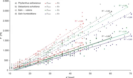
Figure 3 indicates the force (F) needed to reach the proportional limit (solid line) or to reach the point of rupture (dashed line), for different diameters.

For the same diameter, Phyllanthus sellowianus is the most resistant species and

20

Salix humboldtiana the most fragile. This means that for Phyllanthus sellowianus a higher amount of load is necessary to reach the point of elastic limit and the point of rupture, respectively.

Table 1 shows the results of calculating the modulus of elasticity for the di_fferent species arranged by diameter classes. The coefficient of variation [%] is shown in

25

brackets alongside the average. The last column contains the coefficient of determina-tion between the modulus of elasticity and the stem and branch diameter.

(11)

HESSD

7, 1459–1483, 2010

static load

F. J. Sutili et al.

Title Page

Tables Figures

◭ ◮

Back Close

Full Screen / Esc

Interactive Discussion Vollsinger et al. (2000) for green stems and branches of five European species (Alnus

glutinosa (L.) Gaertn., Fraxinus excelsior L., Salix alba L., Salix caprea L. and Acer pseudoplatanus L.). The authors obtained values between 6.900 and 10.200 N/mm2 for the different species (with diameters of 40 to 100 mm). Based on parameter (E), the tested southern Brazilian species are visibly less rigid.

5

The modulus of elasticity (Table 1) declines with the increase in diameter. However, this suggestion of an inverse correlation between the modulus of elasticity and the stem diameter must be considered with caution due to the high coe_fficients of variation CV

and the low coefficients of determination. Vollsinger et al. (2000) found similar results. Br ¨uchert et al. (2003) conducted tests onAlnus glutinosa(L.) Gaertn. andAlnus viridis

10

(Chaix) DC. of an age from 1 to 24 years and found a slight increase in the modulus of elasticity up to the fifth year. In older samples the modulus of elasticity remained relatively constant. Niklas (1992) notes that young cell walls are ductile, while older cells walls tend to be much more elastic and resilient.

3.3 Proportional and rupture limit

15

Deformation is irreversible for inert materials once the proportional limit has been passed. For plants this limit becomes less important, because they remain alive and have the ability to regenerate, even when the proportional limit is greatly exceeded. This phenomenon can be observed in riparian vegetation right after flooding. When plants have not returned to their original position after the water level has dropped,

20

this means that their proportional limit has been exceeded. Yet, the plants still have the biological capacity to recover gradually and adapt their habit to the new local en-vironmental conditions. Even after exceeding the rupture limit, plants with vegetative reproduction potential are able to regenerate.

Thus the limit of rupture is an important parameter, apart from the modulus of

elas-25

(12)

HESSD

7, 1459–1483, 2010

static load

F. J. Sutili et al.

Title Page

Tables Figures

◭ ◮

Back Close

Full Screen / Esc

Interactive Discussion the deformation behaviour at the rupture point between the different species is

sub-ject to greater variation. The two Euphorbiaceae (Sebastiania schottiana and espe-cially Phyllanthus sellowianus) are capable of resisting large deformation and larger stresses prior to the point of rupture. Salix humboldtianasupports slightly less stress thanSalix×rubens. Salix humboldtiana, however, shows a higher deformation in com-5

parison toSalix×rubens.

3.4 Angle of flexibility

The dimensionless deformation ǫ can be understood as an expression of how the material behaves under load. The angle of flexibility up to the proportional limit (αelast)

or up to point of rupture (α_B) is another way to demonstrate this deformation.

10

The angle of flexibility at the proportional limit and the diameter do not correlate significantly. Theαelast area in Fig. 5 limits the range where potentially any species at

any diameter reaches the proportional limit angle. Figure 5 also shows the relationship betweenα_Band the stem and branch diameter. A parameter that can be easily used in practice, the angle of flexibility at the point of rupture textitαBrepresents the maximum

15

angle to which a stem or branch of a particular species and diameter can be bent at the point of rupture. The results have to be considered as a base to compare the bending ability of the tested species.

The diagram shows that Phyllanthus sellowianus forms a larger angle of flexibility at the point of rupture than the other species. For example, while a 20 mm branch of

20

Phyllanthus sellowianuscan form a 45◦ _{angle of flexibility before breaking, a branch of}

Salix×rubensof the same diameter only reaches 24◦before breaking.

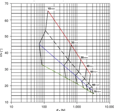
Figure 6 summarises the angle of flexibility at the rupture point (α_B) with the breaking load (FB) required for the four species across the distribution of the stem and branch

diameters. The nomogram shown in Fig. 6 cannot be used to reproduce the values at

25

the proportional limit due to the lack of a relationship between the angle of flexibility and the diameter at this limit (Fig. 5).

(13)

HESSD

7, 1459–1483, 2010

static load

F. J. Sutili et al.

Title Page

Tables Figures

◭ ◮

Back Close

Full Screen / Esc

Interactive Discussion diameter, while its angle of flexibility at rupture point decreases. Thus, a branch of

Phyllanthus sellowianusmeasuring 20 mm in diameter must be stressed up to a load of 670 N to hit the point of rupture and forms a 45◦ _{angle of flexibility. A branch of}

Sebastiania schottianaof the same diameter, with a load of 550 N, breaks at 36◦_._Salix

humboldtianaforms a smaller angle of flexibility (32◦_{) and requires a load of 400 N to}

5

reach the breaking point. For the same diameter, Salix×rubens – despite having an

angle of flexibility at rupture point that is even lower than the previous species – needs a higher load (460 N) thanSalix humboldtianato reach a maximum 25◦_{angle of flexibility} at rupture point.

As demonstrated in Fig. 6, the flexibility gradually declines with the increase in

diam-10

eter and age.Phyllanthus sellowianus is the species that supports the greatest stress and can be bent to higher angles of flexibility at the breaking point. Moreover, its growth rate is the lowest of all species investigated. The following diagram (Fig. 7) shows the relationship between the age of the stems and branches and their diameter.

The relationships shown in Fig. 7 can not be generalised due to different local

en-15

vironmental conditions, but can be taken as reference values for the growth rate. In a following step the growth rate (diameter and age) is related to the angle of flexibility at rupture point (αB) and shown in the nomogram in Fig. 8.

The relationship between age and stem diameter can be seen directly on thex- and

y-axes, respectively. The angle of flexibility at the point of rupture is characterised

20

by means of the marked areas. For example, in order to know the diameter of each species in the fourth year of age, trace a straight line parallel to the y-axis at the age of 4 years. At the point where this line crosses the straight line that defines the relations forPhyllanthus sellowianus, you will get a diameter of 16 mm and an angle of flexibility at the point of rupture of 50◦_{. At the same age,}_{Sebastiania schottiana}_{has a diameter}

25

of 23 mm and a 33◦_{angle of flexibility at the point of rupture (interpolated between the} lines of 30◦_{and 35}◦_). _Salix

×rubens at 4 years shows a diameter of 32 mm and bends

(14)

HESSD

7, 1459–1483, 2010

static load

F. J. Sutili et al.

Title Page

Tables Figures

◭ ◮

Back Close

Full Screen / Esc

Interactive Discussion be applied starting from any diameter (d), age (Y) or angle of flexibility (α_B), for each

species. For the species investigated, Fig. 9 provides useful information for planning and managing soil bioengineering work in this region.

4 Conclusions and final remarks

The modulus of elasticity (E, Young’s modulus) does not satisfactorily explain the

flex-5

ibility of live branches for the assessment of soil bioengineering structures. The angle of flexibility up to the point of rupture (α) and the applied load proved to be more ap-propriate to characterise the stem flexibility of different species.

Using this parameter and the maximum breaking load (F_B), the bending properties of the plants can be determined. Stem flexibility is a better criterion to identify a plant’s

10

suitability to stabilise fluvial slopes. All the results must take into account the age of the plants. Based on the parametersα_B,F_B andY, it can be affirmed that plants of a smaller (younger) diameter are more flexible, regardless of species. The results show that the flexibility of the stems and branches diminishes over time but not equally or proportionally for each of the species studied.

15

Considering that large plants can cause instability on fluvial slopes (overload, lever e_ffect), there are su_fficient arguments to justify interventions such as pruning or even coppicing individuals when flexibility is lost.

It was proven thatPhyllanthus sellowianusand Sebastiania schottianaare very ap-propriate for the protection of fluvial slopes according to the criteria of stem flexibility,

20

resistance to rupture (stem breakage), growth rate and plant size. Riparian forest stands ofSalix humboldtiana and Salix×rubens need more frequent maintenance in

order to preserve branch flexibility. According to the literature, any of the four species studied can excellently withstand and respond to the pruning of branches and coppic-ing of trunks.

25

Bending tests and the newly introduced “angle of flexibility” (αB) parameter serve as

parameters to compare the species. In actual practice plants are stressed and bent

(15)

HESSD

7, 1459–1483, 2010

static load

F. J. Sutili et al.

Title Page

Tables Figures

◭ ◮

Back Close

Full Screen / Esc

Interactive Discussion in a way which is different from the bending in the laboratory and that needs further

research work. In nature the stresses on plants during high floods act dynamically and therefore the plants’ response is quite different from the static load test at the laboratory. Furthermore, the influence of the bark and the anatomical characteristics of the wood can be helpful to clarify additional biomechanical characteristics of the

5

riparian vegetation.

Acknowledgements. Work funded by the Commission for Development Studies at the OeAD Gmbh.

References

Br ¨uchert, F., Gallenm ¨uller, F., Bogenrieder, A., and Speck, T.: Stem mechanics, functional

10

anatomy and ecology ofAlnus viridisandAlnus glutinosa, Berlin, Feddes Repertorium, 114, 3–4, 181–197, 2003

DIN 52186: Pr üfung von Holz – Biegeversuch, Deutsches Institut f ür Normung, Berlin, 1978. Dittrich, A.: Wechselwirkung Morphologie/Str ömung naturnaher Fließgew ässer,

Habilitationss-chrift, TU-Karlsruhe, 208, ISSN 0176-5078, 1998.

15

Fathi-Moghadam, M. and Kouwen, N.: Nonrigid, nonsubmerged, vegetative roughness on floodplains, J. Hydr. Engrg., 123(1), 51–57, 1997.

Florineth, F.: Pflanzen statt Beton, Handbuch zur Ingenieurbiologie und Vegetationstechnik, Patzer Verlag Berlin, Hannover, ISBN 3-87617-107-5, 282 pp., 2004.

Gerstgraser, C.: Ingenieurbiologische Bauweisen an Fliessgew ¨assern. Grundlagen zu Bau,

20

Belastbarkeiten und Wirkungsweisen, Band 52, Dissertation, Univ. f ¨ur Bodenkultur, Wien, 2000.

Li, R.-M. and Shen, H. W.: Effect of tall vegetations on flow and sediment, J. Hydr. Eng. Div.-ASCE, 106(6), 1085–110, 1973.

Meixner, H.: Grunds ¨atze zum Management von Ufervegetation, Ingenieurbiologie,

Mitteilungs-25

blatt f ¨ur die Mitglieder des Vereins f ¨ur Ingenieurbiologie, Nr.2/2004, 14–18, ISSN 1422-008, 2004.

(16)

HESSD

7, 1459–1483, 2010

static load

F. J. Sutili et al.

Title Page

Tables Figures

◭ ◮

Back Close

Full Screen / Esc

Interactive Discussion Musleh, F. A. and Cruise, J. F.: Functional relationships of resistance in wide flood plains with

rigid unsubmerged vegetation, J. Hydr. Eng., 132(2), February 2006, 163–171, 2006. McBride, M., Hession, W. C., Rizzo, D. M., and Thompson, D. M.: The influence of riparian

vegetation on near-bank turbulence: A flume experiment, Earth Surf. Proc. Land., 32(13), 2020–2037, November 2007.

5

Niklas, K. J.: Plant Biomechanics – An engineering approach to plant form and function, Univ. of Chicago, Press Chicago and London, 580 pp., 1992.

Nuding, A.: Fließwiderstandsverhalten in Gerinnen mit Ufergeb ¨usch. Wasserbau – Mitteilungen des Instituts f ¨ur Wasserbau, konstruktiver Wasserbau und Wasserwirtschaft, TH Darmstadt, no. 35, 1991.

10

Oplatka, M.: Stabilit ät von Weidenverbauungen an Flussufern, Mitteilung 156, Versuchsanstalt f ür Wasserbau, Hydrologie und Glaziologie, ETH-Z ürich, 1998.

Pasche, E.: Turbulenzmechanismen in naturnahen Fliessgew ässern und die M öglichkeiten ihrer mathematischen Erfassung, Mitteilungen Inst. f ür Wasserbau und Wasserwirtschaft, No. 52, RWTH Aachen, 243 pp., 1984.

15

Pasche, E. and Rouve, G.: Overbank flow with vegetatively roughened flood plains, J. Hydraul Eng.-Asce., 111(9), 1262–1278, 1985.

Petryk, S. and Bosmaijian, G. B.: Analysis of flow through vegetation, Journal of the Hydraulic Division, ASCE, 101(7), 871–884, 1975.

Rauch, H. P.: Hydraulischer Einfluss von Geh ¨olzstrukturen am Beispiel der

ingenieurbiologis-20

chen Versuchsstrecke am Wienfluss, Dissertation an der Universit ¨at f ¨ur Bodenkultur Wien, 222 pp., 2005.

Rhigetti, M. and Armanini, A.: Flow resistance in open channel flows with sparsely distributed bushes, J. Hydrol., 269 pp., 55–64, 2002.

Schiechtl, H., Stern, R., et al.: Handbuch f ¨ur naturnahen Erdbau, Eine Anleitung f ¨ur

ingenieu-25

biologische Bauweisen, ¨Osterreichischer Agrarverlag, Wien, 160 pp., 1994.

Sutili, F. J., Rauch H. P., Durlo M. A., and Florineth, F: Investigations on the selection of plants for soil bioengineering measures in South Brazil, European Geoscience Union Assembly, 19 April 2007, Vienna, Poster, 2007.

Vollsinger, S., Doppler, F., and Florineth, F.: Ermittlung des Stabilit ¨atsverhaltes von

Ufer-30

geh ölzen in Zusammenhang mit Erosionsprozessen an Wildb ächen, Uni. f ür Bokenkultur, Wien, Studie in Auftrag des Bundesministeriums f ür Land- u. Forstwirtschaft, 107 pp., 2000.

(17)

HESSD

7, 1459–1483, 2010

static load

F. J. Sutili et al.

Title Page

Tables Figures

◭ ◮

Back Close

Full Screen / Esc

Interactive Discussion Table 1.Average values of the modulus of elasticity [N/mm2] for the different diameter classes

of each species. Coefficient of variation is shown in brackets ().

Modulus of elasticity [N/mm2] per diameter class

Species 10–20 mm 20–30 mm 30–40 mm 40–50 mm 50–60 mm 60–70 mm R2

Phyllanthus sellowianus 4.513 (20) 3.793 (31) 3.329 (25) 3.028 (27) − − 0.27

Sebastiania schottiana 4.615 (26) 3.930 (29) 4.104 (31) 3.485 (12) 3.114 (18) − 0.14

Salix×rubens 4.940 (35) 4.562 (29) 4.296 (25) 3.555 (34) 3.625 (21) 3.031 (11) 0.19

(18)

HESSD

7, 1459–1483, 2010

static load

F. J. Sutili et al.

Title Page

Tables Figures

◭ ◮

Back Close

Full Screen / Esc

×

E

B

σ

elast limit of proportionality

ε

elast

ε

B

σ

B

maximum load

Elastic zone

Plastic zone

×

Fig. 1.Typical stress×deformation diagram.

(19)

HESSD

7, 1459–1483, 2010

static load

F. J. Sutili et al.

Title Page

Tables Figures

◭ ◮

Back Close

Full Screen / Esc

α α

α α α

⋅ ⋅ = α

of rupture, respectively) [mm].

l

f

α

Fig. 2: Bent specimen, indicating the variables used in calculating the angle of flexibility (α).

×

(20)

HESSD

7, 1459–1483, 2010

static load

F. J. Sutili et al.

Title Page

Tables Figures

◭ ◮

Back Close

Full Screen / Esc

limit and the point of rupture respectively.

R2_{= 0,94}

d R2_{= 0,96}

c

R2_{= 0,96}

R2_{= 0,93}

0 500 1.000 1.500 2.000 2.500 3.000 3.500

10 20 30 40 50 60 70

d

F

[N]

d) Salix humboldtiana Felast FB c) Salix rubens× Felast FB b) Sebastiania schottiana Felast FB a) Phyllanthus sellowianus Felast FB

a

b

R2_{= 0,84}

R2_{= 0,89}

c

R2_{= 0,91}

d R2_{= 0,93}

Fig. 3. Relationship between diameter (d) and load (F). Solid line: Felast at the proportional limit; dashed line:F_Bat the point of rupture.

(21)

HESSD

7, 1459–1483, 2010

static load

F. J. Sutili et al.

Title Page

Tables Figures

◭ ◮

Back Close

Full Screen / Esc

[N/mm²]

ε

[-]

0 20 60 80 100

40

0 0,02 0,04 0,06 0,08 0,10 0,12 0,14

Phyllanthus sellowianus (a)

Sebastiania schottiana (b)

Salix rubens (c)

Salix humboldtiana (d)

a

b

c d

×

є

α α

α

Fig. 4.Deformation and stress at proportional limit (solid line) and at rupture limit (dashed line) for the four species.

(22)

HESSD

7, 1459–1483, 2010

static load

F. J. Sutili et al.

Title Page Abstract Introduction Conclusions References Tables Figures ◭ ◮ ◭ ◮ Back Close

Full Screen / Esc

Printer-friendly Version Interactive Discussion a d c b 0 5 10 15 20 25 30 35 40 45 50 55 60 65 70

10 20 30 40 50 60 70

d[mm] a B [° ] aelast

Salix humboldtiana(d) 0,64

Salixxrubens(c) 0,32

Phyllanthus sellowianus (a) 0,64

Sebastiana schottiana(b) 0,48

R² a d c b 0 5 10 15 20 25 30 35 40 45 50 55 60 65 70

10 20 30 40 50 60 70

d[mm] a B [° ] aelast

R²

α

Fig. 5.Relationship between the diameter (d) and the angle of flexibility at the point of rupture (α_B). The band at the bottom of the graph shows the area of distribution of the angles of flexibility at the proportional limit (α_elast).

(23)

HESSD

7, 1459–1483, 2010

static load

F. J. Sutili et al.

Title Page

Tables Figures

◭ ◮

Back Close

Full Screen / Esc

×

α

between the angle of flexibility and the diameter at this limit (Figure 5).

10mm

20mm

30mm

40mm

50mm

60mm

70mm

Phyllanthus sellowianus Sebastiania schottiana Salix humboldtiana

Salix rubens

100

10 1.000 10.000

20 30 40 50 60 70

10

FB [N]

B

[°

]

Fig. 6: Regression of α (angle of flexibility at the point of rupture) against log F _(breaking

×

Fig. 6. Regression ofα_B (angle of flexibility at the point of rupture) against log F_B (breaking load) for the four species, within the studied diameter classes.

(24)

HESSD

7, 1459–1483, 2010

static load

F. J. Sutili et al.

Title Page

Tables Figures

◭ ◮

Back Close

Full Screen / Esc

10 20 30 40 50 60 70

d[mm] 12

11

10 9 8

7 6 5

4 3 2

1 0

Y

[yea

rs]

Sebastiania schottiana (b) 0,83 Y=0,13d+1,04

Salix rubens (c) 0,58 Y=0,12d+0,15

Salix humboldtiana (d) 0,79 Y=0,09d+0,47 Phyllanthus sellowianus (a) 0,82 Y=0,24d+0,24

Species R² Model

a

b

c

d

Fig. 7: Relationship between the diameter (d_{) and the age (}Y_{) of stems and branches.}

α

Fig. 7.Relationship between the diameter (d) and the age (Y) of stems and branches.

(25)

HESSD

7, 1459–1483, 2010

static load

F. J. Sutili et al.

Title Page

Tables Figures

◭ ◮

Back Close

Full Screen / Esc

α

Phyllanthus sellowianus

Sebastiania schottiana

Salix humboldtiana

Salix rubens

0 20 30 40 50 60 70

10

Y [years]

d

[mm

]

1 2 3 4 5 6 7 8 9 10 11 12 13 14

15° 20°

25°

30° 20°

25°

30°

35°

40°

45°

50° 55° 60° 15°

interpretation example

α