A transfer function for the prediction of gas hydrate inventories in marine sediments

(1)

BGD

7, 1057–1099, 2010

Prediction of gas hydrate inventories

M. Marquardt et al.

Title Page

Abstract Introduction

Conclusions References

Tables Figures

◭ ◮

Back Close

Full Screen / Esc

Printer-friendly Version

Interactive Discussion

Biogeosciences Discuss., 7, 1057–1099, 2010 www.biogeosciences-discuss.net/7/1057/2010/ © Author(s) 2010. This work is distributed under the Creative Commons Attribution 3.0 License.

Biogeosciences Discussions

This discussion paper is/has been under review for the journal Biogeosciences (BG). Please refer to the corresponding final paper in BG if available.

A transfer function for the prediction of

gas hydrate inventories in marine

sediments

M. Marquardt, C. Hensen, E. Pi ˜nero, K. Wallmann, and M. Haeckel

Leibniz-Institut f ¨ur Meereswissenschaften, IFM-GEOMAR, Kiel, Germany

Received: 21 January 2010 – Accepted: 26 January 2010 – Published: 12 February 2010 Correspondence to: M. Marquardt ([email protected])

(2)

BGD

7, 1057–1099, 2010

M. Marquardt et al.

Title Page

Tables Figures

◭ ◮

Back Close

Full Screen / Esc

Abstract

A simple prognostic tool for gas hydrate (GH) quantification in marine sediments is presented based on a diagenetic transport-reaction model approach. One of the most crucial factors for the application of diagenetic models is the accurate formulation of mi-crobial degradation rates of particulate organic carbon (POC) and the coupled biogenic 5

CH₄formation. Wallmann et al. (2006) suggested a kinetic formulation considering the

ageing effects of POC and accumulation of reaction products (CH₄, CO₂) in the pore

water. This model is applied to data sets of several ODP sites in order to test its general validity. Based on a thorough parameter analysis considering a wide range of

environ-mental conditions, the POC accumulation rate (POCar in g/cm2/yr) and the thickness

10

of the gas hydrate stability zone (GHSZ in m) were identified as the most important and independent controls for biogenic GH formation. Hence, depth-integrated GH

invento-ries in marine sediments (GHI in g of CH₄ per cm2 seafloor area) can be estimated

as:

GHI₌a·POCar·GHSZb·exp(−GHSZc/POCar/d)+e

15

witha=0.00214, b=1.234, c=−3.339, d=0.3148, e=−10.265.

Several tests indicate that the transfer function gives a realistic approximation of the minimum potential GH inventory of low gas flux (LGF) systems. The overall advantage of the presented function is its simplicity compared to complex numerical models: only two easily accessible parameters are needed.

20

1 Introduction

(3)

BGD

7, 1057–1099, 2010

M. Marquardt et al.

Title Page

Tables Figures

◭ ◮

Back Close

Full Screen / Esc

loop (e.g. Dickens et al., 1995; Kennett et al., 2003; Milkov, 2004). (ii) The dissociation of GH creates overpressures in marine sediments that may trigger slope failure events (Xu and Germanovich, 2006). These mass wasting events may in turn damage cables, pipelines and further facilities for oil and gas production installed on the seabed. (iii) Natural gas bound in GH could become a profitable energy source because of contin-5

uously decreasing amounts of conventional fossil fuel resources. Pilot studies aiming at the exploitation of submarine GH are currently carried out in a number of countries (e.g. Japan, India, China, Norway, Germany). Among standard techniques to disso-ciate GH (i.e. pressure reduction, thermal simulation, and thermodynamic inhibitor

in-jection; Moridis et al., 2004; Sloan and Koh, 2007), a promising new approach of CO₂

10

exchange for CH₄ is currently investigated (Ersland et al., 2009; Zhou et al., 2008).

An improved estimate of mass and distribution of GH stored in marine sediments is a fundamental prerequisite to address these questions.

In general two di_fferent main types of marine GH occurrences are distinguished: high

gas flux systems (HGF) and low gas flux systems (LGF) (Milkov, 2005). HGF are de-15

fined by GH amounts with local concentrations from 5 to up to 100 vol.%. Kastner et al. (2008b) estimated GH concentrations in pore space saturation of up to 67 vol.% for the continental margin of India. Even higher concentrations of 90 vol.% are reported for Nankai by Uchida et al. (2004). Such high concentrations are the result of upward migrating fluids and gases from greater sediment depth which are often enriched in 20

thermogenic CH₄(Torres et al., 2004; Liu and Flemmings, 2007). From an economical

perspective, these are the most interesting areas for future GH-exploitation programs. In contrast, LGF seem to represent the main reservoirs for GH on a global scale. They encompass by far the largest area of active and passive continental margins with aver-age concentrations of about 2 vol.% (Milkov, 2005). Generally, the GH in LGF consists 25

mostly of biogenic CH₄which is produced within and below the GHSZ. Because of the

(4)

BGD

7, 1057–1099, 2010

M. Marquardt et al.

Title Page

Tables Figures

◭ ◮

Back Close

Full Screen / Esc

Estimates of the GH inventory

Various geochemical and geophysical methods have been developed and applied to quantify GH-inventories on various scales. However the predictions made since the early 80’s vary extremely by several orders of magnitude (Fig. 1). The early estimate of

5.5×1021g of CH4 stored in the global GH inventory (Dobrynin et al., 1981) has been

5

continuously corrected downward to about 1.4×1017g of CH4 (Soloviev, 2002) at the

turn of the millennium. More recently, there is again a slightly upward trend based on

studies by Bu_ffett and Archer (2004), Milkov (2004) and Klauda and Sandler (2005). At

present, an inventory of about 4×1018g of CH4(3000 Gt C) seems to be the most likely

scenario. 10

Overall, the estimates of the global GH inventory hold discrepancies and inaccura-cies of up to five orders of magnitude (Fig. 1). To some extent the mismatch between

the different approaches can be explained by the fact that global estimates are based

on local or at least regional models, which are then assumed to be representative at the global scale. Such extrapolations depend on a number of more or less constrained 15

parameters which lead to a high level of uncertainty. Typical geophysical approaches to quantify sub-seafloor GH include seismic velocity analysis (e.g. Chand et al., 2004; Westbrook et al., 2008), marine controlled source electromagnetic methods (CSEM; e.g. Chave and Cox, 1982; Schwalenberg et al., 2005), in-situ resistivity measure-ments (e.g. Kvenvolden, 1988; Yuan et al., 1996; Hyndman et al., 1999), and infrared 20

thermal scanning of sediment cores (e.g. Ford et al., 2003). Estimates based on the geochemical analysis of pore water usually comprise the interpretation of negative

Cl−_{-anomalies as caused by freshwater release during GH dissociation (e.g. Hesse,}

2003; Haeckel et al., 2004), and complementary results from pressure core sampling (Heeschen et al., 2007).

25

In addition, a number of studies (e.g. Davie and Bu_ffett, 2003; Torres et al., 2004;

(5)

BGD

7, 1057–1099, 2010

M. Marquardt et al.

Title Page

Tables Figures

◭ ◮

Back Close

Full Screen / Esc

GH inventories. The main advantage of transport-reaction models is to constrain rates of GH formation by control parameters such as the particulate organic carbon (POC)

input, POC degradation, sedimentation rate, pore water diffusion and advection, heat

flow, etc., which can be calibrated against measured pore water and solid phase data. The input and degradation of POC are most critical in this regard as they are the driv-5

ing force for CH₄formation (Davie and Buffett, 2001). Several authors used first order

kinetic rate laws for modelling the degradation of POC (Davie and Buffett, 2001), based

on the assumption that the formation of CH₄ is directly proportional to the availability

of incoming POC. Although various approaches have been suggested to describe this process (e.g. Berner, 1980; Westrich and Berner, 1984; Middelburg, 1989), it is still 10

di_fficult to provide generally valid constraints on the parameterization of these specific

rate laws. Moreover, input and composition of organic matter are usually not constant over time (e.g. Berner, 2003), and thus, a generalisation of the POC input and degrada-tion rates may not be appropriate. In some recent models for assessing the global GH

inventory (e.g. Bu_ffett and Archer, 2004; Bhatnagar et al., 2007; Archer et al., 2008)

15

rate parameterisations were chosen in a way that a fixed percentage of the POC-flux

to the seafloor is converted into CH₄and GH. In the present study, we test the general

validity of a model that uses a second order rate law for POC degradation as suggested by Wallmann et al. (2006) using data from a number of ODP sites. Based on this, we conducted systematic numerical model runs covering a broad range of environmental 20

conditions and geological settings in order to derive a simplified transfer function for the prediction of potential GH inventories.

2 Validation of the numerical model

The transport-reaction model developed by Wallmann et al. (2006) is based on a one-dimensional, numerical approach implemented in Wolfram Mathematica. The model 25

considers steady state compaction of the sediment, di_ffusive and advective transport

(6)

nitro-BGD

7, 1057–1099, 2010

M. Marquardt et al.

Title Page

Tables Figures

◭ ◮

Back Close

Full Screen / Esc

gen (PON) via sulfate reduction and methanogenesis, anaerobic oxidation of methane

(AOM), as well as the formation of NH₄, dissolved inorganic carbon (DIC) and CH₄.

The model calculates the solubility of CH₄ in pore water, the stability, formation and

dissociation of GH as well as the stability, formation and dissolution of free CH₄ gas

(FG) in pore water. The general equations and parameterizations of the model are 5

given in the Appendix (Tables A1 and A2); a more detailed description is provided by Wallmann et al. (2006). Specifically, the model calculates the POC-degradation rate as a function of POC input. The rate and reactivity of POC decrease with depth due to age-dependent alteration and inhibition by the accumulation of degradation products

(i.e. DIC and CH₄) in the pore water:

10

R_POC= KC

C(CH₄)+C(DIC)+K_C·

0.16·(ageinit+agesed)−0.95

·C(POC), (1)

whereRPOCis the degradation rate,KCis the inhibition coefficient for POC degradation,

C(CH₄),C(DIC) andC(POC) are the concentrations of the dissolved and solid species.

The central term is an age-dependent term after Middelburg (1989) with age_init as the

initial age of the POC, and age_sed as the alteration time of POC since entering the

15

sediment column.

Specifically the value ofK_cis crucial for limiting POC degradation at higher

concen-trations of CH₄and DIC. Wallmann et al. (2006) could show that this value seems to be

fairly constant (30 to 40 mM) based on results from the Sea of Okhotsk and ODP Site 997 (Blake Ridge). Hence, the major purpose of applying the model to data from vari-20

ous ODP sites is to prove if a generalised parameterisation of POC kinetics is feasible to receive good fits to data from diverse geological environments. Therefore, the model was applied to data from ODP Site 1041 (Costa Rica), Sites 685 and 1230 (Peru), Site 1233 (Chile), Site 1014 (California), Site 995 (Blake Ridge), and Site 1084 (Namibia). GH were previously recovered and/or confirmed at ODP Sites 1041, 685, 1230 and 25

(7)

BGD

7, 1057–1099, 2010

M. Marquardt et al.

Title Page

Tables Figures

◭ ◮

Back Close

Full Screen / Esc

Kimura et al., 1997; Mix et al., 2003; Paull et al., 1996; Suess et al., 1988; Westbrook et al., 1994) and is summarised in Table 1. Overall, sedimentary strata between 200 and 800 mbsf were recovered from these sites. At Site 1041 the bottom of the stabil-ity zone (BSZ) is not reached within the sedimentary deposits. In general, the overall

POC concentrations are high (>0.5 wt.%) and the SO₄-penetration depth is low and

5

accompanied by a strong increase of sub-surface NH₄- and CH₄-levels.

Each of the standard models was run into steady state by fitting the model to

concentration-depth profiles of the dissolved species SO₄ and NH₄ and the solid

species POC and PON. Standard runs consider constant POC input over time as well

as sediment burial and molecular diffusion as the only transport processes (a-model

10

run runs). Additional runs with variable POC input (b-model runs) and fluid advection (c-model runs) were performed as specified below (Table 1) in order to comply with site-specific conditions.

All model results (including predicted GH volumes) and measured concentrations of

SO₄, NH₄, POC, and PON (if available) are shown in Figs. 2–7. The boundary

con-15

centrations used in this study are listed in Table A2 of the Appendix. For all models

the concentrations at the upper boundary of the dissolved species SO₄, CH₄and NH₄

have been prescribed to fixed values corresponding to standard seawater composi-tion (Dirichlet condicomposi-tions). At the lower boundary zero-gradient condicomposi-tions are chosen for the a- and b-models (Neumann conditions). For the c-models, which consider ad-20

vective fluid flow from below, the concentrations of the dissolved species have been

determined as Dirichlet conditions. Therefore, the SO₄- and NH₄-concentrations at

the lower boundary were set to zero and CH₄-concentration was taken from the

out-put of the respective a-model. The inout-put of POC at the upper boundary is given by a fixed concentration, which is modulated into a time-dependent function considering 25

variations in the POC input over time for the b-models:

POC(x=0)₌f(t) (2)

(8)

BGD

7, 1057–1099, 2010

M. Marquardt et al.

Title Page

Tables Figures

◭ ◮

Back Close

Full Screen / Esc

Pore water SO₄ and NH₄ are the most important parameters for fitting the model.

POC and PON usually show more natural variability, and hence are more di_fficult

to constrain. At the depth where CH₄-saturation with respect to methane hydrate is

reached (calculated after Tishchenko et al., 2005) GH starts to precipitate. Average GH concentrations without considering fluid flow are generally below 1% of the pore 5

volume (Figs. 2–7). These comparatively low concentrations are in agreement with

recent studies at locations which are not affected by intense fluid or gas flow (Milkov,

2005; Tr ´ehu et al., 2004).

2.1 Site-specific results

2.1.1 Costa Rica

10

Site 1041 is located at the active, erosive continental margin of Costa Rica at a water

depth of about 3300 m. Measured data at this location can be sufficiently represented

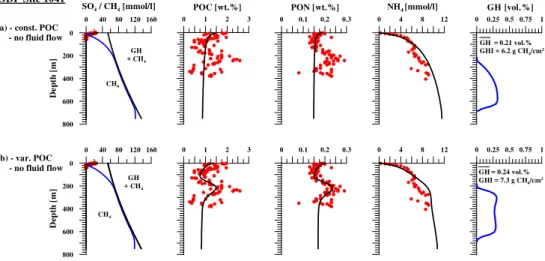
by the standard model (Fig. 2). However, POC and PON data indicate considerable variations in the input of organic material over time. In order to evaluate to which extent

such variations may affect GH inventories a second run was performed where the POC

15

input at the sediment surface was varied over time. The result is a better fit to POC

and PON data, which, however, only a_ffects estimated GH concentrations by about

20%. Slight deviations from the measured NH₄profile in both runs may be explained

by lateral advection of fluids (Hensen and Wallmann, 2005), which may explain local GH occurrences between 115 and 165 mbsf at this site (Kimura et al., 1997). However, 20

since this process is probably of minor importance and also very difficult to constrain,

it will not be further addressed in this study.

2.1.2 Peru

(9)

BGD

7, 1057–1099, 2010

M. Marquardt et al.

Title Page

Tables Figures

◭ ◮

Back Close

Full Screen / Esc

part of the accretionary wedge that forms due to subduction of the Nazca plate. At

Site 1230, SO₄ and NH₄ profiles are well reproduced by the standard model (Fig. 3).

An average of the measured POC concentrations was used as the POC input value in order to comply with the considerable scatter observed in the depth profile. The GH content is 0.64 vol.% on average and extends from about 60 to 260 mbsf, which excel-5

lently matches with the depth interval reported for GH findings (D’Hondt et al., 2003). However, the sedimentary sequence recovered at the nearby Site 685 is considerably

thicker (620 m) and indicates that NH₄ decreases with depth (Fig. 3). A model run

without fluid flow results in a NH₄-profile which is not supported by the data, but

re-veals GH concentrations purely based on in situ degradation rates (Fig. 3). Average 10

GH inventories in the no-flow scenarios are approximately the same at both locations, and hence give a good approximation of minimum GH inventories. Based on drilling

results (D’Hondt et al., 2003) and similar to findings offshore Costa Rica (Hensen and

Wallmann, 2005), upward advection of deep-seated NH₄-depleted fluids is a likely

ex-planation for the observed decrease in NH₄. In a second model run, we applied an

15

upward advection rate of 0.16 mm yr−1 _{and varied the model parameterisation}

accord-ingly in order to fit the model to the NH₄ data (Table 1). In agreement with previous

studies (Bu_ffett and Archer, 2004; Hensen and Wallmann, 2005) GH inventories in

this scenario increase significantly from 26 g of CH₄/cm2(a-model) to 66 g of CH₄/cm2

(c-model). 20

2.1.3 Southern Chile

Site 1233 is located in a small forearc basin on the upper continental margin (840 mbsf)

offshore Southern Chile, belonging to the southern end of the Nazca subduction

sys-tem. The area is characterised by very high sedimentation rates of about 100 cm/kyr. The standard model does not produce a good fit to the data and does not predict 25

any formation of GH (Fig. 4). The mismatch is obviously caused by changes in the

POC input over time and, considering the down-core decrease of NH₄, most likely

(10)

BGD

7, 1057–1099, 2010

M. Marquardt et al.

Title Page

Tables Figures

◭ ◮

Back Close

Full Screen / Esc

POC-data and the sedimentation rate), however, improved the fit to the data, but did not change the result with respect to GH accumulation. Additional consideration of fluid flow results in a good fit to the data (c-model in Fig. 4) and predicts the presence of

minor amounts of GH between 60 and 80 mbsf. All in all, the in situ production of CH₄

is most likely not su_fficient to produce GH at this site.

5

2.1.4 California

Site 1014 was drilled in the Tanner Basin, which belongs to the band of California Borderland basins and is characterised by high organic matter input and an extended oxygen minimum zone between 500 and 1500 m water depth. The standard model revealed a good fit to the measured data (Fig. 5). However, the scatter in the POC 10

input over time was not resolved in the a-run. An average input value of 5 wt.% of POC

produced an excellent fit to the measured NH₄ profile, and hence is obviously a good

approximation of the overall POC degradation. In spite of the high POC accumulation, GH are not reported for this site. Most likely this is due to the high geothermal gradient

of 58◦_{/km resulting in a thin GHSZ. The model predicts minor amounts of GH at the}

15

BSZ.

2.1.5 Blake Ridge

The Blake Ridge ODP Site 995, which was drilled into a large drift deposit located at the passive continental margin of the south-eastern United States, has been studied in detail with respect to GH in the past (e.g. Dickens et al., 1997; Egeberg and Dickens, 20

1999). Using a constant POC and PON input in the basic a-model run does not comply with the measured data and did not predict any GH formation (Fig. 6). In addition, a very high initial sediment age of 180 kyr had to be used in order to achieve POC

degradation rates that enable a good fit to the measured NH₄profile. Using a reduced

POC/PON input for the Late Quaternary (Paull et al., 2000) required higher overall 25

(11)

BGD

7, 1057–1099, 2010

M. Marquardt et al.

Title Page

Tables Figures

◭ ◮

Back Close

Full Screen / Esc

range reported previously (Paull et al., 1996). Moreover, Wallmann et al. (2006) used the same model approach as in the present study and predicted roughly the same amount of in situ GH formation for the nearby ODP Site 997. However, overall GH inventories may be still higher due to upward migration of free gas, which is formed below the BSZ (Wallmann et al., 2006).

5

2.1.6 Namibia

Site 1084 is located on the upper continental margin off Namibia, a region which is

characterised by intense upwelling and enhanced POC deposition. Likewise, average

POC concentration of>5 wt.% are observed throughout the entire core resulting in high

degradation and GH formation rates. Similar to Sites 685 and 1233 (Figs. 3 and 4) the 10

NH₄ profile indicates upward fluid advection at this location. Applying fluid advection

to the model leads to a better fit of the NH₄profile and predicts about 60% higher GH

amounts (Fig. 7).

The results above clearly demonstrate the general validity of the kinetic model. The model is able to reproduce the concentrations of solid and dissolved species of the 15

ODP Sites in a generalised way, while all parameters of the kinetic rate law (Eq. 1, Table 1) are kept almost constant. Hence, the model serves as a useful basis for a systematic analysis of biogenic GH formation and the derivation of an analytical trans-fer function to predict submarine GH inventories. Overall, GH concentrations resulting from all model runs at the ODP Sites without fluid flow vary between 0 and 26 g of 20

CH₄/cm2 (0 to 1.6 vol.%). In some cases, fitting the NH₄ profiles required the

imple-mentation of upward fluid flow, which increases the GH amount up to 66 g of CH₄/cm2

(∼2.2 vol.%; Table 3). Although very significant in terms of GH formation, fluid flow is

very difficult to constrain and predict on regional to global scales, and hence was

ne-glected in the following systematic analysis. Consequently, all results presented here 25

(12)

BGD

7, 1057–1099, 2010

M. Marquardt et al.

Title Page

Tables Figures

◭ ◮

Back Close

Full Screen / Esc

3 Sensitivity analysis of the standardised numerical model

In order to identify the most important parameters, which significantly control the for-mation of GH, a sensitivity analysis was performed with parameter variations covering a wide range of natural environments. This analysis is based on a standardised model set up (Table 2), which is defined by the average values of the environmental and chem-5

ical conditions (i.e. water depth, thermal conditions, POC concentration, POC initial age

(age_init), C/N ratio, porosity, sedimentation rate, inhibition constant of POC degradation

(K_C), NH₄adsorption coefficient) of the ODP models (Table 1). Critical parameters for

generalization purposes are the age_initandK_Csince they may have a substantial effect

on GH formation rates. In general, highK_C- and low age_init-values favour higher

degra-10

dation rates of organic matter, going along with enhanced formation of NH₄, CH₄, GH,

a shallow sulphate penetration depth, and vice versa. A sensitivity analysis of age_init

confirms that the accumulation of GH generally increases with decreasing initial POC

ages (Fig. 8). The e_ffects are strong at high sedimentation rates and comparably small

in slowly accumulating sediments. Most of the age_initvalues applied in the ODP models

15

are about 40–50 kyr, with a few exceptions to higher (a- and b-model of Site 1041 and a-model of Site 995) and lower initial ages (Site 1233), and hence an average value of

all ODP models (43.7 kyr) was used in the standard model. The averageK_Cvalue in

the ODP model runs is 43 mM with a quite narrow range of 25 to 50 mM, which is in agreement with results of Wallmann et al. (2006).

20

Subsequently, the effect on the GH formation was analysed by varying water depth,

thermal conditions, sedimentation rate, and POC concentration of the standard model.

In these scenarios, the thermal gradient ranges from 10 to 65◦_{/km, the seafloor}

tem-perature from 1 to 6◦_{C, and the water depth from 500 to 6000 m. The total sediment}

thickness was always chosen to be thick enough to include the entire GHSZ. The 25

POC input concentration has been varied from 0.5 to 5.5 wt.%. The sedimentation rate ranges from 10 to 200 cm/kyr. All parameter variations are listed in Table 2.

(13)

BGD

7, 1057–1099, 2010

M. Marquardt et al.

Title Page

Tables Figures

◭ ◮

Back Close

Full Screen / Esc

is summarised. The amount or inventory of gas hydrates (GHI in g of CH₄/cm2) is

calculated by integrating the hydrate concentrations in each layer over the entire model column. The seafloor temperature and the thermal gradient show a negative correla-tion with GHI because higher temperatures reduce the extension of the GH stability field. Similarly, the GHSZ thickens with increasing water depth because of increas-5

ing environmental pressure. Overall, a thick GHSZ causes a longer residence time of

POC, and hence favours the formation of biogenic CH₄ within it. The sole e_ffect of

the sedimentation rate on the GH formation is comparatively low. For sedimentation

rates up to 75 cm/kyr there is a positive correlation with GHI (up to 2.6 g of CH₄/cm2)

because of increasing burial of POC. However, as discovered previously by Davie and 10

Buffett (2001), further increasing sedimentation rates (without increasing POC at the

sediment surface) lead to decreasing GH inventories; this transition into a negative trend when reaching a critical maximum is due to the reduced residence time of the

degradable POC within the GHSZ, and hence limits the enrichment of CH₄ and GH.

Interestingly, the sulphate methane transition (SMT) shows no clear relationship to GH 15

formation. The SMT is a_ffected by the methane flux from below and the sulphate

reduc-tion occurring in the uppermost sediment layers. Hence, high rates of POC degradareduc-tion at shallow depth will consume much of the sulphate, but simultaneously reduce the po-tential of methane formation at greater depth. While Dickens and Schneider (2009) and Bhatnagar et al. (2008) use the SMT as a proxy to determine recent GH concen-20

trations in the sediment, our results supports the hypothesis of Kastner et al. (2008a) that the SMT is not a good measure for hydrate accumulation in the underlying sedi-ment sequence. The other tested parameters display clear functional relationships to the calculated GH concentration (Fig. 9). However, for the derivation of a simple and useful transfer function it is crucial to limit the set of parameters to those which have (i) a 25

strong effect on the formation of GH and (ii) are widely available and easy to determine.

Moreover, the sensitivity analysis above suffers from a lack of systematics; e.g. POC

(14)

BGD

7, 1057–1099, 2010

M. Marquardt et al.

Title Page

Tables Figures

◭ ◮

Back Close

Full Screen / Esc

Hence, in order to perform a refined and more robust analysis, we summarised the parameters defining the temperature and pressure conditions (water depth, thermal gradient and sediment surface temperature) into one parameter which then defines the thickness of the GHSZ (in the following just GHSZ). In addition, the general correla-tion between POC concentracorrela-tion and sedimentacorrela-tion rate (Henrichs, 1992; Tromp et al., 5

1995; Burdige, 2007) was accounted for by combining these parameters into the POC accumulation rate (POCar). Since all other parameters are either intrinsically consid-ered (because they are not independent), such as the SMT or the POC degradation

rate, or may have only a minor additional e_ffect on GH formation, such as the porosity,

they have been excluded from the subsequent analysis. 10

4 Derivation of the transfer function

In a second and more detailed parameter analysis the e_ffect of POCar and GHSZ

was analysed in a number of runs of the standardised numerical model by covering a wider range of natural variations of these parameters than in typical continental mar-gin environments: GHSZ from 100 to 2000 m (Dickens, 2001) and POCar from 0.8 to 15

40 g/cm2/yr (Seiter et al., 2005). The GHSZ was varied by changing the thermal

gra-dient from 10 to 65◦_{/km, the seafloor temperature from 1 to 6}◦_{C, and the water depth}

from 500 to 6000 m. In order to identify possible interdependencies between POCar and GHSZ, crosswise variations were calculated. Because the POCar is defined by the POC concentration and the sedimentation rate, the input concentration of POC was de-20

rived by an analytical function of the sedimentation rate based on data from Seiter et al. (2004) and Colman and Holland (2000) (Fig. 10). Although the plot reflects a large range of natural variations of POC concentrations at the sediment surface (average of the upper 10 cm), POC shows a general correlation with the sedimentation rate, which can be expressed by:

25

(15)

BGD

7, 1057–1099, 2010

M. Marquardt et al.

Title Page

Tables Figures

◭ ◮

Back Close

Full Screen / Esc

where POC is in wt.% and ω is the sedimentation rate in cm/yr. Equation (3) was

applied for sedimentation rates between 10 to 200 cm/kyr, which corresponds to POC

contents between 1.2 to 3.1 wt.% and POCar variations between 0.8 to 37.4 g/m2/yr.

The functional relationship between the GHSZ and GHI is shown in Fig. 11a. Gener-ally, the plot shows that at constant POCar the amount of GH increases with the thick-5

ening of the GHSZ, because of the longer residence time of the degradable material within a thicker GHSZ. Higher POCar causes more GH being formed in the sediment and the gradient of the GH formation increases for higher POCar. It is remarkable that

GHI increases only for POCar up to 10 or 15 g/cm2/yr. The gradient decreases again

for POCar>15 g/cm2/yr (dark blue and black lines in Fig. 11a), most likely because for

10

such high POCar (sedimentation rates>70–100 cm/kyr) the residence time of organic

matter within the GHSZ decreases significantly.

In general, higher POCar leads to a higher POC degradation rate and therefore to

enhanced formation and saturation of CH₄ in the pore water (Fig. 11b), which has

been observed in numerous studies before (e.g. Wallmann et al., 2006; Malinverno 15

et al., 2008). Similar to the test of the sedimentation rate (Fig. 9) and analogous to Fig. 11a, the amount of GH decreases after reaching a critical maximum in POCar of

10 to 15 g/cm2/yr. The decrease of the GH concentration after reaching this maximum

is considerably stronger at a GHSZ of 1353 m compared to a thinner GHSZ of 376 m. Overall, GH inventories increase to higher values with a thicker GHSZ (e.g. at a POCar 20

of 15 g/m2/yr, 115 g of CH₄/cm2 for a GHSZ of 1353 m compared to 10 g of CH₄/cm2

for a GHSZ of 376 m).

The cross-plots of both parameters indicate minimum values of POCar and GHSZ, which are required to form GH. If the GHSZ is too thin, the residence time of POC within

the GHSZ is too short for sufficient degradation, and consequently the saturation level

25

of dissolved CH₄ to produce GH will not be reached. The figure also indicates the

minimum thickness of the GHSZ to form GH, e.g. this is 500 m at POCar of 2 g/m2/yr

or 250 m at POCar of 6 g/m2/yr. Overall the model implies that hydrates may form only

(16)

BGD

7, 1057–1099, 2010

M. Marquardt et al.

Title Page

Tables Figures

◭ ◮

Back Close

Full Screen / Esc

with the general depth of the BSR at LGF on the upper continental margins of>200 m

(e.g. 240 mbsf on the northern Cascadia margin; Riedel et al., 2006; 200 mbsf on the Svalbard margin; Hustoft et al., 2009). However, GH can still be formed at a lower thickness of the GHSZ if fluid flow and/or gas ebullition are involved (e.g. Torres et al., 2004; Haeckel et al., 2004). Likewise minimum values can also be derived for POCar. 5

As outlined before, if the input of POC is too small due to lower sedimentation rates, most of the POC is degraded by sulphate reduction, and hence only little or no GH

can form. Figure 11b shows that a POCar of ∼0.8 g/m2/yr (corresponding to a SR

of 10 cm/kyr and an initial POC concentration of 1.2 wt.%) is a threshold value, below

which CH₄can not be sufficiently enriched in most continental margin settings featuring

10

a GHSZ of less than 1200 m).

Each of the model series indicated in Fig. 11 can be fitted by the following two types of equations: The GHSZ-GH relation (Fig. 11a) is best expressed by a potential func-tion of the general form:

GHI₌(s·GHSZu), (4)

15

where GHI is the depth-integrated inventory of GH [g CH₄/cm2]. GHSZ is in m. The

POCar-GHI relation (Fig. 11b) is approximated by a Maxwell-type equation of the form:

GHI₌v·POCar·exp(−wx/POCar/y)+z (5)

The differences between the fit-functions in both series of runs are caused by variation

of the coefficientss,u,v,w,x,y andz. The choice of coefficients depends on GHSZ

20

(Eq. 4, Fig. 11a) and POCar (Eq. 5, Fig. 11b).

For the derivation of a general transfer function of POCar and GHSZ, Eqs. (4) and (5) were combined by including the GHSZ-term (Eq. 4) into Eq. (5) in order to ensure that the gradients increase with increasing GHSZ and to consider the decrease of GH concentrations beyond a threshold value of POCar (Fig. 11b). A second GHSZ-term 25

(17)

BGD

7, 1057–1099, 2010

M. Marquardt et al.

Title Page

Tables Figures

◭ ◮

Back Close

Full Screen / Esc

resulting from the parameter analysis. The resulting transfer function is (solid lines in Fig. 11):

GHI₌a·POCar·GHSZb·exp(−GHSZc·/POCar/d)+e, (6)

witha=0.00214, b=1.234, c=−3.339, d=0.3148, e=−10.265.

GHI is the depth-integrated GH inventory in [g of CH₄/cm2], POCar is the

accumu-5

lation rate of POC in [g/m2/yr], and GHSZ is the thickness of the GH stability zone in

[m]. Negative GHI values generated by the transfer function indicate the absence of gas hydrates in the considered sediment column.

5 Test and application of the transfer function

To perform a preliminary test and verification of the accuracy of the transfer function 10

(Eq. 6) we calculated the GH content for all parameterizations of the model runs of the sensitivity and the parameter analyses. The transfer function reproduces the modelled data quite well; most data points plot along the 1:1 correlation line (Fig. 12). The general scatter is moderate, however, it is more pronounced at lower concentrations,

where errors of more than 50% occur. Overall, the standard deviation (σ) of the function

15

is 8.5 g of CH₄/cm2and the correlation coefficient (r) is 0.99.

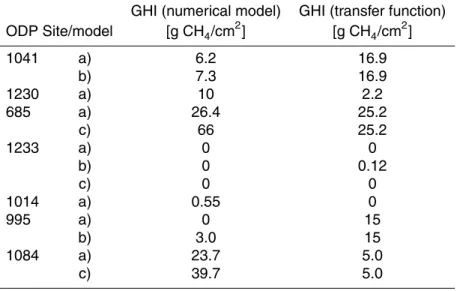
In addition, the function has been applied to the ODP Sites of Costa Rica, Peru, Chile, California, Blake Ridge and Namibia, which are presented in Sect. 2. The re-sults are listed in Table 3. The GH amounts calculated with the transfer function are

all between 0 and 25 g of CH₄/cm2 and are consistent with the results of the

ODP-20

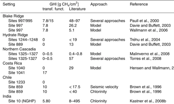
Site models without the additional upward fluid flow. Additionally, the validity of the transfer function was tested by comparing its results with several published studies based on direct observations, geochemical modelling and other methods (resistivity logs, chlorinity anomalies, and seismic velocity analysis; Table 4). Overall, the GH con-centrations obtained with the transfer function are in good accordance with the results 25

(18)

BGD

7, 1057–1099, 2010

M. Marquardt et al.

Title Page

Tables Figures

◭ ◮

Back Close

Full Screen / Esc

(ODP Leg 311) or Blake Ridge (Table 4). The transfer function does not predict any GH for Hydrate Ridge, which is in line with results of Torres et al. (2004) and Tr ´ehu et al. (2004) who state that strong GH enrichments at the summit (Sites 1249–1250) are due to enhanced gas flux. Away from the summit (Sites 1244–1248) there is almost no indication for GH formation.

5

Kastner et al. (2008b) estimated GH concentrations from 8 to 495 g of CH₄/cm2(1 to

61 vol.%) at the Indian continental margin (Site 10). Assuming that the lower concen-trations display the regional background concentration of GH, the amount calculated

by the transfer function of 5.4 g of CH₄/cm2 is in good accordance with the minimum

potential GH at this site. 10

An estimate of 29 g of CH₄/cm2was made for Site 1040 o_ffshore Costa Rica (Hensen

and Wallmann, 2005) applying a geochemical model which considers fluid flow and a

different kinetic approach for POC degradation. However, the transfer function does

not predict any GH at this site considering a POCar of 2.3 g/m2/yr, because of the low

sediment thickness above the d ´ecollement (380 m). Indeed at Site 1041 and with a 15

sediment thickness of 750 m within the GHSZ, the function gives an amount of 17 g of

CH₄/cm2, which is still in the expected range.

It should be noted that the function gives lower GHI values than obtained by other methods at high gas flux sites since the ascent of methane with rising fluids and gases is not considered in the model. These additional transport pathways are presently not 20

included in the transfer function because fluid and gas flow are strongly variable in

space and time, and hence very difficult to constrain and to generalise. At present, the

function predicts the potential of GH formation via biogenic CH₄ formation within the

GHSZ, only.

6 Conclusions

25

(19)

BGD

7, 1057–1099, 2010

M. Marquardt et al.

Title Page

Tables Figures

◭ ◮

Back Close

Full Screen / Esc

The derived transfer function is based on two ubiquitously available parameters, the POC accumulation rate (POCar) and the thickness of the gas hydrate stability zone (GHSZ). Hence, we provide a simple prognostic tool for GH quantification in marine sediments which enables the estimation of GH inventories formed by in situ produced

CH₄ without the need of detailed information concerning the geological condition or

5

running complex numerical models. Hence, the extrapolation to regional scales is com-paratively simple.

It must be pointed out that the transfer function does not account for e_ffects of fluid

advection and methane gas ascent (HGF sites), which means that it will typically predict minimum estimates. However, at low gas flux sites (LGF) sites, which represent the 10

most common setting on a global scale, testing the function has shown that reasonable GH inventories are predicted.

Appendix A

Rate laws and boundary conditions 15

See Tables A1 and A2.

Acknowledgements. This work has been supported by the DFG financed project HYDRA and the Kiel-based SFB 574 and by the BMBF-financed SUGAR project.

References

Archer, D., Buffett, B., and Brovkin, V.: Ocean methane hydrates as a slow tipping point in

20

the global carbon cycle, P. Natl. Acad. Sci. USA, Special Feature, 106(49), 20596–20601, doi:10.1073/pnas.0800885105, 2008.

(20)

BGD

7, 1057–1099, 2010

M. Marquardt et al.

Title Page

Tables Figures

◭ ◮

Back Close

Full Screen / Esc

Interactive Discussion Berner, R. A.: Early Diagenesis – A Theoretical Approach, Princeton University Press,

Prince-ton, USA, 1980.

Bhatnagar, W., Chapman, G., Dickens, G. R., Dugan, B., and Hirasaki, G. J.: Generalization of gas hydrate distribution and saturation in marine sediments by scaling of thermodynamic and transport processes, Am. J, Sci., 307, 861–900, 2007.

5

Brown, K. M., Bangs, N. L., Froelich, P. N., and Kvenvolden, K. A.: The nature, distribution and origin of gas hydrate in the Chile triple junction region, Earth Planet. Sc. Lett., 139, 471–483, 1996.

Brown, H. E., Holbrook, W. S., Hornbach, M. J., and Nealon, J.: Slide structure and role of gas hydrate at the northern boundary of the Storegga Slide, offshore Norway, Mar. Geol., 229,

10

179–186, 2006.

Buffett, B. A. and Archer, D.: Global inventory of methane clathrate: sensitivity to changes in the deep ocean, Earth Planet. Sc. Lett., 227, 185–199, 2004.

Burdige, D. J.: Preservation of Organic Matter in Marine Sediments: Controls, Mechanisms, and an Imbalance in Sediment Organic Carbon Budgets, Chem. Rev., 107, 476–485, 2007.

15

Chand, S., Minshull, T. A., Gei, D., and Carcione, J. M.: Elastic velocity models for gas-hydrate-bearing sediments – a comparison, Geophys. J. Int., 159, 573–590, 2004.

Chave, A. D. and Cox, C. S.: Controlled Electromagnetic Sources for Measuring Electrical Conductivity beneath the Oceans 1. Forward Problem and Model Study, J. Geophys. Res., 87(B0), 5327–5383, 1982.

20

Colman A. S. and Holland H. D.: The global diagenetic flux of phosphorus from marine sedi-ments to the oceans: Redox sensitivity and the control of atmospheric oxygen levels. Special Publication, Society for Sedimentary Geology, 66, 53–75, 2000.

D’Hondt, S. L., Jørgensen, B. B., Miller, D. J., Aiello, I. W., Bekins, B., Blake, R., Cragg, B. A., Cypionka, H., Dickens, G. R., Ferdelman, T., Ford, K. H., Gettemy, G. L., Gu `erin, G.,

25

Hinrichs, K.-U., Holm, N., House, C. H., Inagaki, F., Meister, P., Mitterer, R. M., Naehr, T. H., Niitsuma, S., Parkes, R. J., Schippers, A., Skilbeck, C. G., Smith, D. C., Spivack, A. J., Teske, A., Wiege, J.: Controls on microbial communities in deeply buried sediments, eastern Equatorial Pacific and Peru margin, Sites 1225–1231, Proceedings of the Ocean Drilling Program, Initial Reports, 201, 2003.

30

Davie, M. K. and Buffett, B. A.: A numerical model for the formation of gas hydrate below the seafloor, J. Geophys. Rev., 106(B1), 497–514, 2001.

(21)

BGD

7, 1057–1099, 2010

M. Marquardt et al.

Title Page

Tables Figures

◭ ◮

Back Close

Full Screen / Esc

Interactive Discussion a comparison of observations and numerical models, Earth Planet. Sc. Lett., 206, 51–63,

2003.

Dickens, G. R., O’Neil, J. R., Rea, D. K., and Owen, R. M.: Dissociation of oceanic methane hy-drate as a cause of the carbon isotope excursion at the end of the Paleocene, Paleoceanogr. Currents, 10(6), 965–971, 1995.

5

Dickens, G. R., Paull, C. K., Wallace, P., and the ODP Leg 164 Scientific Party: Direct measure-ment of in situ methane quantities in a large gas-hydrate reservoir, Nature, 385, 426–428, 1997.

Dickens, G. R. and Snyder, G. T.: Interpreting upward methane flux from marine pore water profiles, Fire In The Ice, Winter, Methane Hydrate Newsletter, published by US Department

10

of Energy, Office of Fossil Energy, National Energy Technology Laboratory, 7–10, 2009. Dobrynin, V., Korotajev, Y., and Plyuschev, D.: Gas Hydrates: A Possible Energy Resource,

in: Long-Term Energy Resources, edited by: Meyer, R. and Olson, J., Boston, MA, Pitman, 727–729, 1981.

Egeberg, P. K. and Dickens, G. R.: Thermodynamic and pore water halogen constraints in gas

15

hydrate distribution at ODP Site 997 (Blake Ridge), Chem. Geol., 153, 53–79, 1999.

Ersland, G., Husebø, J., Graue, A., and Kvamme, B.: Transport and storage of CO2 in natural gas hydrate reservoirs, Energy Procedia, 1, 3477–3484, 2009.

Ford, K. H., Naehr, T. H., Skilbeck, C. G., and the Leg 201 Scientific Party: The use of infrared thermal imaging to identify gas hydrate in sediment cores, in: Proceedings of the Ocean

20

Drilling Program, edited by: D’Hondt, S. L., Jørgensen, B. B., Miller, D. J ., et al., Initial Reports, 201, 1–20, 2003.

Haeckel, M., Suess, E., Wallmann, K., and Rickert, D.: Rising methane gas bubbles form mas-sive hydrate layers at the seafloor, Geochim. Cosmochim. Ac., 68(21), 4335–4345, 2004. Heeschen, K. U., Hohnberg, H. J ., Haeckel, M., Abegg, F., Drews, M., and Bohrmann, G.: In

25

situ hydrocarbon concentration from pressurised cores in surface sediments, Northern Gulf of Mexico, Mar. Chem., 107, 498–515, 2007.

Hensen, C. and Wallmann, K.: Methane formation at Costa Rica continental margin - con-straints for gas hydrate inventories and cross-d ´ecollement fluid flow, Earth Planet. Sc. Lett., 236, 41–60, 2005.

30

(22)

BGD

7, 1057–1099, 2010

M. Marquardt et al.

Title Page

Tables Figures

◭ ◮

Back Close

Full Screen / Esc

Interactive Discussion Hustoft, S., Bunz, S., Mienert, J., and Chand, S.: Gas hydrate reservoir and active

methane-venting province in sediments on<20 Ma young oceanic crust in the Fram Strait, offshore NW-Svalbard, Earth Planet. Sc. Lett., 284(1–2), 12–24, doi:10.1016/j.epsl.2009.03.038, 2009.

Hyndman, R. D., Yuan, T., and Moran, T. Y.: The concentration of deep sea gas hydrates

5

from downhole electrical resistivity logs and laboratory data, Earth Planet. Sc. Lett., 172, 167–177, 1999.

Kastner, M., Torres, M., Solomon, E., and Spivack, A. J.: Marine Pore Fluid Profiles of Dissolved Sulfate; Do They Reflect In Situ Methane Fluxes?, Fire In The Ice, Summer, Methane Hydrate Newsletter, published by US Department of Energy, Office of Fossil Energy, National Energy

10

Technology Laboratory, 6–8, 2008a.

Kastner, M., Spivack, A. J., Torres, M., Solomon, E., Borole, D. V., Robertson, G., and Das, H. C.: Gas hydrates in three Indian ocean regions, a comparative study of occurrence and subsurface hydrology, Proceedings of the 6th International Conference on Gas Hydrates (ICGH 2008), Vancouver, British Columbia, Canada, 2008b.

15

Kennett, J. P., Cannariato, K. G., Hendy, I. L., and Behl, R. J.: Methane Hydrates in Quaternary Climate Change, The Clathrate Gun Hypothesis, American Geophysical Union, Washington, DC, 216 pp., 2003.

Kimura, G., Silver, E., Blum, P., et al.: Proceedings of the Ocean drilling Programm, Initial Reports, 170, College Station, TX, 458 pp., 1997.

20

Klauda, J. B. and Sandler, S. I.: Global Distribution of Methane Hydrate in Ocean Sediment, Energ. Fuel, 19, 459–470, 2005.

Kvenvolden, K. A.: Methane hydrates - a major reservoir of carbon in the shallow geosphere?, Chem. Geol., 71, 41–51, 1988.

Liu, X. and Flemmings, P. B.: Dynamic multiphase flow model of hydrate formation in marine

25

sediments, J. Geophys. Rev., 112, B03101, doi:10.1029/2005JB004227, 2007.

Malinverno, A., Kastner, M., Torres, M. E., and Wortmann, U. G.: Gas hydrate occurrence from pore water chlorinity and downhole logs in a transect across the northern Cascadia margin (Integrated Ocean Drilling Program Expedition 311), J. Geophys. Res., 113, B08103, doi:10.1029/2008JB005702, 2008.

30

Middelburg, J.: A simple rate model for organic matter decomposition in marine sediments, Geochim. Cosmochim. Ac., 53, 1577–1581, 1989.

(23)

BGD

7, 1057–1099, 2010

M. Marquardt et al.

Title Page

Tables Figures

◭ ◮

Back Close

Full Screen / Esc

Interactive Discussion out there?, Earth Sci. Rev., 66, 183–197, 2004.

Milkov, A. V.: Molecular and stable isotope compositions of natural gas hydrates: A revised global dataset and basic interpretations in the context of geological settings, Org. Geochem., 36(5), 681–702, 2005.

Mix, A. C., Tiedemann, R., Blum, P., et al.: Proceedings of the Ocean Drilling Program, Initial

5

Reports, 202, 2003.

Moridis, G. J., Collett, T. S., Dallimore, S. R., Satoh, T., Hancock, S., and Weatherill, B.: Numer-ical studies of gas production from several CH4hydrate zones at the Mallik site, Mackenzie

Delta, Canada, J. Petrol. Sci. Eng., 43, 219–238, 2004.

Paull, C. K., Matsumoto, R., Wallace, P. J., et al.: Proceedings of the Ocean Drilling Program,

10

Initial Reports, Vol. 164, 1996.

Paull, C. K., Matsumoto, R., Wallace, P. J., and Dillon, W. P. (eds.): Proc. ODP, Sci. Results, 164: College Station, TX (Ocean Drilling Program), 2000.

Pollack, H. N., Hurter, S. J., and Johnson, J. R.: Heat Flow from the Earth’s Interior: Analysis of the Global Data Set, Rev. Geophys., 31(3), 267–280, 1993.

15

Riedel, M., Willoughby, E. C., Chen, M. A., He, T., Novosel, I., Schwalenberg, K., Hyn-dman, R. D., Spence, G. D., Chapman, N. R., and Edwards, R. N.: Gas hydrate on the northern Cascadia margin: regional geophysics and structural framework, edited by: Riedel, M., Collett, T. S., Malone, M. J., and the Expedition 311 Scientists, Proc. IODP, 311, Washington, DC (Integrated Ocean Drilling Program Management International, Inc.),

20

doi:10.2204/iodp.proc.311.109.2006, 2006.

Schwalenberg, K., Willoughby, E., Mir, R., and Nigel Edwards, R.: Marine gas hydrate electro-magnetic signatures in Cascadia and their correlation with seismic blank zones, First Break, 23, Special Topic, Petroleum Geology, 57–63, 2005.

Seiter, K., Hensen, C., Schr ¨ote, J., and Zabel, M.: Organic carbon content in surface sediments

25

– defining regional provinces, Global Biogeochem. Cy, GB1010, 1–26, 2004.

Sloan, E. D. and Koh, C. A.: Clathrate hydrates of natural gases, Chapter Hydrate Dissociation, in Chemical Industries/119, 3.edit., CRC Press, New York, USA, 752 pp., 2007.

Soloviev, V. A.: Global estimation of gas content in submarine gas hydrate accumulations, Russ. Geol. Geophys., 43, 609–624, 2002.

30

(24)

BGD

7, 1057–1099, 2010

M. Marquardt et al.

Title Page

Tables Figures

◭ ◮

Back Close

Full Screen / Esc

Interactive Discussion solubility of methane hydrate in seawater, Chem. Geol., 219, 37–52, 2005.

Torres, M. E., Wallmann, K., Tr ´ehu, A. M., Bohrmann, G., Borowski, W. S., and Tomaru, H.: Gas hydrate growth, methane transport, and chloride enrichment at the southern summit of Hydrate Ridge, Cascadia margin offOregon, Earth Planet. Sc. Lett., 226, 225–241, 2004. Torres, M. E., Tr ´ehu, A. M., Cespedes, N., Kastner, M., Wortmann, U. G., Kim, J. H., Long,

5

P., Malinverno, A., Pohlman, J. W., Riedel, M., and Collett, T.: Methane hydrate formation in turbidite sediments of northern Cascadia, IODPExpedition 311, Earth Planet. Sc. Lett., 271, 170–180, 2008.

Tr ´ehu, A. M., Torres, M. E., Long, P. E., Torres, M. E., Bohrmann, G., Rack, F. R , Collet, T. S., Goldberg, D. S. , Milkov, A. V., Riedel, M., Schultheiss, P., Bangs, N. L., Barr, S. R.,

10

Borowski, W. S., Claypool, G. E., Delwiche, M. E., Dickens, G. R., Gracia, E., Guerin, G., Holland, M. , Johnson, J. E., Lee, Y.-J., Liu, C.-S., Su, X., Teichert, B., Tomaru, H., Vanneste, M., Watanabe, M., and Weinberger, J. L.: Three-dimensional distribution of gas hydrate beneath southern Hydrate Ridge: constraints from ODP Leg 204, Earth Planet. Sc. Lett., 222, 845–862, 2004.

15

Tromp, T. K., Van Cappellen, P., and Key, R. M.: A global model for the early diagenesis of organic carbon and organic phosphorus in marine sediments, Geochim. Cosmochim. Ac., 59(7), 1259–1284, 1995.

Uchida, T., Lu, H., Tomaru, H. and the MITI Nankai Trough Shipboard Scientists: Sub-surface Occurrence of Natural Gas Hydrate in the Nankai Trough Area: Implication for

20

Gas Hydrate Concentration, in: Resource Geologym., 54, 35–44, doi:10.1111/j.1751-3928.2004.tb00185.x, 2004.

Wallmann, K., Aloisi, G. Haeckel, M., Obzhirov, A., Pavlova, G., and Tishchenko, P.: Kinetics of organic matter degradation, microbial methane generation, and gas hydrate formation in anoxic marine sediments, Geochim. Cosmochim. Ac., 70, 3905–3927, 2006.

25

Westbrook, G. K., Chand, S., Rossi, G., Long, C., B ¨unz, S., Camerlenghi, A., Caricione, J. M., Dean, S., Foucher, J.-P., Flueh, E., Gei, D., Haacke, R. R., Madrussane, G., Mienert, J., Minshull, T. A., Nouz ´e, H., Peacock, S., Reston, T. J., Vanneste, M., and Zillmer, M.: Estimation of gas hydrate concentration from multi-component seismic data at sites on the continental margins of NW Svalbard and the Storegga region of Norway, Mar. Petrol. Geol.,

30

25, 744–758, 2008.

(25)

BGD

7, 1057–1099, 2010

M. Marquardt et al.

Title Page

Tables Figures

◭ ◮

Back Close

Full Screen / Esc

Interactive Discussion Xu, W. and Germanovich, L. N.: Excess pore pressure resulting from methane hydrate

dis-sociation in marine sediments: A theoretical approach, J. Geophys. Res., 111, BO1104, doi:10.1029/2004JB003600, 2006.

Yuan, T., Hyndman, R. D., Spence, G. D., and Desmons, B.: Seismic velocity increase and deep-sea gas hydrate concentration above a bottom-simulating reflector on the nothern

Cas-5

cadia continental slope, J. Geophys. Res., B101, 13655–13671, 1996.

(26)

BGD

7, 1057–1099, 2010

M. Marquardt et al.

Title Page

Tables Figures

◭ ◮

Back Close

Full Screen / Esc

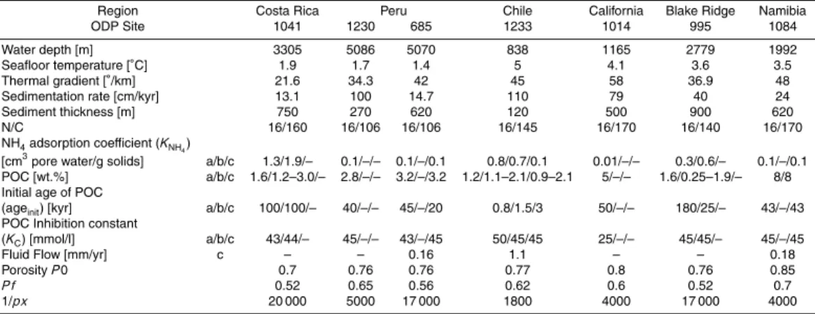
Table 1.Parameters, constants and coefficients of the modelled ODP Sites 1041 (Costa Rica), 685 and 1230 (Peru), 1233 (Chile), 1014 (California), 995 (Blake Ridge), and 1084 (Namibia). The varying values for the different model runs (constant POC input, varying POC input and fluid flow) are listed as a, b, and c. The porosity is calculated after Berner (1980) with the porosity at the surface (P0), at the lower boundary (P f) and the coefficient for the decrease of porositypx.

Region Costa Rica Peru Chile California Blake Ridge Namibia

ODP Site 1041 1230 685 1233 1014 995 1084

Water depth [m] 3305 5086 5070 838 1165 2779 1992

Seafloor temperature [◦_C] _1.9 _1.7 _1.4 ₅ _4.1 _3.6 _3.5

Thermal gradient [◦_/km] _21.6 _34.3 ₄₂ ₄₅ ₅₈ _36.9 ₄₈

Sedimentation rate [cm/kyr] 13.1 100 14.7 110 79 40 24

Sediment thickness [m] 750 270 620 120 500 900 620

N/C 16/160 16/106 16/106 16/145 16/170 16/140 16/170

NH4adsorption coefficient (KNH4)

[cm3_{pore water/g solids]} _a/b/c _1.3/1.9/– _0.1/–/– _0.1/–/0.1 _0.8/0.7/0.1 _0.01/–/– _0.3/0.6/– _0.1/–/0.1

POC [wt.%] a/b/c 1.6/1.2–3.0/– 2.8/–/– 3.2/–/3.2 1.2/1.1–2.1/0.9–2.1 5/–/– 1.6/0.25–1.9/– 8/8

Initial age of POC

(ageinit) [kyr] a/b/c 100/100/– 40/–/– 45/–/20 0.8/1.5/3 50/–/– 180/25/– 43/–/43

POC Inhibition constant

(KC) [mmol/l] a/b/c 43/44/– 45/–/– 43/–/45 50/45/45 25/–/– 45/45/– 45/–/45

Fluid Flow [mm/yr] c – – 0.16 1.1 – – 0.18

PorosityP0 0.7 0.76 0.76 0.77 0.8 0.76 0.85

P f 0.52 0.65 0.56 0.62 0.6 0.52 0.7

(27)

BGD

7, 1057–1099, 2010

M. Marquardt et al.

Title Page

Tables Figures

◭ ◮

Back Close

Full Screen / Esc

Table 2. Input parameters and boundary conditions for the standard model using average values of all specific ODP models. The range of parameter values used for the sensitivity analysis are also shown.

Standard model Sensitivity (average of ODP models) analysis

Thermal gradient [ ˚ /km] 44.2 10–65

Seafloor temperature [ ˚ C] 3.1 1–6

Water depth [m] 2516 500–5500

GHSZ [m] 450 50–2000

POC accumulation rate [g/m2/yr] 4.3 0.7–40

– POC input [wt.%] 2.3 1.2–3.1

– Sedimentation rate [cm/kyr] 32 9.5–200

Initial age of POC [kyr] 43.7 43.7

Inhibition constant of

(28)

BGD

7, 1057–1099, 2010

M. Marquardt et al.

Title Page

Tables Figures

◭ ◮

Back Close

Full Screen / Esc

Table 3.Comparison of the GH amounts of the ODP sites calculated in the different model runs:

(a)constant POC input,(b)varying POC input, (c)time-dependent POC input and advective fluid flow, with the transfer function, using the input data of the ODP models.

GHI (numerical model) GHI (transfer function) ODP Site/model [g CH4/cm

2

] [g CH4/cm 2

]

1041 a) 6.2 16.9

b) 7.3 16.9

1230 a) 10 2.2

685 a) 26.4 25.2

c) 66 25.2

1233 a) 0 0

b) 0 0.12

c) 0 0

1014 a) 0.55 0

995 a) 0 15

b) 3.0 15

1084 a) 23.7 5.0

(29)

BGD

7, 1057–1099, 2010

M. Marquardt et al.

Title Page

Tables Figures

◭ ◮

Back Close

Full Screen / Esc

Table 4.Comparison of the GHI amount calculated with the transfer function to other published results obtained from several approaches, such as seismic velocity calculations, chlorinity, re-sistivity log or a combination of several of these methods. Other results obtained by numerical modelling are also shown.

Setting GHI [g CH₄/cm2] Approach Reference transf. funct. Literature

Blake Ridge

Sites 997/995 7.8/15 48–97 Several approaches Paull et al., 2000

Site 997 7.8 26.2 Model Davie and Buffett, 2003

Site 997 7.8 5.1 Model Wallmann et al., 2006

Hydrate Ridge

Sites 1244–1248 0 <19 Several approaches Tr ´ehu et al., 2004

Site 889 0 13 Model Davie and Buffett, 2003

Northern Cascadia

Sites 1325–1327 0–0.5 0.4–0.8 Model Malinverno et al., 2008 Sites 1325-1327 0–0.5 57 Several approaches Torres et al., 2008 Costa Rica

Site 1040 0 29 Model Hensen and Wallmann, 2005

Site 1041 17 Chile

Site 1233 0

Site 859 10 <17.5 Seismic velocity Brown et al., 1996 Site 859 10 <40 Chlorinity Brown et al., 1996 India

(30)

BGD

7, 1057–1099, 2010

M. Marquardt et al.

Title Page

Tables Figures

◭ ◮

Back Close

Full Screen / Esc

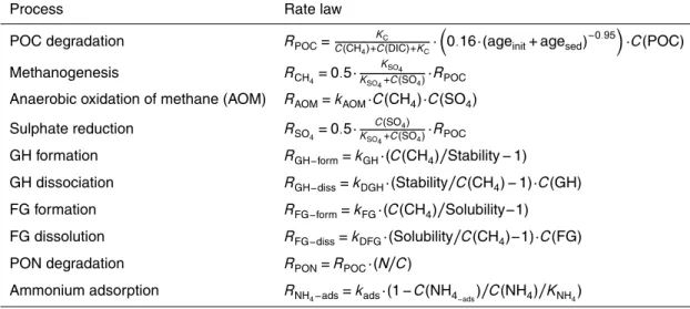
Table A1. Summary of the main rate laws.

Process Rate law

POC degradation RPOC=

KC

C(CH4)+C(DIC)+KC·

0.16·(ageinit+agesed)−0.95

·C(POC)

Methanogenesis RCH₄=0.5·_K KSO4

SO4+C(SO4)·RPOC Anaerobic oxidation of methane (AOM) RAOM=kAOM·C(CH4)·C(SO4)

Sulphate reduction RSO4=0.5·

C(SO4)

K_SO4+C(SO4)·RPOC

GH formation RGH−form=kGH·(C(CH4)/Stability−1)

GH dissociation RGH−diss=kDGH·(Stability/C(CH4)−1)·C(GH)

FG formation RFG−form=kFG·(C(CH4)/Solubility−1)

FG dissolution RFG−diss=kDFG·(Solubility/C(CH4)−1)·C(FG)

PON degradation RPON=RPOC·(N/C)

(31)

BGD

7, 1057–1099, 2010

M. Marquardt et al.

Title Page

Tables Figures

◭ ◮

Back Close

Full Screen / Esc

Table A2. Boundary conditions and constants used for the ODP model. Nomenclature after Wallmann et al. (2006).

Parameter/Coefficient Value

Kinetic constant for AOM (kAOM)1/(mmol/cm 3

/yr) 1

Kinetic constant for NH4adsorption (kads) [mmol/cm 3

/yr] 0.0001 Density of dry solids [g/cm3] 2.5 Monod constant for SO4reduction (kSO4) [mmol/cm

3

] 0.001 Kinetic constant for GH precipitation (k_GH) [wt.%/yr] 0.005 Kinetic constant for GH dissolution (k_DGH) [1/yr] 0.02 Kinetic constant for FG precipitation (k_FG) [vol.%/yr] 0.5 Kinetic constant for FG dissolution (k_DFG) [1/yr] 0.5 SO4concentration upper/lower boundary [mmol/l] 28/0

CH4concentration upper boundary [mmol/l] 0

(32)

BGD

7, 1057–1099, 2010

M. Marquardt et al.

Title Page Abstract Introduction Conclusions References Tables Figures ◭ ◮ ◭ ◮ Back Close

Full Screen / Esc

Dob ryni

n et al. (198 1) Kve nvol den and Cla ypoo

l (19 88)

Gor nitz

and Fun

g (1 994) Mak ogon (199 7) Solo viev (200 2) Milk ov (2

004)

Buf fet a

nd A rche

r (2 004) Kla uda and Sand ler (200 5) Dic kens (200 1) 1x1016 1x1017 1x1018 1x1019 1x1020 1x1021 1x1022 G H [ g C H4 ] 1x1016 1x1017 1x1018 1x1019 1x1020 1x1021 G H [ g C ]

Global estimates of GH in marine sediments Kla uda and Sand ler (200 5)

Fig. 1. Selected estimates of global GH inventories since the early 1980’s. The quantities range over 5 orders of magnitude from 1017to 1022g of CH4. At present, an inventory of about

4×1018g of CH4(3000 Gt C) estimated by Buffett and Archer (2004) seems to be the most likely

scenario.

(33)

BGD

7, 1057–1099, 2010

M. Marquardt et al.

Title Page

Tables Figures

◭ ◮

Back Close

Full Screen / Esc

Interactive Discussion 0 0.25 0.5 0.75 1

0 4 8 12 0 0.1 0.2 0.3

0 1 2 3 0 40 80 120 160

800 600 400 200 0

D

ep

th

[

m

]

0 0.25 0.5 0.75 1 GH [vol.%] 0 4 8 12

NH4 [mmol/l] 0 0.1 0.2 0.3

PON [wt.%] 0 1 2 3

POC [wt.%]

GH + CH4

CH4

0 40 80 120 160 SO4 / CH4 [mmol/l]

800 600 400 200 0

D

e

p

th

[

m

]

a) - const. POC - no fluid flow

b) - var. POC - no fluid flow ODP Site 1041

GH = 0.21 vol.% GHI = 6.2 g CH4/cm2

GH = 0.24 vol.% GHI = 7.3 g CH4/cm2

GH + CH4

CH4

Fig. 2.Model results for ODP Site 1041 offCosta Rica for two different model runs:(a)constant POC input, and(b)varying POC input over time. In the GH plot the average GH concentration (in % of the pore space) and the integrated GHI amount (in g CH4/cm

2

) are given.