www.hydrol-earth-syst-sci.net/16/357/2012/ doi:10.5194/hess-16-357-2012
© Author(s) 2012. CC Attribution 3.0 License.
Earth System
Sciences
Physically-based modeling of topographic effects on spatial
evapotranspiration and soil moisture patterns through radiation
and wind
M. Liu1,2, A. B´ardossy3, J. Li4, and Y. Jiang1
1State Key Laboratory of Earth Surface Processes and Resource Ecology, Beijing Normal University, Beijing, China 2Helmholtz Research Centre for Environment, Magdeburg, Germany
3Institute of Modelling Hydraulic and Environmental Systems, University Stuttgart, Stuttgart, Germany 4School of Civil, Environmental and Mining Engineering, the University of Adelaide, Adelaide, Australia Correspondence to: M. Liu ([email protected])
Received: 23 June 2011 – Published in Hydrol. Earth Syst. Sci. Discuss.: 20 July 2011 Revised: 17 December 2011 – Accepted: 23 January 2012 – Published: 6 February 2012
Abstract. In this paper, simulations with the Soil Water At-mosphere Plant (SWAP) model are performed to quantify the spatial variability of both potential and actual evapotran-spiration (ET), and soil moisture content (SMC) caused by topography-induced spatial wind and radiation differences. To obtain the spatially distributed ET/SMC patterns, the field scale SWAP model is applied in a distributed way for both pointwise and catchment wide simulations. An adapted radi-ation model from r.sun and the physically-based meso-scale wind model METRAS PC are applied to obtain the spatial radiation and wind patterns respectively, which show signif-icant spatial variation and correlation with aspect and ele-vation respectively. Such topographic dependences and spa-tial variations further propagate to ET/SMC. A strong spaspa-tial, seasonal-dependent, scale-relevant intra-catchment variabil-ity in daily/annual ET and less variabilvariabil-ity in SMC can be ob-served from the numerical experiments. The study concludes that topography has a significant effect on ET/SMC in the humid region where ET is a energy limited rather than water availability limited process. It affects the spatial runoff gen-eration through spatial radiation and wind, therefore should be applied to inform hydrological model development. In addition, the methodology used in the study can serve as a general method for physically-based ET estimation for data sparse regions.
1 Introduction
Evapotranspiration (ET) is a very important element in hy-drological cycle, and it is adopted as the criteria for climate classification (Thornthwaite and Mather, 1955). Globally ET amounts to more than 60 % of the precipitation that falls on the continents (Dingman, 2002), and in arid and semi-arid gions, it is much higher. At long-term, ET determines the re-gional water balance and hydro-ecological system, whereas at short-term, it affects the crop growth and yield, as well as the antecedent moisture conditions (AMC) which controls the rainfall-runoff generation processes, thus the hydrologi-cal response of the catchment. For most climate conditions, soil moisture content (SMC) and ET are strongly coupled together, and they are the key variables for soil water bud-get, which helps to optimize water balance management or forecast flash floods (Cassardo et al., 2002; Norbiato et al., 2008). Temporal ET and SMC dynamics also has a strong implication on the interpretation of global climate change.
Crave, 1997, etc.) suggest that lateral water redistribution in unsaturated and saturated zone is the major driving force for spatial soil moisture distribution. Lateral soil-water flow is independent from the ET process and can be described with the approach based on topographic index (Beven and Kirkby, 1979). However, Western et al. (1999) have found that lateral water redistribution is dominant only under wet conditions, while under dry conditions radiation which drives the verti-cal water transfer is more crucial. In the vertiverti-cal direction, SMC is strongly coupled with ET, with the spatial patterns of both being subjected to spatial soil, vegetation and meteo-rological variabilities (El Maayar and Chen, 2006; Mohanty and Skaggs, 2001), which are to certain extent, related to to-pography. Jenny (1941) has given the well-known factors of
soil formation, including climate, biota, topography and
par-ent material and time, which has been validated by numerous case studies (Florinsky et al., 2002; Odeh et al., 1994). Stud-ies have also confirmed the dependence of vegetation pattern on topography, climate and soil (Ostendorf and Reynolds, 1998; Schr¨oder, 2006; Reed et al., 2009). However, pedoge-nesis and land cover evolution are both long-term processes and exhibit hight degree of randomness. Given that topog-raphy is a readily-available information, it is of great inter-est to quantify the spatial variability of ET/SMC that stems from topography. Sensitivity test for ET under the Mediter-ranean climate conditions by Bois et al. (2008) suggest that wind speed and solar radiation are the two most influential factors for reference ET. In this paper, we revisit the issue of spatial ET/SMC variability caused by the topographically re-lated factors acting in the vertical direction, but focus on the two shot-term and more deterministic factors, i.e. radiation and wind. In addition to the usually investigated potential or reference ET, more efforts are shed to actual ET (ETA). Here the difference among the three widely used terms, potential ETP, actual ET and reference ET, has to be clarified. ETP is originally defined as “the amount of water transpired in a given time by a short green crop, completely shading the ground, of uniform height and with adequate water status in the soil profile” by Penman (1948), and it has been general-ized to describe the maximum ET possible under specific cli-matic conditions with unlimited water availability in the soil for any vegetation. ETA is the exact water loss by soil and vegetation under water stress conditions. Reference ET is the definition adopted by FAO (1990), which refers to “the rate of evapotranspiration from a hypothetical reference crop with an assumed crop height of 0.12 m, a fixed surface resistance of 70 s m−1 and an albedo of 0.23, closely resembling the evapotranspiration from an extensive surface of green grass of uniform height, actively growing, well-watered and com-pletely shading the ground”. In this work, the term ETP in general sense and the term ETA are adopted.
In contrast to other hydrological parameters such as precipitation and temperature, reliable direct measurement of ET/SMC is more difficult and expensive. More-over, the strong spatial variation of ET/SMC to the local
meteorological and hydrological conditions, referred by Western et al. (2002) as scale effect, together with the high cost of measurements, render all types of point measure-ments impractical for spatial mapping. Remote sensing are nowadays widely deployed to measure SMC and to derive ET. However, limitations due to the interfering signal of soil surface roughness and vegetation canopy and the re-stricting signal penetration depth prevent the operational ap-plication of soil moisture remote sensing at current stage (Western et al., 2002). Alternatively, inferring ET/SMC with modeling approach using other remotely sensed parameters, such as land surface temperature (LST), vegetation index (NDVI/EVI), etc. are widely explored (Cleugh et al., 2007; Wang et al., 2007; Mu et al., 2007). Most methods are tar-geting ETP evaluation. Empirical equations based on sim-ple meteorological input(s) is one of the most commonly used approach for the estimation of regional ET. Xu and Singh (2000) provided an extensive review of the temper-ature and radiation based method. Some empirical meth-ods have been developed to utilize the remotely sensed LST and vegetation index data to calculate ETA, such as triangle method (Price, 1990), B-method (Carlson et al., 1995), tem-perature/vegetation dryness index (TVDI) (Andersen et al., 2002). A good overview of the remote-sensing based tech-niques can be found in Verstraeten et al. (2008).
More physically sound approaches are based on the con-servation of either energy, mass or both. Penman-Monteith method, also called the combination method, because it elim-inates the surface temperature and does not need an explicit calculation of sensible heat flux, is the most popular ap-proach used in modeling the physical process of ET. The sur-face energy balance method, usually applied in some land surface models (LSM), on the contrary, try to employ re-motely sensed LST data to derive aerodynamic surface tem-perature and to explicitly determine sensible heat flux, so that the latent heat flux associated with ET can be calculated as a residual (Bastiaanssen et al., 1998; Su, 2002). Jensen et al. (1990) analyzed the performance of 20 different ET formulas against lysimeter data for 11 stations around the world under different climatic conditions, and the Penman-Monteith approach is ranked as the best for all climatic con-ditions. This paper will apply the the Soil Water Atmosphere Plant (SWAP) model, which contains the Penman-Monteith approach as the core module for ET estimation, to avoid the complexity of surface temperature estimation associated typ-ically with LSMs.
the numerical experiments. Both pointwise and spatial sim-ulations are performed. The pointwise experiment examines the effect of soil on ET/SMC variability in addition to the effects of solar radiation and wind. The effects of radiation, wind and their interaction are tested in three numerical exper-iments by different combinations of inputs. The experiment with actual land use (LU) is to approximate the topographic induced ET/SMC variability under the most realistic condi-tions. The results are presented statistically followed by a discussion.
2 Study area and data
2.1 Study area
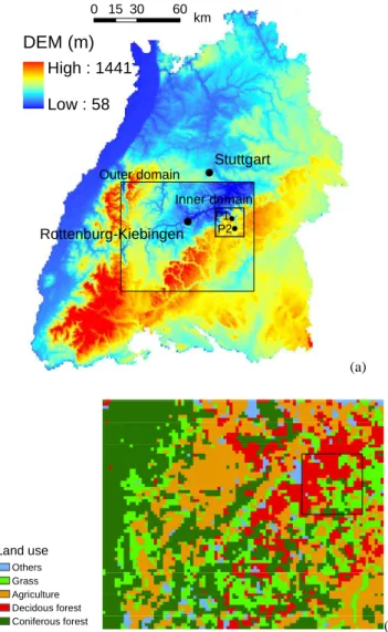
The study is focusing on the topographic effects on ET/SMC, specifically water exchange and transfer in the vertical di-rection, while neglecting the horizontal/lateral water redis-tribution. For such purpose, a delineated water basin is not necessary. Instead, a region with rich topographic features, i.e. an area with so-called complex terrain, is required to re-flect a wide range of topographic effects. In this paper, a 93×76 km2rectangular region containing both mountainous area and flood plain in the state Baden-Wuerttemberg, south-ern Germany is taken as the study area (see the outer domain in Fig. 1). A smaller area of 20×20 km2 in the northeast (the inner domain) is studied in comparison to the outer do-main to investigate the scale effects. The outer dodo-main and the inner domain are simulated at 1000 m and 100 m reso-lution respectively. The Black Forest on the western bor-der of the study area consists of crystalline bedrock whereas karstic limestone is frequently found in the eastern part of the study area. Both hill chains are characterized by steeper slopes and soils with low storage capacity. The river valleys and plains in the northern part mostly consist of thick, fertile soils. The climate can be characterized as temperate humid, with a long-term average annual precipitation of 950 mm for the state, varying from 700 mm to 1680 mm, with higher pre-cipitation in the mountainous regions and lower in the flat areas.
2.2 Meteorological data
For the numerical experiments in this study, the year 2002 with a mean annual precipitation of 970 mm for the state and 1100 mm for the study region which can be consid-ered as the average climate conditions, is taken. Daily precipitation and temperature data are obtained at the sta-tion Rottenburg-Kiebingen from German Weather Service (DWD). Both daily maximum, minimum and mean temper-ature are available. As the station does not provide humidity data, it is obtained from the nearest meteorological station Stuttgart. Humidity can also be estimated from temperature data with empirical formulas as shown by Thornton et al. (1997). Station radiation and wind data are also available at
! !
! !
Rottenburg-Kiebingen
Stuttgart
P2 P1
0 15 30 60
km
DEM (m)
High : 1441
Low : 58
Inner domain Outer domain
(a)
Land use
Others Grass Agriculture Decidous forest
Coniferous forest (b)
Fig. 1. Study area and reclassified land cover in the study area. (a) Study area and (b) land use in the study area.
the station Stuttgart for the period from 2002 to 2007, which are used to calibrate the radiation and wind models.
2.3 Land use and LAI
0 50 100 150 200 250 300 350 0
1 2 3 4 5 6 7
Day number
LAI [
−
]
(a)
0 50 100 150 200 250 300 350
0 1 2 3 4 5
Day number
LU specific LAI [
−
]
others grass agriculture deciduous coniferous
(b)
Fig. 2. Cell-based LAI at two randomly selected points with grass cover (a) and land use specific LAI for 5 different vegetation covers (b).
3 Models
To reflect the spatial ET/SMC variability, the first step is to model the spatial radiation and wind patterns. In this research, an adapted r.sun model and the mesoscale ME-TRAS PC model are applied to simulate the daily radiation and wind patterns respectively. These patterns are used then to drive the SWAP model to obtained ET/SMC fields. 3.1 Radiation model r.sun
The original r.sun model is a module for modeling of di-rect, diffuse and reflected shortwave radiation based on topographic properties in the GRASS open GIS software (Hofierka and Suri, 2002). The model can not only reflect ge-ometrical solar-earth-surface relationship for calculating the extraterrestrial radiation, but also considers the atmospheric attenuation to obtain potential radiation under clear-sky con-ditions. It can also account for cloud overcast to estimate the actual radiation, if cloud parameters such as the clear-sky in-dex (Kasten, 1983) can be provided to the model. Liu et al. (2011) have adapted the r.sun model to a stand-along pro-gram implemented together with the remote-sensing based Heliosat-2 Rigollier et al. (2004) approach to parameterize cloud. The Heliosat-2 method applies the albedo data derived from the satellite, i.e. Meteosat VIS (visible spectrum range from 0.5 to 0.9 µm) band images to estimate the clear-sky index (Cano et al., 1986; Rigollier et al., 2004). The model has been tested for three stations in Baden-Wuerttemberg and achieved an averageR2above 0.9. In this paper, daily actual radiation patterns are obtained with the adapted r.sun model.
3.2 Wind model METRAS PC
METRAS PC is the PC version of the MEsoscale TRAns-port and fluid (Stream) Model (METRAS) (Schl¨unzen et al., 2001), which is a three dimensional, non-hydrostatic wind
model to downscale from the geostrophic wind to local wind field. The model is capable of simulating wind, temperature, humidity, cloud- and rain-water-content, as well as pollutant concentration field over areas up to 800×800 km2with high accuracy for wind field. It applies a horizontally non-uniform but orthogonal grid and vertically a non-orthogonal terrain-following coordinate system. The model can reflects the to-pographic and land use modification of wind, e.g. shelter-ing, amplification due to wind tunnel effects etc. It is proven to be an “up-to-date” mesoscale model with complete func-tionalities for flow and transport simulation, and its capabil-ity in modeling mesoscale wind fields has been validated by numerous case studies (e.g. Wu and Schl¨unzen, 1992; Lenz et al., 2000; Schueler and Schl¨unzen, 2006). Moreover, because the model fulfills the requirements of VDI (2005) which requires a hit rate higher than 66 % compared with observed data for tunnel simulation and 95 % compared to analytical solution, it is widely adopted in practical applica-tions, such as air pollution prediction. In addition, the model has also been tested by World Meteorological Organization (WMO, Baklanov et al., 2008; Mikhail Sofiev and Miranda, 2009). In this study, the input geostrophic wind data for the study area is retrieved from NCEP/NCAR Reanalysis I data (Kalnay and Coauthors, 1996). The data is avlaiable daily for 17 pressure levels (1000∼10 mbar, some data, such as humidity, has less data levels). Following Frank and Land-berg (1997), the wind data at 850 mbar level for the year 2002 are chosen at the grid point (10.0◦E, 50.0◦N) as the synoptic inputs.
3.3 The SWAP model
to regional scale. It considers a one-dimensional column in the vertical direction, with the lower atmospheric layer be-ing the upper boundary for the model and the unsaturated zone or the upper part of the saturated zone being the bottom boundary. The bottom boundary conditions can be Dirichlet, Neumann, Cauchy or some mixed type. The soil water flow is simulated by the Richard’s Equation (Eq. 1) discretized in a implicit finite difference scheme.
δθ δt =
δ δz
K(h) (δh δz +1)
+S(h) (1)
wheret denotes time [d],zis the vertical coordinate taken as positive upwards [cm],K(h)is the hydraulic conductiv-ity [cm d−1] described by the Van Genuchten-Mualem model andS(h)is a sink term standing for the water extraction by plant roots [cm3cm−3d−1], i.e. actual transpiration (TA).
The actual transpiration is the integrated root water uptake of each root layer taking into account the reduction due to water and/or salinity stress (see Eq. 4). In absence of any stress, the total root uptake capacity equals to the potential transpiration rate.
RXp(z) =
lroot(z) 0 R
−Droot
lroot(z)dz
TP (2)
RXa(z) = αrRXp(z) (3)
TA= 0 Z
−Droot
RXa(z)dz (4)
wherelroot(z)is the root density [cm3cm−3] and RXp(z)and
RXa(z)are the potential and actual root water extraction rate
[cm d−1] at depthzrespectively. TP is the potential transpi-ration rate [cm d−1]. Drootis the root layer thickness [cm], αr is the reduction factors due to water, salinity stress and
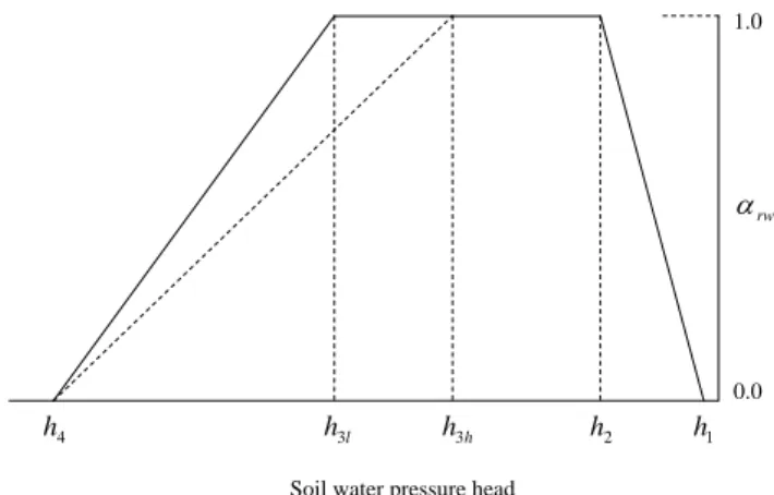
frozen conditions (dimensionless). Figure 3 shows the wa-ter stress coefficientαrwas a function of soil water pressure
head. In the rangeh3< h < h2root water uptake is optimal.
Belowh3 root water uptake linearly declines until zero at h4(permanent wilting point). The threshold pressureh3
in-creases with potential transpiration rates. For low potential transpiration TPlow, the threshold pressureh3lis lower than
the threshold pressureh3hat high potential transpiration rate
TPhigh. Aboveh2root water uptake linearly decreases due to
insufficient aeration until zero ath1.
Including TP, three potential rates are modeled by the Penman-Monteith algorithm (Eq. 5) in SWAP: potential ET of wet crop (ETPw), potential ET of dry crop (ETPd), and
potential evaporation of bare soil (EPs), based on which the
actual rates of a fully covered or non-covered surface can be calculated.
ETPd =
1v(Gn +Ln) +ρacaCat(es −ea)
ρwλv 1v +γpc 1 +CatCcan
(5)
Soil water pressure head
1
h
2
h
h
h3
l
h3 4
h
0.0 1.0
rw
D
Fig. 3. Reduction coefficient for root water uptake.
with
ET = evapotranspiration rate[LT−1]
1v= slope of the vapor pressure curve[ML−1T−3] Gn= net shortwave radiation[EL−2T−1]
Ln= net longwave radiation[EL−2T−1] ρa= air density[ML−3]
ca= heat capacity of air[EM−2T−1]
es= the saturation vapor pressure[ML−1T−2] ea= actual vapor pressure[ML−1T−2] ρw= water density[ML−3]
λv= latent heat of vaporization[EL−2T−1] γpc= psychrometric constant[ML−1T−3] Cat= atmospheric conductance[LT−1] Ccan= canopy conductance[LT−1]
The two terms in the numerator of Eq. (5) represents the two driving forces of ET: the radiation and the aerodynamic force (wind). By replacing Ccan with conductance of wet
canopy and soil, ETPwand EPs can be calculated similarly.
For partly covered soils, the potential ET of wet or dry crop is partitioned, following Eq. (6) into potential evaporation (EP) and potential transpiration (TP) which is reduced by soil cover fraction (SC) as shown in Eq. (7) or the energy interception by LAI of the vegetated area (see Eq. 8).
TP =ETPd −EP (6)
EP =(1 −SC)EPs (7)
EP =EPse−κgrLAI. (8)
Here,κgris the extinction coefficient for solar radiation. In
the SWAP model, the actual soil evaporation (EA) is deter-mined by the minimum value of EP, the restricted Darcy flux
Emaxat the top soil layer (see Eq. 9) and/or the results from
the empirical evaporation functions of Black et al. (1969) or Boesten and Stroosnijder (1986).
Emax = K1/2(θ )
h
atm −h1 −z1
z1
Here,K1/2(θ )[cm d−1] is the average hydraulic
conduc-tivity between the soil surface and the first node as a function of soil water saturationθ[−],hatmis the soil water pressure
head [cm] in equilibrium with the air relative humidity,h1is
the soil water pressure head of the first node, andz1 is the
soil depth [cm] at the first node.
The crop module of the SWAP model provides canopy condition intercepting precipitation and energy and the roots distribution function for plant uptake. The simple crop model adopted for this study prescribes crop development stage as a function of either LAI or soil cover fraction, along with crop height and rooting depth, independent of stress factors.
Infiltration excessive surface runoffqs [cm d−1] is
simu-lated with a non-linear reservoir model (see Eq. 10).
qs =
1
γsill
hpond −Zsill
βsill. (10)
The excess water on the soil surface first builds up a ponded reservoir until the pond water level hpond [cm] exceeds a
threshold ponding levelZsill [cm]. γsill[d] is the runoff
re-sistance andβsillis an exponent for the reservoir model.
Discharge from groundwater to surface water system which may consist of up to five level drainage ditches, canals or streams is described with the following general formulation:
qdrain,i =
φgwl −φdrain,i
γdrain,i
(11) whereqdrain,i[cm d−1] represents the drainage/infiltration to or from thei-th level (in this study 2 levels) of surface water system, andφdrain,i [cm] is the corresponding surface water level. φgwl [cm] is the groundwater level andγdrain,i [d] is the drainage resistance.
4 SWAP Model setup
As the focus of this research is the spatial ET/SMC variabil-ity driven by the topographically derived forces in the ver-tical direction, the effects of lateral water redistribution will be intentionally excluded by simplifying the lateral flux in the vadose zone and of groundwater. As SWAP is a one-dimensional, vertically directed model, it is best suited for this purpose. First, the model is applied to two representative plots (P1 and P2) with contrasting topographic features (see Fig. 1) to check the topographic effects by varying the radi-ation and wind inputs while keeping other factors identical. Effects of soil hydraulic properties are tested with two differ-ent soil configurations: a less permeable two-layer configu-ration of clay (soil A) on top of loam (soil B) which is typical for the region and a more permeable combination of soil C in the upper layer and soil D in the lower layer. For both cases, the upper layer is 30 cm thick with the lower layer extending to the aquitard.
To simulate the spatial ET/SMC, the SWAP model is adapted to a batch mode, running for each grid cell. Four types of spatial simulations applying different combinations of spatial and station data, referred to as numerical experi-ments because of the simplification of the soil-water regime and the application of some assumed data such as soil prop-erties, are tested in this research to investigate the effect of radiation, wind, their interaction and land use respectively:
– Experiment 1: spatial actual radiation, station wind, ho-mogeneous vegetation;
– Experiment 2: station radiation, spatial wind, homoge-neous vegetation;
– Experiment 3: spatial actual radiation, spatial wind, ho-mogeneous vegetation;
– Experiment 4: spatial actual radiation, spatial wind, ac-tual land use.
All numerical experiments, including the pairwise comparison, are conducted at two different resolutions, 100×100 m2 for the inner domain and 1×1 km2 for the outer domain to check the scale effects. The boundary condi-tions of each cell are identical except the groundwater level. A simplification of regional groundwater table is assumed – groundwater depth is linearly related to the local elevation, with a groundwater depth of 0.7 m at the lowest elevation close to the river and a depth of 1.5 m at the highest eleva-tion. This is an approximation to the TOPMODEL concept, in which the groundwater level increases with the catching area (Beven et al., 1995). A shallow groundwater aquifer of 3 m on top of an impervious aquitard is assumed for the re-gion, implying a zero bottom flux boundary. Infiltrated water from each cell reaching the groundwater table is discharged through the drainage system lying 5 cm below the groundwa-ter table directly to nearest surface wagroundwa-ter bodies and no lat-eral flux between cells is considered. The tile drain is a com-mon practice for the lowland arable land in the study area. For the highland area, such settings are essentially equiva-lent to the boundary settings of free drainage at the bottom to deep groundwater, which is compliance to the karstic ge-ologic formation in most mountainous region of the study area.
The upper boundary of the SWAP model is governed by meteorological fluxes and root zone flux. Meteorological data, such as temperature, precipitation and humidity are sta-tion observasta-tions at Rottenburg-Kiebingen. Stasta-tion radiasta-tion and wind data from Stuttgart station is used in case that spa-tially constant value is required for a given experiment.
Table 1. Crop specific parameters for SWAP modeling.
characteristic suction heads[cm]
Droot[cm] h1 h2 h3h h3l h4
Natural grass 60 0.0 −1.0 −200.0 −800.0 −8000.0 Maize 5∼100 −15.0 −30.0 −325.0 −600.0 −8000.0 Pine forest 70 −0.0 −1.0 −600.0 −600.0 −6000.0 Deciduous forest 100 −1.0 −2.0 −600.0 −600.0 −6000.0
Radiation (Wh/m )
High : 3547.77
Low : 2753.73 2
(a) 20 40 60 80
10
20
30
40
50
60
70 1.5
2 2.5 3 3.5 4 4.5
(km)
(km) (m/s)
(b)
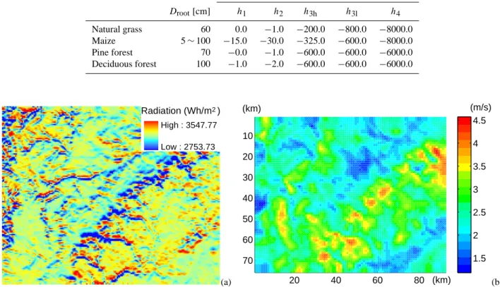
Fig. 4. Mean daily actual radiation (a) and wind pattern (b) in the study area.
stages. The critical pressure values for root water uptake and root zone depths can be found in Table 1. Other parameters, when not specified are assigned the default values suggested by SWAP.
5 Results
5.1 Spatial patterns of radiation and wind
Daily radiation and wind speed patterns are generated with the adapted r.sun and METRAS PC model respectively. Ta-ble 2 shows the correlation between the simulated patterns of radiation and wind with three primary topographic parame-ters, i.e. elevation (δ), slope (β) and aspect (γ), for the outer domain. To be mentioned, correlation of radiation with as-pect and slope are calculated to their functional values of sine and cosine respectively, given the known trignometrical rela-tionship between radiation and topography. The dependence of wind on topographic is rather complicated, therefore the correlation coefficients are derived based on the original val-ues. It shows that aspect has a remarkable impact on ra-diation, whereas the most significant topographic factor for wind speed is elevation, which can also be verified from the mean radiation and wind patterns (see Fig. 4). In general, the
Table 2. Correlation between radiation/wind patterns and
topo-graphic parameters for the outer domain (ρ¯ is the yearly average of correlation coefficients between daily patterns and topographic parameters, andσis the corresponding standard deviation.ρ˜is the correlation coefficients of mean daily pattern with topographic pa-rameters.)
topographic parameters
−cosγ sinβ δ
radiation
¯
ρ 0.621 −0.437 0.142 σ 0.170 0.245 0.127
˜
ρ 0.739 −0.262 0.176
γ β δ
wind
¯
ρ 0.066 0.012 0.302 σ 0.007 0.011 0.066
˜
ρ 0.127 0.057 0.594
0 10 20 30 40 50 60 70 80 90 100
J F A M J S O D
Relative radiation difference (%)
-10 40 90 140 190 240
Relative wind difference (%)
Actual radiation
Potential radiation wind
(a)
0 5 10 15 20 25 30 35
J F A M J S O D
R
e
la
ti
ve radi
ati
on di
fference (%
)
-10 40 90 140 190 240
R
e
la
ti
ve w
ind di
fference (%
)
Potential radiation Actual radiation Aggregation 500 Aggregation 100 wind
(b)
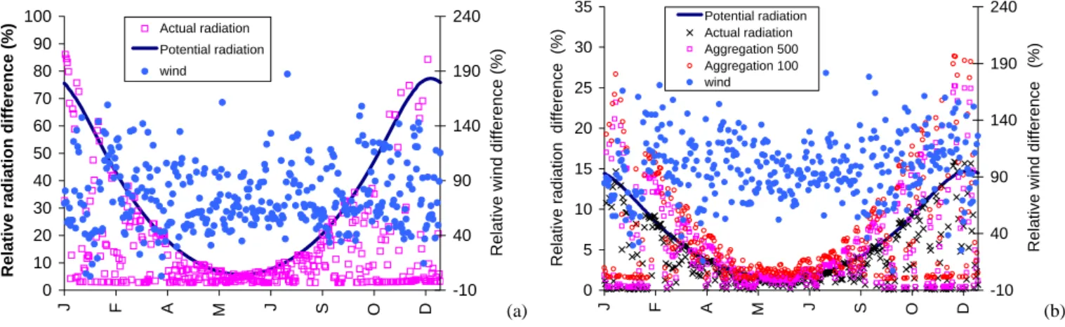
Fig. 5. Spatial variation of wind and radiation over time, (a) Inner domain and (b) outer domain.
Figure 5 shows the daily spatial variation of radiation and wind speed expressed in the interquantile range (NIQR),
P90−P10
µs , over the year. The spatial variabilities of both so-lar and wind are found to be very stable in summer but vary strongly in winter. The wind fields of both the in-ner and outer domain are simulated at 1000 m resolution. For both domains, the difference between the lower and up-per 10 quantile of wind force is around 80 % of the area mean wind speed, but can be as twice higher for some days (NIQR>2.0). For radiation, the inner domain is simulated at 100 m resolution whereas the outer domain is simulated at 1000 m resolution. In addition to actual radiation, the variability of potential radiation is also displayed in the fig-ure shown in the solid line, which is in general higher than the variability of actual radiation except for very few win-ter days. It is obvious that the NIQR is much higher at fine scale simulation (up to 90 %) than at the coarse scale (up to 15 %). To compare the loss of spatial variability of solar radiation at coarse scale, aggregated radiation from fine res-olution to coarse resres-olution is applied. Aggregations from both 100 m and 500 m to 1000 m have been tried. Given that the improvement by using 100 m is only marginal while the computational cost is 25 times more expensive, aggrega-tion from 500 m is applied in this study. Table 3 shows the mean daily spatial variation over the year and for two dif-ferent seasons, as well as the spatial variation of the mean daily radiation, both potential and actual, and of wind for both domains. Because finer resolution can better resolve the topographic diversity, it has caused stronger spatial vari-ability for the inner domain than the outer domain in terms of radiation. However, the wind pattern of the outer domain shows higher variability than the inner domain, because both domains are simulated at the same resolution and the outer domain covers more diversified topographic features. The potential radiation exhibits a much higher variation than the actual radiation, so does the variation in winter than in sum-mer. The seasonal variation of wind is more constant over the
Table 3. Spatial variability of wind and radiation (Summer gives the
average of daily NIQR from May to August, and winter averages daily NIQR from November to February. mean is the average of daily NIQR of the whole year, and yearly is the NIQR of mean daily wind or radiation of the year.)
Potential Actual wind radiation radiation
Inner domain
summer 8.96 % 5.8 % 73.2 % winter 57.5 % 26.9 % 82.0 % mean 32.8 % 14.1 % 75.8 % yearly 21.2 % 13.0 % 37.0 %
Outer domain
summer 2.1 % 2.0 % 95.7 % winter 11.2 % 8.2 % 100.9 % mean 6.7 % 5.3 % 97.9 % yearly 6.5 % 4.0 % 51.0 %
year with a slightly higher variation in winter than in sum-mer. For both radiation and wind, the mean daily NIQR is larger than the NIQR of the mean, which demonstrates the temporal dynamic of the spatial patterns.
5.2 Point results of SWAP
0 10 20 30 40 50 60
J F M A M J J A S O N D
[mm]
-15 -10 -5 0 5 10 15 20 25 30
[°C]
Precipitation Temperature
(a) 0 5 10 15 20 25 30 35
J F M A M J J A S O N D
[MJ/m
2]
0 2 4 6 8 10 12 14
[m/s]
P1 radiation P2 radiation p1 wind p2 wind
(b)
0 50 100 150 200 250 300 350
-150 -100 -50
Dept
h [cm]
0
Day number [-] (c)
0 50 100 150 200 250 300 350
-150 -100 -50 0
Depth [cm]
Day number [-]
0.3 0.32 0.34 0.36 0.38 0.4
(d)
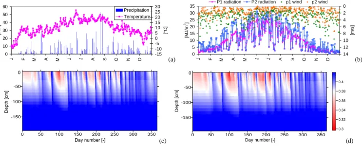
Fig. 6. Meteorological inputs and simulated soil moisture time series at P1 and P2. (a) Precipitation and temperature, (b) radiation and wind, (c) soil moisture profile at P1 and (d) soil moisture profile at P2.
and 6d show the soil moisture dynamics of the two points simulated at the spatial resolution of 100 m. The soil mois-ture dynamics of both points are similar, but P2 is obviously much drier than P1. The driest period is from 24 March to 11 April, during which there is no rainfall in around two weeks.
Table 4 shows the water balance at the two points sim-ulated with the two different soil configurations. At both scales, more water are evaporated/transpired at P2 associated correspondingly with a higher amount of total runoff gen-erated. There is only a minor difference between ETA and ETP, because southern Germany is a humid region, where ET is energy limited other than water availability limited pro-cess. The TA/TP ratio is higher than EA/EP, because water extraction capacity of root zone does not alter much under water stress conditions whereas the soil hydraulic conductiv-ity drops rapidly with decreasing saturation. EA is even more reduced with regard to EP for the more permeable soil con-figuration which have lower suction heads at the same degree of saturation. However, soil has very limited effects on the total amount of ET and runoff, it alters only the partition-ing between evaporation and transpiration, and between sur-face runoff and subsursur-face flow. Therefore, in case of more permeable soils, the declination of evaporation is offset by an enhanced transpiration, and meanwhile a stronger infiltra-tion causes consequently dominating drainage through sub-surface flow and negligible sub-surface runoff (1.0 mm).
As shown in the table, at 100 m resolution, the difference of potential and actual ET at the two points is around 20 %, while at 1000 m resolution the difference is reduced to 14 %. The difference of total runoff is 21 % at the fine scale and 15 % at the coarse scale. For less permeable soils, the dif-ference of surface runoff at the two scales are 12 % and 9 %
respectively. The results show that the variability in ET and runoff simulated at the two points diminishes with coarser resolution, but still at the coarser scale a significant spatial difference can be observed. Such strong heterogeneity in ET and runoff generation processes may lead to significant hy-drological consequences, such as local water balance or ero-sion patterns, etc.
5.3 Spatial results of SWAP
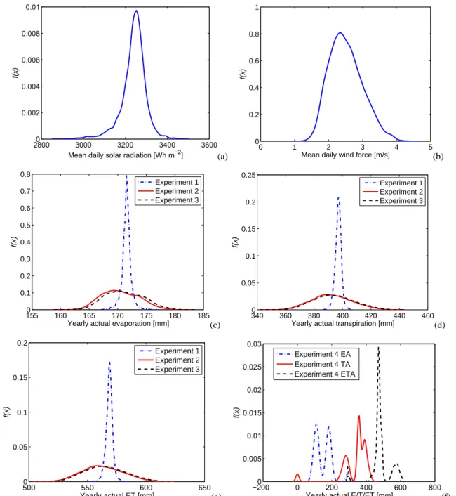
The spatial variabilities are also investigated at the two dif-ferent scales. Figure 7a and b show the statistical distribu-tions of spatial radiation and wind with the probability den-sity function (PDF) for the outer domain, and Fig. 7c–e show the PDFs of the yearly EA, TA, and ETA of the respective numerical experiments. The PDFs (EA, TA, ETA) of Exper-iment 1 which considers only radiation effects spread much narrower than the corresponding PDFs of other experiments. But the result of Experiment 2 is very close to Experiment 3, which reflects the domination of the wind effects over the radiation effects. The result of Experiment 4 show multiple peaks because of consideration of spatial land use. They are shown separately in Fig. 7f to avoid the distortion of other experiment results in the figure. To be mentioned, the nega-tive value in Fig. 7f is a numerical artifacts coming from the kernel smoothing of the distribution curve.
28000 3000 3200 3400 3600 0.002
0.004 0.006 0.008 0.01
Mean daily solar radiation [Wh m−2]
f(x)
(a)
0 1 2 3 4 5
0 0.2 0.4 0.6 0.8 1
Mean daily wind force [m/s]
f(x)
(b)
155 160 165 170 175 180 185 0
0.1 0.2 0.3 0.4 0.5 0.6 0.7 0.8
Yearly actual evaporation [mm]
f(x)
Experiment 1 Experiment 2 Experiment 3
(c)
3400 360 380 400 420 440 460 0.05
0.1 0.15 0.2 0.25
Yearly actual transpiration [mm]
f(x)
Experiment 1 Experiment 2 Experiment 3
(d)
5000 550 600 650
0.05 0.1 0.15 0.2
Yearly actual ET [mm]
f(x)
Experiment 1 Experiment 2 Experiment 3
(e)
−2000 0 200 400 600 800 0.005
0.01 0.015 0.02 0.025 0.03
Yearly actual E/T/ET [mm]
f(x)
Experiment 4 EA Experiment 4 TA Experiment 4 ETA
(f)
Fig. 7. Spatial variation of meteorological inputs and simulation results with SWAP for the of outer domain – (a) PDF of mean daily solar
radiation, (b) PDF of mean daily wind forece, (c) PDF of actual evaporation from Experiment 1, 2 and 3, (d) PDF of actual transpiration of Experiment 1, 2 and 3, (e) PDF of actual ET from Experiment 1, 2 and 3, (f) PDF of actual evaporation, actual transpiration and actual ET of Experiment 4.
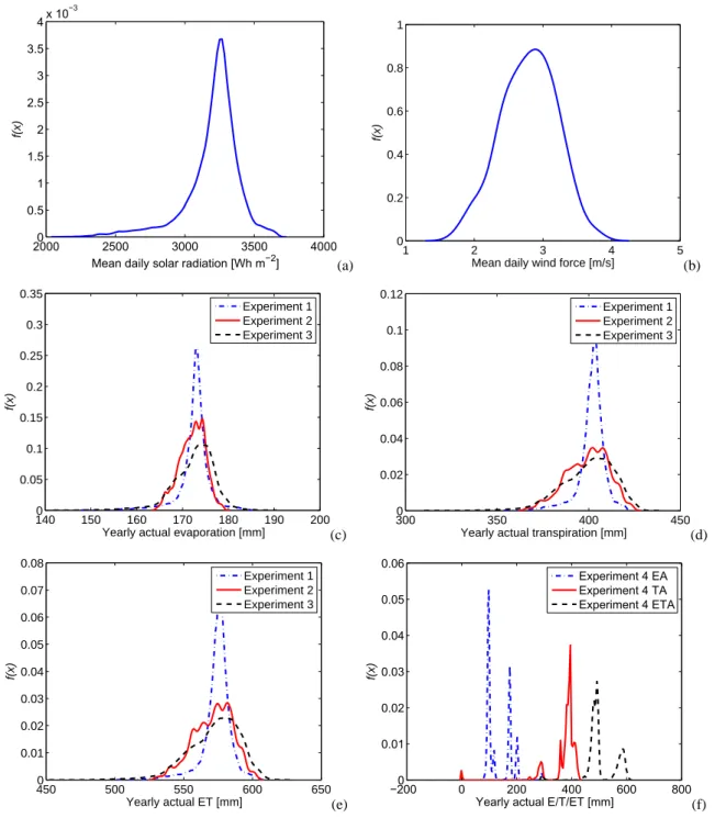
radiation aggregation from fine scale to coarse scale helps to maintain the spatial variation inherited from the fine scale, loss of spatial information and thus variation is unavoidable. Similarly to the outer domain, multiple peeks in the PDFs of EA, TA and ETA can be observed for the inner domain (see Fig. 8f). In general, agricultural field has the highest ET and ET is decreasing in the order of grass, deciduous forest, pine forest, to bare soil. Not only the amount of to-tal ET, but also the partitioning between evaporation (E) and
transpiration (T) changes with plant type, for example, forest shows higher transpiration because of the strong root uptake capability and higher vegetation cover of soil.
20000 2500 3000 3500 4000 0.5
1 1.5 2 2.5 3 3.5
4x 10
−3
Mean daily solar radiation [Wh m−2]
f(x)
(a)
1 2 3 4 5
0 0.2 0.4 0.6 0.8 1
Mean daily wind force [m/s]
f(x)
(b)
1400 150 160 170 180 190 200 0.05
0.1 0.15 0.2 0.25 0.3 0.35
Yearly actual evaporation [mm]
f(x)
Experiment 1 Experiment 2 Experiment 3
(c)
3000 350 400 450
0.02 0.04 0.06 0.08 0.1 0.12
Yearly actual transpiration [mm]
f(x)
Experiment 1 Experiment 2 Experiment 3
(d)
450 500 550 600 650
0 0.01 0.02 0.03 0.04 0.05 0.06 0.07 0.08
Yearly actual ET [mm]
f(x)
Experiment 1 Experiment 2 Experiment 3
(e)
−2000 0 200 400 600 800
0.01 0.02 0.03 0.04 0.05 0.06
Yearly actual E/T/ET [mm]
f(x)
Experiment 4 EA Experiment 4 TA Experiment 4 ETA
(f)
Fig. 8. Spatial variation of meteorological inputs and simulation results with SWAP for the inner domain – (a) PDF of mean daily solar
radiation, (b) PDF of mean daily wind forece, (c) PDF of actual evaporation from Experiment 1, 2 and 3, (d) PDF of actual transpiration of Experiment 1, 2 and 3, (e) PDF of actual ET from Experiment 1, 2 and 3, (f) PDF of actual evaporation, actual transpiration and actual ET of Experiment 4.
1.2 % variation in annual total ETA is resulted from 4.0 % variation of yearly radiation, with 8.0 % ETA variation from 51.0 % variation of yearly mean wind. For the inner domain, 13.0 % variation in radiation and 37.0% variation in wind are corresponding to 3.5 % and 6.4 % variation in ETA re-spectively. For both domains, the wind-caused spatial ETA
Table 4. Comparison of point simulation results for P1 and P2 under two different soil configurations.
P1 P2
100 m 1000 m 100 m 1000 m
elevation[m] 616 608 820 811
aspect[degree] 315.0 6.92 194.5 188.8
slope[degree] 26.98 5.74 5.97 1.46
mean radiation[MJ m−2] 9.33 10.54 12.25 11.98
mean wind[m s−1] 1.73 3.10
Acutal soil (Soil A & B)
Initial water storage[mm] 801.5 802.1 786.0 786.7 transpiration[mm] 339.1 (343.1) 357.1 (360.9) 417.1 (419.6) 414.1 (416.6) evaporation[mm] 154.3 (197.4) 161.9 (214.7) 177.7 (248.8) 176.1 (244.9)
drainage[mm] 509.7 486.7 411.5 416.3
runoff[mm] 88.0 85.9 78.7 78.9
Final water storage[mm] 816.8 817.1 807.4 807.8 Test soil (Soil C & D)
Initial water storage[mm] 654.2 656.1 601.2 603.6 transpiration[mm] 344.3 (344.3) 361.9 (361.9) 421.7 (421.7) 418.7 (416.6) evaporation[mm] 146.6 (196.2) 153.2 (213.6) 167.3 (246.7) 165.8 (244.9)
drainage[mm] 600.9 577.5 495.8 500.0
runoff[mm] 0.8 0.2 0.3 0.0
Final water storage[mm] 668.2 669.8 622.6 624.6
Note: The values in the parentheses are potential values.
Table 5. Annual results from the numerical experiments with SWAP for the outer domain.
Spatial variation P90−P10
µs of yearly total(%) Annual area mean (mm)
EA EP TA TP ETA ETP SMC∗ EA EP TA TP
EX 1 1.0 2.1 1.3 1.1 1.2 1.5 2.0 172.0 236.0 398.1 401.3 EX 2 4.9 6.2 9.3 9.0 8.0 8.0 2.4 170.9 233.9 393.5 396.7 EX 3 5.0 6.8 9.4 9.0 8.1 8.2 2.4 171.6 235.7 395.0 398.3 EX 4 62.2 113.7 39.7 33.5 24.6 34.7 4.4 150.6 228.9 336.1 359.9
∗Mean daily spatial soil moisture variation over the year.
than the ratio between wind and ET. In all cases, the spa-tial variation of the actual value is smaller than the poten-tial value for evaporation, while transpiration shows in most cases different behaviour, i.e. variation of potential transpira-tion is smaller than variatranspira-tion of actual transpiratranspira-tion. The rea-son may come from the threshold effects of root uptake under stress conditions as shown in Fig. 3 which may cause a spa-tially heterogeneous reduction of TA from TP, whereas the reduction of soil water transfer is more continuous. In this study, the actual E/T/ET at both scales happen to decrease from Experiment 1 to Experiment 3, which is related to the specific topography of the study area and should not be con-sidered as general. But the remarkable decrease of E/T/ET
when actual land use is considered is logical, because grass is one of the land uses with strongest ET.
Table 6. Annual results from the numerical experiments with SWAP for the inner domain.
Spatial variation P90−P10
µs (%) Annual area mean (mm)
EA EP TA TP ETA ETP SMC∗ EA EP TA TP
EX 1 3.6 7.0 3.5 3.4 3.5 4.7 1.8 173.1 237.4 402.8 405.8 EX 2 4.1 5.1 7.4 7.1 6.4 6.4 2.0 172.6 236.7 400.4 403.4 EX 3 6.1 9.3 9.1 8.7 8.1 8.8 2.2 172.9 237.3 400.7 403.7 EX 4 77.5 148.2 31.7 28.9 22.9 33.4 4.0 134.3 180.7 374.7 378.0
∗Mean daily spatial soil moisture variation over the year.
Table 7. Seasonal results of the numerical experiments for the outer domain.
Mean/maximum of daily spatial variationP90−P10 µs (%)
EA EP TA TP ETA ETP SMC
EX 1
winter 15.5 15.6 2.6 2.0 3.9 3.7 4.6
summer 0.8 1.5 1.9 1.0 1.5 1.2 1.7
mean 5.6 6.2 4.1 2.8 2.0 3.4 2.0
EX 2
winter 51.9 52.2 57.0 56.7 54.9 54.7 5.0
summer 5.4 7.9 12.4 11.7 8.8 8.5 2.1
mean 32.4 34.2 40.5 40.0 37.1 36.9 2.4
EX 3
winter 58.6 58.9 57.2 56.9 55.2 55.0 5.0
summer 7.8 8.4 12.6 11.9 9.0 8.7 2.2
mean 34.6 36.7 40.8 40.0 37.5 37.4 2.4
EX 4
winter 179.5 200.0 186.6 237.0 133.2 141.0 6.19 summer 101.4 136.9 107.0 48.6 74.0 64.6 4.4 mean 135.0 165.5 164.2 174.3 99.6 95.8 4.8
the varying interaction of radiation and wind over time. To have an insight of the spatial variation over time, the daily mean spatial variations from the outer domain are calculated for winter (from November to Feburary) and summer (from May to August) respectively in Table 7.
It is shown that for all 4 experiments, the variation of E/T/ET/SMC are stronger in winter than in summer. The seasonal difference in ET of Experiment 1 is mainly caused by radiation with little effect from the wind, as the resulting variation of ET is almost proportional to the variation of radi-ation for the two different seasons. However, in winter plant transpiration (NIQR = 2.6 and 2.0) is much less affected by radiation than soil evaporation (NIQR = 15.5 and 15.6), and the opposite holds for summer. This may have a strong im-plication for the spring flood in some regions. Experiment 2 shows that the effect of wind is conditioned differently on ra-diation for the two different seasons. In winter, wind is the major driving force for ET, the variation of wind is almost fully translated to the variation of the resulting ET. But in summer, radiation is dominating wind for the ET process, therefore strong spatial wind variation leads to only very
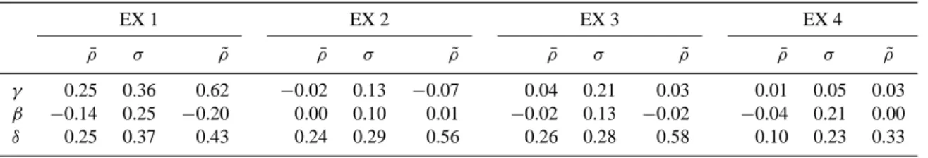
Table 8. Correlation between ET patterns and topographic parameters for the outer domain (ρ¯ is the yearly mean of daily correlation coefficients between daily ET pattern and topographic parameters, andσ is the corresponding standard deviation. ρ˜is the correlation of mean daily ET pattern with topographic parameters.)
EX 1 EX 2 EX 3 EX 4
¯
ρ σ ρ˜ ρ¯ σ ρ˜ ρ¯ σ ρ˜ ρ¯ σ ρ˜
γ 0.25 0.36 0.62 −0.02 0.13 −0.07 0.04 0.21 0.03 0.01 0.05 0.03 β −0.14 0.25 −0.20 0.00 0.10 0.01 −0.02 0.13 −0.02 −0.04 0.21 0.00 δ 0.25 0.37 0.43 0.24 0.29 0.56 0.26 0.28 0.58 0.10 0.23 0.33
strong with ρ˜ being 0.62 for aspect and 0.56 for elevation respectively. When the spatial heterogeneity of both radia-tion and wind are considered, the resulting ETA shows cor-relation only to elevation, which seems to confirm again the domination of wind over radiation. As shown in the results of Experiment 4, the dependence of ETA on elevation can still be detected (ρ¯= 0.10), even if spatial land use is consid-ered. Because of the assumption of linear groundwater table in this study, SMC will show predominantly correlation to elevation, which is trivial to be listed in the table.
To have a close look at the varying ET pattern over time, Fig. 9 shows the spatial variation of actual ET over the year for the outer domain resulted from Experiment 3 as an exam-ple. In the winter time, although the amount of ET is rela-tively small, the variation in terms of NIQR can be as high as 180 %, which may have an implication on spring and winter flood.
6 Discussion
In this paper, numerical experiments with the SWAP model have been applied to a mountainous region at two different scales to simulate ET and SMC and examine the effects of spatial radiation and wind induced by topography on them. The study applies physically-based models to simulate spa-tial radiation and wind, and analyzes the resulting spaspa-tial variation of ET/SMC. Simulations with spatial vegetation in-formation obtained from MODIS LAI are also performed to check the effect of land use on ET/SMC. The result shows that both radiation and wind vary strongly over spatial, with radiation being aspect dependent and wind being elevation dependent. The spatial variation of radiation is much higher in winter than in summer, while the spatial variation of wind is relatively constant over the year. Investigation at locations with distinct topographic features have shown that the differ-ence in incoming radiation and wind will lead to strong dif-ference in ET/SMC. The spatial difdif-ference in ET is offset by the amount of runoff generated, which may have an implica-tion in flood generaimplica-tion. Different soil condiimplica-tions will change the partitioning between evaporation and transpiration and, the partitioning between surface runoff and subsurface flow,
0 20 40 60 80 100 120 140 160 180
J J M A M M J J A S O N D
[%]
Fig. 9. Daily spatial variation of ETA from Experiment 3 for the
outer domain.
predominantly dependence on elevation under the interaction of radiation and wind, and such dependence can still be de-tected, even if spatial land use is considered.
In this study, the SWAP model is applied with radiation and wind data mapped from global data and physically-based model, which demand very few observation data. Because the lack of groundwater data, a linear groundwater table is assumed for the numerical experiments which may be im-proved by coupling the SWAP model with a groundwater model to update the groundwater level at each time step. However, the methodology applied in this research can still serves as a general approach for ETA simulation for data-sparse regions.
This study has confirmed the effects of topographic in-duced spatial radiation and wind on ET, and this informa-tion may be utilized to improve hydrological concepts in ET/SMC modeling. Moore et al. (1993) derived a dimen-sionless evaporation scaling ratio based on spatial radiation differences. Vertessy et al. (1990) developed a radiation weighted wetness index, which is a combination of potential solar radiation index (the ratio of the potential solar radiation on a sloping surface to that on a horizontal surface) and wet-ness index. As demonstrated in this study wind is in some cases dominating radiation, therefore the inclusion of wind effect into the wetness index following a statistical approach should be considered in the future.
Acknowledgements. The authors thank the International
Post-graduate Studies in Water Technologies (IPSWaT) of the German Federal Ministry of Education and Research (BMBF) and the International Doctoral Program Environment Water (ENWAT) at the University of Stuttgart for support of the research.
Edited by: I. Neuweiler
References
Andersen, J., Sandholt, I., Jensen, K. H., Refsgaard, J. C., and Gupta, H.: Perspectives in using a remotely sensed dryness index in distributed hydrological models at the river-basin scale, Hy-drol. Process., 2987, 2973–2987, doi:10.1002/hyp.1080, 2002. Baklanov, A., Fay, B., Kaminski, J., and Sokhi, R.: Overview of
Ex-isting Integrated (off-line and on-line) Mesoscale Meteorological and Chemical Transport Modelling Systems in Europe, WMO publications, Tech. rep., COST (Enhancing Mesoscale Meteo-rological Modelling Capacities for Air Pollution and Dispersion Applications) and GURME (GAW Urban Research Meteorology and Environment Project), 2008.
Bastiaanssen, W. G. M., Menenti, M., Feddes, R. A., and Holtslag, A. A. M.: A remote sensing surface energy balance algorithm for land (SEBAL), 1. Formulation, J. Hydrol., 212-213, 198–212, doi:10.1016/S0022-1694(98)00253-4, 1998.
Beven, K. J. and Kirkby, M. J.: A physically based , variable con-tributing area model of basin hydrology, Hydrolog. Sci. Bull., 24, 43–69, 1979.
Beven, K. J., Lamb, R., Quinn, P., Romanowicz, R., and Freer, J.: TOPMODEL, in: Computer models of watershed hydrol-ogy, edited by: Singh, V. P., Highlands Ranch, Colo., Water Re-sources Publications, 1995.
Black, T. A., Gardner, W. R., and Thurtell, G. W.: The prediction of evaporation, drainage and soil water storage for a bare soil, Soil Sci. Soc. Am., 33, 655–660, 1969.
Boesten, J. and Stroosnijder, L.: Simple model for daily evaporation from fallow tilled soil under spring conditions in a temperate cli-mate, Neth. J. Agr. Sci., 34, 75–90, 1986.
Bois, B., Pieri, P., Leeuwen, C. V., Wald, L., Huard, F., Gaudillere, J.-P., and Saur, E.: Using remotely sensed so-lar radiation data for reference evapotranspiration estimation at a daily time step, Agr. Forest Meteorol., 148, 619–630, doi:10.1016/j.agrformet.2007.11.005, 2008.
Bresnahan, P. A. and Miller, D. R.: Choice of data scale: predict-ing resolution error in a regional evapotranspiration model, Agr. Forest Meteorol., 84, 97–113, 1997.
Cano, D., Monget, J. M., Albuisson, M., Regas, H. G., and Wald, L.: A method for the determination of the global solar radiation from meteorological satellite data, Sol. Energy, 37, 31–39, 1986. Carlson, T. N., Capehart, W. J., and Gillies, R. R.: A new look at the simplified method for remote sensing of daily evapotranspi-ration, Remote Sens. Environ., 54, 161–167, doi:10.1016/0034-4257(95)00139-R, 1995.
Cassardo, C., Balsamo, G. P., Cacciamani, C., Cesari, D., Paccagnella, T., and Pelosini, R.: Impact of soil surface moisture initialization on rainfall in a limited area model: a case study of the 1995 South Ticino flash flood, Hydrol. Process., 16, 1301– 1317, 2002.
Cleugh, H. A., Leuning, R., Mu, Q., and Running, S. W.: Regional evaporation estimates from flux tower and MODIS satellite data, Remote Sens. Environ., 106, 285–304, 2007.
Crave, A.: The influence of topography on time and space distribu-tion of soil surface water content, Hydrol. Process., 11, 203–210, 1997.
Dingman, S. L.: Physical Hydrology, Prentice-Hall, Inc., 2nd Edn., 2002.
El Maayar, M. and Chen, J. M.: Spatial scaling of evapotran-spiration as affected by heterogeneities in vegetation, topog-raphy, and soil texture, Remote Sens. Environ., 102, 33–51, doi:10.1016/j.rse.2006.01.017, 2006.
FAO: Expert consultation on revision of FAO methodologies for crop water requirements, ANNEX V: FAO Penman-Monteith Formula, Tech. rep., FAO, Rome, Italy, 1990.
Florinsky, I., Eilers, R., Manning, G., and Fuller, L.: Prediction of soil properties by digital terrain modelling, Environ. Model. Softw., 17, 295–311, doi:10.1016/S1364-8152(01)00067-6, 2002.
Frank, H. and Landberg, L.: Modelling waving crops in a wind tunnel, Bound.-Lay. Meteorol., 85, 359–377, 1997.
Hofierka, J. and Suri, M.: The solar radiation model for Open source GIS: implementation and application, in: Proceddings of the Open source GIS – GRASS users conference 2002, Trento, Italy, 2002.
Jensen, M., Burman, R., and Allen, R.: Evapotranspiration and irri-gation water requirements, ASCE manuals and reports on engi-neering practice 70, ASCE, New York, 1990.
Kalnay, E., Kanamitsu, M., Kistler, R., Collins, W., Deaven, D., Gandin, L., Iredell, M., Saha, S., White, G., Woollen, J., Zhu, Y., Leetmaa, A., Reynolds, R., Chelliah, M., Ebisuzaki, W., Hig-gins, W., Janowiak, J., Mo, K. C., Ropelewski, C., Wang, J., Jenne, R., and Joseph, D.: The NCEP/NCAR 40-year reanalysis project, B. Am. Meteorol. Soc., 77, 437–471, doi:10.1175/1520-0477(1996)077<0437:TNYRP>2.0.CO;2, 1996.
Kasten, F.: Parametriserung der Globalstrahlung durch Bedeck-ungsgrad und Trbungsfaktor, Ann. Meteorol., 20, 49–50, 1983. Lenz, C. J., M¨uller, F., and Schl¨unzen, K.: The sensitivity of
mesoscale chemistry transport model results to boundary values, Environ. Monitor. Assess., 65, 287–295, 2000.
Liu, M., B´ardossy, A., Li, J., and Jiang, Y.: GIS-based modeling of topography-induced solar radiation variability in complex terrain for data sparse region, Int. J. Geogr. Inf. Sci., in press, 2011. Mikhail Sofiev, A. I. and Miranda, R. S.: Joint report of COST
Ac-tion 728 and GURME: Review of the capacities of meteorolog-ical and chemistry-transport models for describing and preidict-ing air pollution episodes, WMO publications, Tech. rep., COST – Enhancing Mesoscale Meteorological Modelling Capacities for Air Pollution and Dispersion Applications – and GURME – GAW Urban Research Meteorology and Environment Project, 2009.
Mohanty, B. P. and Skaggs, T. H.: Spatio-temporal evolution and time-stable characteristics of soil moisture within remote sensing footprints with varying soil, slope, and vegetation, Adv. Water Resour., 24, 1051–1067, doi:10.1016/S0309-1708(01)00034-3, 2001.
Moore, I. D., Gallant, J. C., and Guerra, L.: Modelling the spa-tial variability of hydrological process using GIS, in: Hydro-GIS 93: Application of Geographic Information System in Hy-drology and Water Resources, Proceedings of Viena Conference, IAHS Publication, 1993.
Mu, Q., Heinsch, F. A., Zhao, M., and Running, S. W.: Develop-ment of a global evapotranspiration algorithm based on MODIS and global meteorology data, Remote Sens. Environ., 111, 519– 536, doi:10.1016/j.rse.2007.04.015, 2007.
Norbiato, D., Borga, M., Esposti, S. D., Gaume, E., and Anquetin, S.: Flash flood warning based on rainfall thresholds and soil moisture conditions: An assessment for gauged and ungauged basins, J. Hydrol., 362, 274–290, 2008.
Odeh, I. O. A., McBratney, A. B., and Chittleborough, D. J.: Spa-tial prediction of soil properties from landform attributes derived from a digital elevation model, Geoderma, 63, 197–214, 1994. Ostendorf, B. and Reynolds, J. F.: A model of arctic tundra
veg-etation derived from topographic gradients, Landscape Ecology, 187–201, 1998.
Penman, H. L.: Natural evaporation from open water, bare soil and grass, P. Roy. Soc. A, 193, 120–146, 1948.
Price, J.: Using Spatial Context in Satellite Data to Infer Regional Scale Evapotranspiration, IEEE T. Geosci. Remote, 28, 940–948, 1990.
Quinn, P. F. and Beven, K. J.: Spatial and temporal predictions of soil moisture dynacmics, runoff, variable source areas and evap-otranspiration for plynlimon, Mid-Wales, Source, 7, 425–448, 1993.
Reed, D. N., Anderson, T. M., Dempewolf, J., Metzger, K., and Serneels, S.: The spatial distribution of vegetation types in the Serengeti ecosystem: the influence of rainfall and topographic relief on vegetation patch characteristics, J. Biogeogr., 36, 770– 782, doi:10.1111/j.1365-2699.2008.02017.x, 2009.
Rigollier, C., Lef`evre, M., and Wald, L.: The method Heliosat-2 for deriving shortwave solar radiation from satellite images, Sol. Energy, 77, 159–169, 2004.
Schl¨unzen, K. H., Bigalke, K., L¨upkes, C., and Panskus, H.: Doc-umentation of the mesoscale transport- and fluid model ME-TRAS PC as part of model system MEME-TRAS+, Tech. rep., Me-teorologisches Institut, Universitt Hamburg, mETRAS Technical Rep. 11, 2001.
Schr¨oder, B.: Pattern, process, and function in landscape ecology and catchment hydrology – how can quantitative landscape ecol-ogy support predictions in ungauged basins?, Hydrol. Earth Syst. Sci., 10, 967–979, doi:10.5194/hess-10-967-2006, 2006. Schueler, S. and Schl¨unzen, K. H.: Modeling of oak pollen
disper-sal on the landscape level with a mesoscale atmospheric model, Environ. Model. Assess., 11-3, 179–194, 2006.
Su, Z.: The Surface Energy Balance System (SEBS) for estima-tion of turbulent heat fluxes, Hydrol. Earth Syst. Sci., 6, 85–100, doi:10.5194/hess-6-85-2002, 2002.
Thornthwaite, C. W. and Mather, J. R.: The Water Balance, Publ. Climatol., 8, 188, 1955.
Thornton, P. E., Running, S. W., and White, M. A.: Generating surfaces of daily meteorological variables over large regions of complex terrain, J. Hydrol., 190, 214–251, doi:10.1016/S0022-1694(96)03128-9, 1997.
van Dam, J., Huygen, J., Wesseling, J. R. A. F., Kabat, P., van Wal-sum, P., Groenendijk, P., and van Diepen, C.: Theory of SWAP version 2.0, Tech. rep., Department of Water Resources, Wa-geningen Agricultural University, WaWa-geningen, The Netherlands, 1997.
Guideline VDI 3783: Environmental Meteorology, Association of German Engineers, 2005.
Verstraeten, W. W., Veroustraete, F., and Feyen, J.: Assessment of Evapotranspiration and Soil Moisture Content Across Different Scales of Observation, Sensors, 8, 70–117, 2008.
Vertessy, R., Wilson, C., Silburn, D., Connolly, R., and Ciesiolka, C.: Predicting erosion hazard areas using digital terrain analysis, AHS AISH Publ., 192, 298–308, 1990.
Wang, K., Wang, P., Li, Z., Cribb, M., and Sparrow, M.: A simple method to estimate actual evapotranspiration from a combination of net radiation , vegetation index , and temperature, J. Geophys. Res., 112, 1–14, doi:10.1029/2006JD008351, 2007.
Western, A. W., Grayson, R. B., Bl¨oschl, G., and Willgoose, G. R.: Observed spatial organization of soil moisture indices, Water Re-sour., 35, 797–810, 1999.
Western, A. W., Grayson, R. B., and Bl¨oschl, G.: Scaling of Soil Moisture: A Hydrologic Perspective, Ann. Rev. Earth Planet. Sc., 30, 149–180, 2002.
Wu, Z. and Schl¨unzen, K. H.: Numerical study on the local wind structures forced by the complex terrain of Qingdao area, Acta Meteorol. Sinica, 6, 355–366, 1992.
Yang, W., Tan, B., Huang, D., Rautiainen, M., Shabanov, N. V., Wang, Y., Privette, J. L., Huemmrich, K. F., Fensholt, R., Sand-holt, I., Weiss, M., Ahl, D. E., Gower, S. T., Nemani, R. R., Knyazikhin, Y., and Myneni, R. B.: MODIS Leaf Area Index Products: From Validation to Algorithm Improvement, IEEE T. Geosci. Remote, 44, 1885–1898, 2006.