TD-88Up – UPGRADED NEUTRAL EARTH’S
THERMOSPHERE TOTAL DENSITY TD-88 MODEL
B. ˇSurlan1
and S. ˇSegan2 1
Mathematical Institute of the Serbian Academy of Sciences and Arts, Kneza Mihaila 36, 11001 Belgrade, Serbia
E–mail: [email protected]
2
Department of Astronomy, Faculty of Mathematics, University of Belgrade Studentski trg 16, 11001 Belgrade, Serbia
E–mail: [email protected]
(Received: January 6, 2009; Accepted: March 7, 2009)
SUMMARY: Improved constants of the total density TD-88 model for the Earth’s neutral thermosphere are calculated. The model is fully functional within the height range of 200 to 500 km, with fixed values of the mean solar flux and geomagnetic index. The control data of the atmospheric air density are derived from the aero-nomical NRLMSISE-00 model which was used as the reference one. The upgraded TD-88, named TD-88Up, model is obtained by the extended LSQ method with varying all model parameters.
Key words. Earth
1. INTRODUCTION
Since the times when the first artificial satel-lite was launched, it was realized that the changes of orbital elements of the Low Earth Orbit (LEO) satellite are connected with variations in the upper atmosphere. These changes are caused by the atmo-spheric drag and this perturbing force has become a very powerful tool for studying the upper layers of planetary atmospheres.
By numerical integration of the equations of the satellite perturbed motion or by analytical meth-ods, the total density of the atmosphere around the satellite’s path can be obtained. On the other hand, to predict orbits of LEO satellites with the satisfac-tory accuracy, it is necessary to know the distribution and variation of the atmospheric density which can be obtained from an assumed atmospheric model.
The most commonly used models are the aero-nomical ones, which are very precise and effective for certain purposes, but in the theory of satellite motion many difficulties in their application appear. Because of this, a better way is to define an analyt-ical or semi-analytanalyt-ical model of atmospheric density distribution. This enables an analytical treatment of the perturbations of the satellite orbital elements and, using the reverse procedure, to obtain the model parameters, too.
Such a model is the Total Density (TD) model of the Earth’s neutral thermosphere, and some vari-ants of it (Sehnal 1988, Sehnal and Posp´ıˇsilov´a 1988, Bezdˇek and Vokrouhlick´y 2004).
aero-nomical models. In our previous paper (ˇSegan and ˇ
Surlan 2005) we showed how to improve the TD-88 model using the up-to-date aeronomical NRLMSISE-00 model (Picone et al. 2NRLMSISE-002). An improved agree-ment among these models was achieved by fitting their differences in the case with only two variable model parameters. However, an even better agree-ment is achieved by varying all the parameters si-multaneously.
2. THE ATMOSPHERIC DENSITY MODELS
The TD-88 model (Sehnal and Posp´ıˇsilov´a
1988) is an improved TD model (Sehnal 1988). The air density (ρ) is described by the expression
ρ=fxf0k0 7
X
n=1
hngn , (1)
where
fx= 1 +a1(Fx−Fb),
f0=a2+fm,
fm= (Fb−60)/160,
k0= 1 +a3(Kp−3).
To include the solar and geomagnetic effects and, moreover, the individual terms containing factors de-pendent on the mean solar flux, the coefficients gn
are used. Through these coefficients the average den-sity, the individual mean solar flux dependence, the north-south asymmetry, annual and semi-annual, di-urnal and semi-didi-urnal variations are included. The altitude dependence is described by thehn terms,
hn =Kn,0+ 3
X
j=1
Kn,jexp
Ã
120−h
29j !
, (2)
and the functionsgn are given by
g1= 1
g2=fm/2 +a4
g3= sin (d−p3) sinϕ
g4= (a5fm+ 1) sin (d−p4)
g5= (a6fm+ 1) sin 2(d−p5)
g6= (a7fm+ 1) sin (t−p6) cosϕ
g7= (a8fm+ 1) sin 2(t−p7) cos 2
ϕ.
The symbols denote: Kn,j,ai – numerical constants
of a model, pn – phases, Fx – solar flux measured
at 10.7 cm for previous day, Fb – mean solar flux
averaged over three solar rotations, Kp –
geomag-netic index 3 hours before the current local time, h – altitude,ϕ– latitude, andt – local time.
On the other side, the NRLMSISE-00 model is an empirical model of the Earth’s neutral atmosphere valid from the ground up to the height of 1000 km of altitude. The densities for a given day in a year (IYD), the universal time in seconds (SEC), the alti-tude (ALT), latialti-tude (GLAT), longialti-tude (GLONG),
local time (STL), the mean solar flux averaged over three solar rotations (F107A), the solar flux mea-sured at 10.7 cm for previous day (F107) and the geomagnetic index (Ap) can be found at the Naval Research Laboratory web site.1
3. THE UPGRADING PROCEDURE
Till now, several improvements of the Sehnal’s basic TD model have been made (Sehnal and Posp´ıˇsilov´a 1988, Bezdˇek and Vokrouhlick´y 2004).
In this work, we first determined the Kn,j model
constants. The parametersai andpn are considered
as known, and for them we use the same values as in the TD-88 model. The procedure consisted of the following steps:
(i) Linearizing the density expression (1) with re-spect toKn,j.
(ii) Varying all the parameters simultaneously.
(iii) Determining the new Kn,j constants of the
model, and their standard deviations (within an altitude range from 200 to 500 km). (iv) Estimating accuracy of the obtained model
constants.
(v) Comparing with the NRLMSISE-00 model.
We choose the longitude value GLONG=0◦as
a reference one; the variation of density with longi-tude was not considered, because this type of varia-tion was not included in the TD-88 model. The uni-versal time is expressed in seconds (SEC=STL·3600). The solar flux for the previous day is calculated from
F107 = (1.+ 0.15N)F107A, N=−1,0,1. (3)
We have used theKpindex rather than theApindex
as the parameter of geomagnetic activity.
The boundary values of intervals of physical and geometrical parameters and their steps and num-ber of values are presented at Table 1. This led us to explore 221760 different density values as input data in our attempt to upgrade TD-88 model.
By extending the ordinary least square method (LSQ) and applying the linearization of the density expression (1) we computed the coefficients and their deviations for the upgraded model from
σ2 n,j=
Dii
D σ
2
0 , n= 1,7, j= 1,4, i= 1,28, (4)
whereDis the determinant of the matrix of the
sys-tem, Dii are algebraic complements of the diagonal
elements iiandσ2
0 is the standard deviation
σ2 0=
1 N−p
N
X
k=1
εk , N = 5460, p= 28, (5)
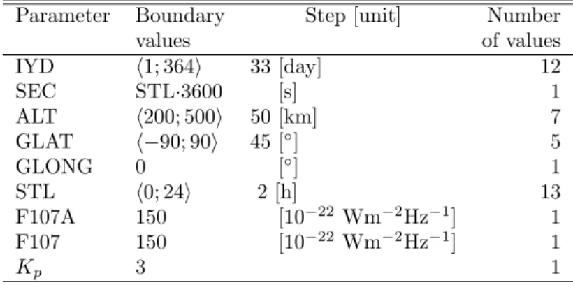
Table 1. The boundary values of intervals of physical and geometrical parameters, their steps and number of values for the first iteration.
Parameter Boundary Step [unit] Number
values of values
IYD h1; 331i 33 [day] 11
SEC STL·3600 [s] 1
ALT h200; 500i 50 [km] 7
GLAT h−80; 80i 40 [◦] 5
GLONG 0 [◦] 1
STL h1; 22i 3 [h] 8
F107A h60; 260i 40 [10−22
Wm−2
Hz−1
] 6
F107 Eqn. (3) [10−22
Wm−2
Hz−1
] 3
Kp h0; 9i 3 4
Table 2. The boundary values of intervals of physical and geometrical parameters, their steps and number of values which give the most accurate results.
Parameter Boundary Step [unit] Number
values of values
IYD h1; 364i 33 [day] 12
SEC STL·3600 [s] 1
ALT h200; 500i 50 [km] 7
GLAT h−90; 90i 45 [◦] 5
GLONG 0 [◦] 1
STL h0; 24i 2 [h] 13
F107A 150 [10−22
Wm−2
Hz−1
] 1
F107 150 [10−22
Wm−2
Hz−1
] 1
Kp 3 1
whereεk are the residuals obtained by changing the
calculated values ofKn,jin the conditional equation,
N is the total number of data, andpis the number
of unknown parameters. All calculations are made by FORTRAN90 routines.
4. RESULTS
In the first solution of the system of normal equations and densities calculation with the new set of constants, a small number of densities (about 1%) was negative. We checked the numerical correctness of the algorithms used and all matrix transforma-tions. Statistically, the results with negative densi-ties were with smaller scattering, but we had to find the cause for these nonrealistic values.
As a next step, we therefore analysed varia-tions of the parameters, and we found that variavaria-tions of the geomagnetic index and solar flux are those that give rise to nonrealistic densities. Further analysis of these variations and conditional equations of LSQ confirmed that for any combination of the geomag-netic index and solar flux we can determine set of Kn,j constants which give realistic densities.
Using the procedure of upgrading described above and exact values of the average solar flux and geomagnetic index obtained from measurements (or model) we can determine the constantsKn,j. Our set
of constants yields densities which agree better with the NRLMSISE-00 model than those of the TD-88 model.
By an additional analysis of the resulting den-sities, obtained by changing values of the geomag-netic index and solar flux, we concluded that the
most accurate results are obtained for Fx = Fb =
150, Kp = 3 (Ap = 15) and varying the other four
parameters (Table 2). In this section we present the set of constant which we determined for this case.
With these values of parameters we have de-rived density values of the upgraded TD-88 model.
The constants Kn,j and their error estimates are
shown in Tables 3 and 4. In this way we succeeded to upgrade the TD-88 model within the height range from 200 to 500 km. The upgrade of model we named the TD-88Up model.
5. COMPARISON OF THE NRLMSISE-00, TD-88, AND TD-88Up MODELS
In order to estimate the accuracy of the TD-88Up model we compared this model with the NRLMSISE-00 and the TD-88 models. The rela-tive (percentage) deviation (δ) forN = 5460 selected points with a combination of parameters given in
Ta-ble 2 is used to obtain total δ for the model. The
Table 3. ConstantsKn,j for the TD-88Up model.
n/j 0 1 2 3
1 0.133266·10−08
0.167935·10−07
0.678445·10−08
−0.558459·10−08
2 −0.405992·10−08
−0.400823·10−07
−0.195238·10−07
0.171885·10−07
3 −0.199071·10−13
−0.439091·10−09
−0.374988·10−10
−0.116933·10−10
4 0.407227·10−14
−0.250279·10−10
−0.434513·10−11
−0.151686·10−11
5 0.147905·10−13 −0.595860·10−10 −0.666754·10−11 −0.275309·10−11
6 −0.578693·10−14 −0.164250·10−09 0.521976·10−10 0.383611·10−10
7 0.117458·10−13 −0.185037·10−10 0.665665·10−11 −0.207915·10−12
Table 4. Standard deviationσ2
n,j of constantsKn,j for the TD-88Up model.
n/j 0 1 2 3
1 −0.47242·10−18
−0.14135·10−15
−0.17066·10−15
0.56410·10−17
2 −0.43818·10−17
−0.13113·10−14
−0.15828·10−14
0.52321·10−16
3 0.28125·10−24
0.84428·10−20
0.36202·10−20
0.63290·10−21
4 0.70778·10−26
0.21247·10−21
0.91104·10−22
0.15927·10−22
5 0.72667·10−26
0.21814·10−21
0.93534·10−22
0.16352·10−22
6 0.31438·10−24 0.94372·10−20 0.40466·10−20 0.70744·10−21
7 0.66498·10−26 0.19962·10−21 0.85595·10−22 0.14964·10−22
δ= 1 N
N
X
k=1
δk =
1 N
N
X
k=1
100|ρ1k−ρ2k| ρ2k
, (6)
whereρ1k are the densities obtained from either the
TD-88Up model or the TD-88,ρ2k are the densities
obtained from the NRLMSISE-00 model, and N is
the total number of data.
The standard deviation (σ) of the TD-88Up
model is given by
σ= 1 N
N
X
k=1
σk=
1 N
N
X
k=1
p
(ρ1k−ρ2k)2 . (7)
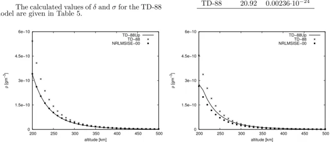
The calculated values ofδandσfor the TD-88 model are given in Table 5.
As it can be seen, with the newKn,jconstants
we attained a significantly better accuracy and a bet-ter agreement with the inbet-ternational standards. By the analysing the sigma values of the the TD-88Up model we concluded that the model agrees better with the NRLMSISE-00 model for altitudes 200–400 km and the largest differences between models ap-pear for altitudes 400–500 km.
Table 5. Relative and standard deviation of the TD-88Up and the TD-88 models with respect to the NRLMSISE-00 model.
Model δ[%] σ2
TD-88Up 7.14 0.00356·10−26
TD-88 20.92 0.00236·10−24
0 1.5e−10 3e−10 4.5e−10 6e−10
200 250 300 350 400 450 500
ρ
[gm
−3
]
altitude [km]
TD−88Up TD−88 NRLMSISE−00
0 1.5e−10 3e−10 4.5e−10 6e−10
200 250 300 350 400 450 500
ρ
[gm
−3
]
altitude [km]
TD−88Up TD−88 NRLMSISE−00
Fig. 1. Total density dependence on the altitude for the models TD-88Up , TD-88, and NRLMSISE-00 for
0 2e−11 4e−11 6e−11
−90 −45 0 45 90
ρ
[gm
−3
]
latitude [0]
TD−88Up TD−88 NRLMSISE−00
0 2e−12 4e−12 6e−12 8e−12
−90 −45 0 45 90
ρ
[gm
−3
]
latitude [0]
TD−88Up TD−88 NRLMSISE−00
Fig. 2. Latitudinal dependence of the total density for the models TD-88Up, TD-88, and NRLMSISE-00 forϕ∈ h−90; 90i,Fx=Fb= 150;Kp= 3; (Left)d= 80,t= 14,h= 300; (Right)d= 330,t= 18,h= 400.
200 250
300 350
400 450
500 10
-12 10
-11 10
-10
-90 -45
0 45
90
transparent grid - TD-88Up gray grid - NRLMSISE-00
altitude [km]
latitude [ 0 ] [gm
-3 ]
200 250
300 350
400 450
500 10
-12 10
-11 10
-10
-90 -45
0 45
90
transparent grid - TD-88Up gray grid - NRLMSISE-00
altitude [km]
latitude [ 0 ] [gm
-3 ]
Fig. 3. Total density dependence on the altitude and latitude for the TD-88Up (transparent grid) and NRLMSISE-00 (gray grid) models forϕ∈ h−90; 90i,h∈ h200; 500i,Fx=Fb = 150,Kp= 3; (Left)d= 80,
t= 14; (Right)d= 330,t= 18.
0 2e−11 4e−11 6e−11
0 4 8 12 16 20 24
ρ
[gm
−3]
local time [h]
TD−88Up TD−88 NRLMSISE−00
0 2e−12 4e−12 6e−12 8e−12 1e−11
0 4 8 12 16 20 24
ρ
[gm
−3]
local time [h]
TD−88Up TD−88 NRLMSISE−00
Fig. 4. Local time dependence of the total density for TD-88Up, TD-88, and NRLMSISE-00 models for
200 250
300 350
400 450
500 10
-12 10
-11 10
-10
0 4
8 12
16 20
24
altitude [km] local time [h]
[gm -3
]
transparent grid - TD-88Up gray grid - NRLMSISE-00
200 250
300 350
400 450
500 10
-12 10
-11 10
-10
0 4
8 12
16 20
24
transparent grid - TD-88Up gray grid - NRLMSISE-00
altitude [km] local time [h]
[gm -3
]
Fig. 5. Total density dependence on the altitude and on the local time as evaluated on the basis of the TD-88Up (transparent grid) and NRLMSISE-00 (gray grid) models fort∈ h0; 24i,h∈ h200; 500i,Fx=Fb= 150,
Kp= 3; (Left) d= 80,ϕ= 0; (Right)d= 330,ϕ= 90.
0 2e−11 4e−11 6e−11
0 60 120 180 240 300 360
ρ
[gm
−3
]
day of year
TD−88Up TD−88 NRLMSISE−00
0 2e−12 4e−12 6e−12 8e−12
0 60 120 180 240 300 360
ρ
[gm
−3
]
day of year
TD−88Up TD−88 NRLMSISE−00
Fig. 6. Seasonal (day of year) dependence of total density obtained from the TD-88Up, TD-88, and NRLMSISE-00 models for d∈ h0; 360i, Fx =Fb = 150, Kp = 3; (Left) t = 14, ϕ = 0, h= 300; (Right)
t= 18,ϕ= 90,h= 400.
200 250
300 350
400 450
500 10
-11 10
-10
0 60
120 180
240 300
360 transparent grid - TD-88Up gray grid - NRLMSISE-00
altitude [km]
day of year [gm
-3 ]
200 250
300 350
400 450
500 10
-12 10
-11 10
-10
0 60
120 180
240 300
360 transparent grid - TD-88Up gray grid - NRLMSISE-00
altitude [km]
day of year [gm
-3 ]
Fig. 7. Depedence of the total density on the altitude and on the day of year obtained by the TD-88Up (transparent grid) and NRLMSISE-00 (gray grid) models for d∈ h0; 360i,h∈ h200; 500i,Fx =Fb = 150,
Since the NRLMSISE-00 model is very precise and includes many short-term density variations (see Figs. 2 and 4) which were not present in the previ-ous empirical models, for example in the DTM model (Barlier et al. 1977) which was used for deriving constants of the TD-88 model, a good fitting of the TD-88 model to this model is a difficult task. Better agreement with the NRLMSISE-00 model could be obtained by correcting the analytical expression for the density (1), which is, however, beyond the scope of this paper.
Figs. 1 to 7 represent selected cases of models comparison. It can be seen from these figures that the agreement between models is not the same for any values of parameters.
Figs. 3, 6, and 7 display comparison of height density variations of TD-88Up and NRLMSISE-00 for varying latitude, local time, and day of the year. Regions where the models agree well and, conse-quently, where the plotted grids overlap, can be seen as ”lighter” ones, whereas regions with some dis-agreement appear ”darker”.
In Fig. 2 one can see that densities obtained from the NRLMSISE-00 model show variations with latitude, which are not very well described by the
TD- 88Up model. Also, in Fig. 4 densities
ob-tained from the NRLMSISE-00 model show varia-tions with local time, not only semi-diurnal but also terr-diurnal variations. For better agreement, these variations with latitude shoud be better analyticaly described in the TD-88Up model and terr-diurnal variations should be included.
6. CONCLUSIONS
The TD-88Up model gives better agreement with up-to-date data (the NRLMSISE-00 model) than the original TD-88 model. More comprehensive model can be achieved by increasing the number of terms in density expression, especially diurnal and terr-diurnal (diurnal-part) terms.
It is also possible to make some additional cor-rections of density variations by analyzing data re-garding the atmospheric drag and in situ data from satellites.
Acknowledgements– The authors are grateful to Dr Slobodan Ninkovi´c for careful checking of English in the manuscript and to an anonymous referee for his valuable comments.
REFERENCES
Barlier, F., Berger, C., Falin, J. L., Kockarts, G., Thullier, G.: 1977,Ann. Geophys.,34, 1. Bezdˇek, A., Vokrouhlick´y, D.: 2004, Planet. Space
Sci., 52, 1233.
Picone, J. M., Hedin, A. E., Drop, D. P., Aikin, A. C.: 2002,J. Geophys. Res. A,107, 1468.
Sehnal, L.: 1988, Bull. Astron. Inst. Czech., 39,
120.
Sehnal, L., Posp´ıˇsilov´a, L. : 1988, Preprint No. 67 of the Astron. Inst. Czech. Acad. Sci.
ˇ
Segan, S., ˇSurlan, B.: 2005, Serb. Astron. J., 171, 43.
TD–88Up – UNAPREENI MODEL TOTALNE
GUSTINE NEUTRALNE TERMOSFERE ZEMLjE
B. ˇSurlan1
and S. ˇSegan2 1
Mathematical Institute of the Serbian Academy of Sciences and Arts, Kneza Mihaila 36, 11001 Belgrade, Serbia
E–mail: [email protected]
2
Department of Astronomy, Faculty of Mathematics, University of Belgrade Studentski trg 16, 11001 Belgrade, Serbia
E–mail: [email protected]
UDK 523.31–852 Originalni nauqni rad
Uraena je popravka koeficijenata
TD-88 modela neutralne termosfere Zemlje.
Model je potpuno funkcionalan u opsegu
visina od 200 do 500 km, sa fiksnim
vred-nostima srednjeg solarnog fluksa i
geomag-netnog indeksa. Kontrolni podaci